Automatic Modeling of Opaque Code for JavaScript Static Analysis

Abstract

Static program analysis often encounters problems in analyzing library code. Most real-world programs use library functions intensively, and library functions are usually written in different languages. For example, static analysis of JavaScript programs requires analysis of the standard built-in library implemented in host environments. A common approach to analyze such opaque code is for analysis developers to build models that provide the semantics of the code. Models can be built either manually, which is time consuming and error prone, or automatically, which may limit application to different languages or analyzers. In this paper, we present a novel mechanism to support automatic modeling of opaque code, which is applicable to various languages and analyzers. For a given static analysis, our approach automatically computes analysis results of opaque code via dynamic testing during static analysis. By using testing techniques, the mechanism does not guarantee sound over-approximation of program behaviors in general. However, it is fully automatic, is scalable in terms of the size of opaque code, and provides more precise results than conventional over-approximation approaches. Our evaluation shows that although not all functionalities in opaque code can (or should) be modeled automatically using our technique, a large number of JavaScript built-in functions are approximated soundly yet more precisely than existing manual models.

1 Introduction

Static analysis is widely used to optimize programs and to find bugs in them, but it often faces difficulties in analyzing library code. Since most real-world programs use various libraries usually written in different programming languages, analysis developers should provide analysis results for libraries as well. For example, static analysis of JavaScript apps involves analysis of the builtin functions implemented in host environments like the V8 runtime system written in C++.

A conventional approach to analyze such opaque code is for analysis developers to create models that provide the analysis results of the opaque code. Models approximate the behaviors of opaque code, they are often tightly integrated with specific static analyzers to support precise abstract semantics that are compatible with the analyzers’ internals.

Developers can create models either manually or automatically. Manual modeling is complex, time consuming, and error prone because developers need to consider all the possible behaviors of the code they model. In the case of JavaScript, the number of APIs to be modeled is large and ever-growing as the language evolves. Thus, various approaches have been proposed to model opaque code automatically. They create models either from specifications of the code’s behaviors [2, 26] or using dynamic information during execution of the code [8, 9, 22]. The former approach heavily depends on the quality and format of available specifications, and the latter approach is limited to the capability of instrumentation or specific analyzers.

In this paper, we propose a novel mechanism to model the behaviors of opaque code to be used by static analysis. While existing approaches aim to create general models for the opaque code’s behaviors, which can produce analysis results for all possible inputs, our approach computes specific results of opaque code during static analysis. This on-demand modeling is specific to the abstract states of a program being analyzed, and it consists of three steps: sampling, run, and abstraction. When static analysis encounters opaque code with some abstract state, our approach generates samples that are a subset of all possible inputs of the opaque code by concretizing the abstract state. After evaluating the code using the concretized values, it abstracts the results and uses it during analysis. Since the sampling generally covers only a small subset of infinitely many possible inputs to opaque code, our approach does not guarantee the soundness of the modeling results just like other automatic modeling techniques.

The sampling strategy should select well-distributed samples to explore the opaque code’s behaviors as much as possible and to avoid redundant ones. Generating too few samples may miss too much behaviors, while redundant samples can cause the performance overhead. As a simple yet effective way to control the number of samples, we propose to use combinatorial testing [11].

We implemented the proposed automatic modeling as an extension of SAFE, a JavaScript static analyzer [13, 17]. For opaque code encountered during analysis, the extension generates concrete inputs from abstract states, and executes the code dynamically using the concrete inputs via a JavaScript engine (Node.js in our implementation). Then, it abstracts the execution results using the operations provided by SAFE such as lattice-join and our over-approximation, and resumes the analysis.

Our paper makes the following contributions:

• We present a novel way to handle opaque code during static analysis by computing a precise on-demand model of the code using (1) input samples that represent analysis states, (2) dynamic execution, and (3) abstraction.

• We propose a combinatorial sampling strategy to efficiently generate well-distributed input samples.

• We evaluate our tool against hand-written models for large parts of JavaScript’s builtin functions in terms of precision, soundness, and performance.

• Our tool revealed implementation errors in existing hand-written models, demonstrating that it can be used for automatic testing of static analyzers.

In the remainder of this paper, we present our Sample-Run-Abstract approach to model opaque code for static analysis (Sect. 2) and describe the sampling strategy (Sect. 3) we use. We then discuss our implementation and experiences of applying it to JavaScript analysis (Sect. 4), evaluate the implementation using ECMAScript 5.1 builtin functions as benchmarks (Sect. 5), discuss related work (Sect. 6), and conclude (Sect. 7).

2 Modeling via Sample-Run-Abstract

Our approach models opaque code by designing a universal model, which is able to handle arbitrary opaque code. Rather than generating a specific model for each opaque code statically, it produces a single general model, which produces results for given states using concrete semantics via dynamic execution. We call this universal model the SRA model.

In order to create the SRA model for a given static analyzer $\mathcal {A}$ and a dynamic executor $\mathcal {E}$, we assume the following:

• The static analyzer $\mathcal {A}$ is based on abstract interpretation [6]. It provides the abstraction function $\alpha : \wp (S) \rightarrow \widehat{S}$ and the concretization function $\gamma : \widehat{S} \rightarrow \wp (S)$ for a set of concrete states S and a set of abstract states $\widehat{S}$.

• An abstract domain forms a complete lattice, which has a partial order among its values from $\bot$(bottom) to $\top$(top).

• For a given program point $c \in C$, either $\mathcal {A}$ or $\mathcal {E}$ can identify the code corresponding to the point.

Then, the SRA model consists of the following three steps:

• ${ Sample}: \widehat{S} \rightarrow \wp (S)$

  For a given abstract state $\widehat{s}\in \widehat{S}$, ${ Sample}$ chooses a finite set of elements from $\gamma (\widehat{s})$, a possible set of values for $\widehat{s}$. Because it is, in the general case, impossible to execute opaque code dynamically with all possible inputs, ${ Sample}$ should select representative elements efficiently as we discuss in the next section.

• ${ Run}: C \times S \rightarrow S$

  For a given program point and a concrete state at this point, ${ Run}$ generates executable code corresponding to the point and state, executes the code, and returns the result state of the execution.

• ${ Abstract}: \wp (S) \rightarrow \widehat{S}$

  For a given set of concrete states, ${ Abstract}$ produces an abstract state that encompasses the concrete states. One can apply $\alpha$ to each concrete state, join all the resulting abstract states, and optionally apply an over-approximation heuristic, comparable to widening ${ Broaden}: \widehat{S} \rightarrow \widehat{S}$ to mitigate missing behaviors of the opaque code due to the under-approximate sampling.

We write the SRA model as and define it as follows:

Fig. 1.

An abstract domain for even and odd integers

We now describe how works using an example abstract domain for even and odd integers as shown in Fig. 1. Let us consider the code snippet x := abs(x) at a program point c where the library function abs is opaque. We use maps from variables to their concrete values for concrete states, maps from variables to their abstract values for abstract states, and the identity function for ${ Broaden}$ in this example.

Case $\widehat{s}_1 \equiv [\mathtt {x} : n]$ where n is a constant integer:

Because the given abstract state $\widehat{s}_1$ contains a single abstract value corresponding to a single concrete value, ${ Sample}$ produces the set of all possible states, which makes provide a sound and also the most precise result.

Case $\widehat{s}_2 \equiv [\mathtt {x} : \mathtt {Even}]$:

When ${ Sample}$ selects three elements from the set of all possible states represented by $\widehat{s}_2$, executing abs results in $\{[\mathtt { x} : 0], [\mathtt { x} : 2]\}$. Since joining these two abstract states produces Even, $\Downarrow _{{ SRA}}$ models the correct behavior of abs by taking advantage of the abstract domain.

Case $\widehat{s}_3 \equiv [\mathtt {x} : \mathtt {Int}]$ :

When an abstract value has a finite number of elements that are immediately below it in the abstract domain lattice, our sampling strategy selects samples from them recursively. Thus, in this example, ${ Sample}([\mathtt { x} : \mathtt { Int}])$ becomes the union of ${ Sample}([\mathtt { x} : \mathtt { Even}])$ and ${ Sample}([\mathtt { x} : \mathtt { Odd}])$. We explain this recursive sampling strategy in Sect. 3.

Case $\widehat{s}_4 \equiv [\mathtt {x} : \mathtt { Odd}]$:

While produces sound and precise results for the above three cases, it does not guarantee soundness; it may miss some behaviors of opaque code due to the limitations of the sampling strategy. Let us assume that ${ Sample}([\mathtt { x} : \mathtt { Odd}])$ selects $\{[\mathtt { x} : -1], [\mathtt { x} : 1]\}$ this time. Then, the model produces an unsound result $[\mathtt { x} : 1]$, which does not cover odd integers, because the selected values explore only partial behaviors of abs. When the number of possible states at a call site of opaque code is infinite, the sampling strategy can lead to unsound results. A well-designed sampling strategy is crucial for our modeling approach; it affects the analysis performance and soundness significantly. The approach is precise thanks to under-approximated results from sampling, but entails a tradeoff between the analysis performance and soundness depending on the number of samples. In the next section, we propose a strategy to generate samples for various abstract domains and to control sample sizes effectively.

3 Combinatorial Sampling Strategy

We propose to use a combinatorial sampling strategy (inspired by combinatorial testing) by the types of values that an abstract domain represents. The domains represent either primitive values like number and string, or object values like tuple, set, and map. Based on combinatorial testing, our strategy is recursively defined on the hierarchy of abstract domains used to represent program states. Assume that $\widehat{a}, \widehat{b} \in \widehat{A}$ are abstract values that we want to concretize using ${ Sample}$.

Fig. 2.

The SAFE number domain for JavaScript

3.1 Abstract Domains for Primitive Values

To explain our sampling strategy for primitive abstract domains, we use the DefaultNumber domain from SAFE as an example. DefaultNumber represents JavaScript numbers with subcategories as shown in Fig. 2. The subcategories are NaN (not a number), (positive/negative infinity), UInt (unsigned integer), and NUInt (not an unsigned integer, which is a negative integer or a floating point number).

Case $|\gamma (\widehat{a})| = constant$ :

$Sample(\widehat{a}) = \gamma (\widehat{a})$

When $\widehat{a}$ represents a finite number of concrete values, ${ Sample}$ simply takes all the values. For example, has two possible values, +Inf and -Inf. Therefore, .

Case $|\gamma (\widehat{a})| = \infty$ and :

${ Sample}(\widehat{a}) = \bigcup _{\widehat{b}}{{ Sample}(\widehat{b})}$

When $\widehat{a}$ represents an infinite number of concrete values, but it covers (that is, is immediately preceded by) a finite number of abstract values in the lattice, ${ Sample}$ applies to each predecessor recursively and merges the concrete results by set union. Note that, “y covers x” holds whenever $x \sqsubset y$ and there is no z such that $x \sqsubset z \sqsubset y$. The number of samples increases linearly in this step. Number falls into this case. It represents infinitely many numbers, but it covers four abstract values in the lattice: NaN, ±Inf, UInt, and NUInt.

Case $|\gamma (\widehat{a})| = \infty$ and :

${ Sample}(\widehat{a}) = H(\gamma (\widehat{a}))$

When $\widehat{a}$ represents infinitely many concrete values and also covers infinitely many abstract values, we make the number of samples finite by applying a heuristic injection H of seed samples. For seed samples, we propose the following guidelines to manually select them:

• Use a small number of commonly used values. Our conjecture is that common values will trigger the same behavior in opaque code repeatedly.

• Choose values that have special properties for known operators. For example, for each operator, select the minimum, maximum, identity, and inverse elements, if any.

In the DefaultNumber domain example, UInt and NUInt fall into this case. For the evaluation of our modeling approach in Sect. 5, we selected seed samples based on the guidelines as follows:

$\begin{array}{lll} { Sample}(\mathtt {UInt}) &{}=&{} \{0, 1, 3, 10, 9999\}\\ { Sample}(\mathtt { NUInt}) &{}=&{} \{-10, -3, -1, -0.5, -0, 0.5, 3.14\} \end{array}$

We experimentally show that this simple heuristic works well for automatic modeling of JavaScript builtin functions.

3.2 Abstract Domains for Object Values

Our sampling strategy for object abstract domains consists of four steps. To sample from a given abstract object $\widehat{a} \in \widehat{A}$, we assume the following:

• A concrete object $a \in \gamma (\widehat{a})$ is a map from fields to their values: ${ Map} [F, V ]$.

• Abstract domains for fields and values are $\widehat{F}$ and $\widehat{V}$, respectively.

• The abstract domain $\widehat{A}$ provides two helper functions: ${ mustF}: \widehat{A} \rightarrow \wp (F)$ and ${ mayF}: \widehat{A} \rightarrow \widehat{F}$. The ${ mustF}(\widehat{a})$ function returns a set of fields that $\forall a \in \gamma (\widehat{a})$ must have, and ${ mayF}(\widehat{a})$ returns an abstract value $\widehat{f} \in \widehat{F}$ representing a set of fields that $\exists a \in \gamma (\widehat{a})$ may have.

Then, the sampling strategy follows the next four steps:

• 1. Sampling fields

  In order to construct sampled objects, it first samples a finite number of fields. JavaScript provides open objects, where fields can be added and removed dynamically, and fields can be referenced not only by string literals but also by arbitrary expressions of string values. Thus, this step collects fields from a finite set of fields that all possible objects should contain ($F_{{ \small must}}$) and samples from a possibly infinite set of fields that some possible objects may (but not must) contain ($F_{{ \small may}}$):

  $$ \begin{array}{lll} F_{{ \small must}} &{}=&{} mustF(\widehat{a})\\ F_{{ \small may}} &{}=&{} { Sample}(mayF(\widehat{a})) \setminus F_{{ \small must}} \end{array} $$

• 2. Abstracting values for the sampled fields

  For the fields in $F_{{ \small must}}$ and $F_{{ \small may}}$ sampled from the given abstract object $\widehat{a}$, it constructs two maps from fields to their abstract values, $M_{{ \small must}}$ and $M_{{ \small may}}$, respectively, of type ${ { Map}}[F, \widehat{V}]$:

  $$ \begin{array}{rll} M_{{ \small must}} &{}=&{} \lambda f \in F_{{ \small must}}. ~\alpha (\{a(f)~|~a \in \gamma ({\widehat{a}})\})\\ M_{{ \small may}} &{}=&{} \lambda f \in F_{{ \small may}}\ . \ \alpha (\{a(f)~|~a \in \gamma ({\widehat{a}})\}) \end{array} $$

• 3. Sampling values

  From $M_{{ \small must}}$ and $M_{{ \small may}}$, it constructs another map $M_{s}: F \rightarrow \wp (V _{\not \exists })$, where $V _{\not \exists } = V \cup \{\not \exists \}$ denotes a set of values and the absence of a field $\not \exists$, by applying ${ Sample}$ to the value of each field in $F_{{ \small must}}$ and $F_{{ \small may}}$. The value of each field in $F_{{ \small may}}$ contains $\not \exists$ to denote that the field may not exist in $M_{s}$:

  $$ M_{s} = \lambda f \in F_{{ \small must}} \cup F_{{ \small may}}. {\left\{ \begin{array}{ll} { Sample}(M_{{ \small must}} (f)) &{} \text {if}~f \in F_{{ \small must}} \\ { Sample}(M_{{ \small may}} (f)) \cup \{\not \exists \} &{} \text {if}~f \in F_{{ \small may}} \end{array}\right. } $$

• 4. Choosing samples by combinatorial testing

  Finally, since a number of all combinations from $M_{s}$, $\prod _{f \in { \small Domain} (M_{s})} |M_{s}(f)|$, grows exponentially, the last step limits the number selections. We solve this selection problem by reducing it to a traditional testing problem with combinatorial testing [3]. Combinatorial testing is a well-studied problem and efficient algorithms for generating test cases exist. It addresses a similar problem to ours, increasing dynamic coverage of code under test, but in the context of finding bugs:

  “The most common bugs in a program are generally triggered by either a single input parameter or an interaction between pairs of parameters.”

  Thus, we apply each-used or pair-wise testing (1 or 2-wise) as the last step.

Now, we demonstrate each step using an abstract array object $\widehat{a}$, whose length is greater than or equal to 2 and the elements of which are true or false. We write $\top _b$ to denote an abstract value such that $\gamma (\top _b) = \{\texttt {true}, \texttt {false}\}$.

• Assumptions

  • A concrete array object a is a map from indices to boolean values: ${ Map} [\texttt {UInt}, \texttt {Boolean}]$.

  • For given abstract object $\widehat{a}$, ${ mustF}(\widehat{a}) = \{0, 1\}$ and ${ mayF}(\widehat{a}) = \texttt {UInt}$.

  • From Sect. 3.1, we sample $\{0, 1, 3, 10, 9999\}$ for UInt.

  • $k\texttt {-}{ wise}(M)$ generates a set of minimum number of test cases satisfying all the requirements of $k\texttt {-}{ wise}$ testing for a map M. It constructs a test case by choosing one element from a set on each field.

• Step 1: Sampling fields

  $$ \begin{array}{lll} F_{{ \small must}} &{}=&{} \{0, 1\}\\ F_{{ \small may}} &{}=&{} { Sample}(\texttt {UInt}) \setminus \{0, 1\} = \{3, 10, 9999\} \end{array} $$

• Step 2: Abstracting values for the sampled fields

  $$ \begin{array}{lll} M_{{ \small must}} &{}=&{} [0 \mapsto \top _b, 1 \mapsto \top _b]\\ M_{{ \small may}} &{}=&{} [3 \mapsto \top _b, 10 \mapsto \top _b, 9999 \mapsto \top _b] \end{array} $$

• Step 3: Sampling values

  $$ \begin{array}{lrclrcll} M_{s} = [ &{} 0 &{} \mapsto &{} \{\texttt {true}, \texttt {false}\}, &{} 1 &{} \mapsto &{} \{\texttt {true}, \texttt {false}\},\\ &{} 3 &{} \mapsto &{} \{\texttt {true}, \texttt {false}, \not \exists \}, &{} 10 &{} \mapsto &{} \{\texttt {true}, \texttt {false}, \not \exists \},\\ &{} 9999 &{} \mapsto &{} \{\texttt {true}, \texttt {false}, \not \exists \} &{}&{}&{}&{}] \end{array} $$

• Step 4: Choosing samples by combinatorial testing

  The number of all combinations $\prod _{f \in { \small Domain} (M_{s})} |M_{s}(f)|$ is 108 even after sampling fields and values in an under-approximate manner. We can avoid such explosion of samples and manage well-distributed samples by using combinatorial testing. With each-used testing, three combinations can cover every element in a set on each field at least once:

  

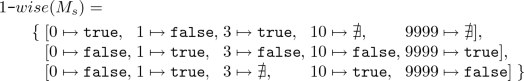
  With pair-wise testing, 12 samples can cover every pair of elements from different sets at least once.

4 Implementation

We implemented our automatic modeling approach for JavaScript because of its large number of builtin APIs and complex libraries, which are all opaque code for static analysis. They include the functions in the ECMAScript language standard [1] and web standards such as DOM and browser APIs. We implemented the modeling as an extension of SAFE  [13, 17], a JavaScript static analyzer. When the analyzer encounters calls of opaque code during analysis, it uses the SRA model of the code.

Sample. We applied the combinatorial sampling strategy for the SAFE abstract domains. Of the abstract domains for primitive JavaScript values, UInt, NUInt, and OtherStr represent an infinite number of concrete values (c.f. third case in Sect. 3.1) and thus require the use of heuristics. We describe the details of our heuristics and sample sets in Sect. 5.1.

We implemented the ${ Sample}$ step to use “each-used sample generation” for object abstract domains by default. In order to generate more samples, we added three options to apply pair-wise generation:

• ThisPair generates pairs between the values of this and heap,

• HeapPair among objects in the heap, and

• ArgPair among property values in an arguments object.

As an exception, we use the all-combination strategy for the DefaultDataProp domain representing a JavaScript property, consisting of a value and three booleans: writable, enumerable, and configurable. Note that field is used for language-independent objects and property is for JavaScript objects. The number of their combinations is limited to $2^3$. We consider a linear increase of samples as acceptable. The ${ Sample}$ step returns a finite set of concrete states, and each element in the set, which in turn contains concrete values only, is passed to the ${ Run}$ step.

Run. For each concrete input state, the ${ Run}$ step obtains a result state by executing the corresponding opaque code in four steps:

• 1. Generation of executable code

  First, ${ Run}$ populates object values from the concrete state. We currently omit the JavaScript scope-chain information, because the library functions that we analyze as opaque code are independent from the scope of user code. It derives executable code to invoke the opaque code and adds argument values from the static analysis context.

• 2. Execution of the code using a JavaScript engine

  ${ Run}$ executes the generated code using the JavaScript eval function on Node.js. Populating objects and their properties from sample values before invoking the opaque function may throws an exception. In such cases, ${ Run}$ executes the code once again with a different sample value. If the second sample value also throws an exception during population of the objects and their properties, it dismisses the code.

• 3. Serialization of the result state

  After execution, the result state contains the objects from the input state, the return value of the opaque code, and all the values that it might refer to. Also, any mutation of objects of the input state as well as newly created objects are captured in this way. We use a snapshot module of SAFE to serialize the result state into a JSON-like format.

• 4. Transfer of the state to the analyzer

  The serialized snapshot is then passed to SAFE, where it is parsed, loaded, and combined with other results as a set of concrete result states.

Abstract. To abstract result states, we mostly used existing operations in SAFE, like lattice-join, and also implemented an over-approximation heuristic function, ${ Broaden}$, comparable to widening. We use ${ Broaden}$ for property name sets in JavaScript objects, because ${ mayF}$ of a JavaScript abstract object can produce an abstract value that denotes an infinite set of concrete strings, and because $\Downarrow _{{ SRA}}$ cannot produce such an abstract value from simple sampling and join. Thus, we regard all possibly absent properties as sampled properties. Then, we implemented the ${ Broaden}$ function merging all possibly absent properties into one abstract property representing any property, when the number of absent properties is greater than a certain threshold proportional to a number of sampled properties.

5 Evaluation

We evaluated the model in two regards, (1) the feasibility of replacing existing manual models (RQ1 and RQ2) and (2) the effects of our heuristic H on the analysis soundness (RQ3). The research questions are as follow:

• RQ1: Analysis performance of

  Can $\Downarrow _{{ SRA}}$ replace existing manual models for program analysis with decent performance in terms of soundness, precision, and runtime overhead?

• RQ2: Applicability of

  Is $\Downarrow _{{ SRA}}$ broadly applicable to various builtin functions of JavaScript?

• RQ3: Dependence on heuristic H

  How much is the performance of $\Downarrow _{{ SRA}}$ affected by the heuristics?

After describing the experimental setup for evaluation, we present our answers to the research questions with quantitative results, and discuss the limitations of our evaluation.

5.1 Experimental Setup

In order to evaluate the model, we compared the analysis performance and applicability of with those of the existing manual models in SAFE. We used two kinds of subjects: browser benchmark programs and builtin functions. From 34 browser benchmarks included in the test suite of SAFE, a subset of V8 Octane¹, we collected 13 of them that invoke opaque code. Since browser benchmark programs use a small number of opaque functions, we also generated test cases for 134 functions in the ECMAScript 5.1 specification.

Each test case contains abstract values that represent two or more possible values. Because SAFE uses a finite number of abstract domains for primitive values, we used all of them in the test cases. We also generated 10 abstract objects. Five of them are manually created to represent arbitrary objects:

• OBJ1 has an arbitrary property whose value is an arbitrary primitive.

• OBJ2 is a property descriptor whose "value" is an arbitrary primitive, and the others are arbitrary booleans.

• OBJ3 has an arbitrary property whose value is OBJ2.

• OBJ4 is an empty array whose "length" is arbitrary.

• OBJ5 is an arbitrary-length array with an arbitrary property

The other five objects were collected from SunSpider benchmark programs by using Jalangi2 [20] to represent frequently used abstract objects. We counted the number of function calls with object arguments and joined the most used object arguments in each program. Out of 10 programs that have function calls with object arguments, we discarded four programs that use the same objects for every function call, and one program that uses an argument with 2500 properties, which makes manual inspection impossible. We joined the first 10 concrete objects for each argument of the following benchmark to obtain abstract objects: 3d-cube.js, 3d-raytrace.js, access-binary-trees.js, regexp-dna.js, and string-fasta.js. For 134 test functions, when a test function consumes two or more arguments, we restricted each argument to have only an expected type to manage the number of test cases. Also, we used one or minimum number of arguments for functions with variable number of arguments.

In summary, we used 13 programs for RQ1, and 134 functions with 1565 test cases for RQ2 and RQ3. All experiments were on a 2.9 GHz quad-core Intel Core i7 with 16 GB memory machine.

5.2 Answers to Research Questions

Answer to RQ1. We compared the precision, soundness, and analysis time of the SAFE manual models and the model. Table 1 shows the precision and soundness for each opaque function call, and Table 2 presents the analysis time and number of samples for each program.

As for the precision, Table 1 shows that produced more precise results than manual models for 9 (19.6%) cases. We manually checked whether each result of a model is sound or not by using the partial order function ($\sqsubseteq$) implemented in SAFE. We found that all the results of the SAFE manual models for the benchmarks were sound. The model produced an unsound result for only one function: Math.random. While it returns a floating-point value in the range [0, 1), modeled it as NUInt, instead of the expected Number, because it missed 0.

As shown in Table 2, on average $\Downarrow _{{ SRA}}$ took 1.35 times more analysis time than the SAFE models. The table also shows the number of context-sensitive opaque function calls during analysis (#Call), the maximum number of samples (#Max), and the total number of samples (#Total). To understand the runtime overhead better, we measured the proportion of elapsed time for each step. On average, ${ Sample}$ took 59%, ${ Run}$ 7%, ${ Abstract}$ 17%, and the rest 17%. The experimental results show that $\Downarrow _{{ SRA}}$ provides high precision while slightly sacrificing soundness with modest runtime overhead.

Answer to RQ2. Because the benchmark programs use only 15 opaque functions as shown in Table 1, we generated abstracted arguments for 134 functions out of 169 functions in the ECMAScript 5.1 builtin library, for which SAFE has manual models. We semi-automatically checked the soundness and precision of the $\Downarrow _{{ SRA}}$ model by comparing the analysis results with their expected results. Table 3 shows the results in terms of test cases (left half) and functions (right half). The Equal column shows the number of test cases or functions, for which both models provide equal results that are sound. The SRA Pre. column shows the number of such cases where the $\Downarrow _{{ SRA}}$ model provides sound and more precise results than the manual model. The Man. Uns. column presents the number of such cases where $\Downarrow _{{ SRA}}$ provides sound results but the manual one provides unsound results, and SRA Uns. shows the opposite case of Man. Uns. Finally, Not Comp. shows the number of cases where the results of $\Downarrow _{{ SRA}}$ and the manual model are incomparable.

Table 1. Precision and soundness by functions in the benchmarks

Table 2. Analysis time overhead by programs in the benchmarks

Table 3. Precision and soundness for the builtin functions

Table 4. Soundness and sampling cost for the builtin functions

The $\Downarrow _{{ SRA}}$ model produced sound results for 99.4% of test cases and 94.0% of functions. Moreover, $\Downarrow _{{ SRA}}$ produced more precise results than the manual models for 33.7% of test cases and 50.0% of functions. Although $\Downarrow _{{ SRA}}$ produced unsound results for 0.6% of test cases and 6.0% of functions, we found soundness bugs in the manual models using 1.3% of test cases and 7.5% of functions. Our experiments showed that the automatic $\Downarrow _{{ SRA}}$ model produced less unsound results than the manual models. We reported the manual models producing unsound results to SAFE developers with the concrete examples that were generated in the ${ Run}$ step, which revealed the bugs.

Answer to RQ3. The sampling strategy plays an important role in the performance of $\Downarrow _{{ SRA}}$ especially for soundness. Our sampling strategy depends on two factors: (1) manually sampled sets via the heuristic H and (2) each-used or pair-wise selection for object samples. We used manually sampled sets for three abstract values: UInt, NUInt, and OtherStr. To sample concrete values from them, we used three methods: Base simply follows the guidelines described in Sect. 3.1, Random generates samples randomly, and Final denotes the heuristics determined by our trials and errors to reach the highest ratio of sound results. For object samples, we used three pair-wise options: HeapPair, ThisPair, and ArgPair. For various sampling configurations, Table 4 summarizes the ratio of sound results, the average and maximum numbers of samples for the test cases used in RQ2.

The table shows that Base and Random produced sound results for 85.0% and 84.9% (the worst case among 10 repetitions) of the test cases, respectively. Even without any sophisticated heuristics or pair-wise options, $\Downarrow _{{ SRA}}$ achieved a decent amount of sound results. Using more samples collected by trials and errors with Final and all three pair-wise options, $\Downarrow _{{ SRA}}$ generated sound results for 99.4% of the test cases by observing more behaviors of opaque code.

5.3 Limitations

A fundamental limitation of our approach is that the $\Downarrow _{{ SRA}}$ model may produce unsound results when the behavior of opaque code depends on values that $\Downarrow _{{ SRA}}$ does not support via sampling. For example, if a sampling strategy calls the Date function without enough time intervals, it may not be able to sample different results. Similarly, if a sampling strategy does not use 4-wise combinations for property descriptor objects that have four components, it cannot produce all the possible combinations. However, at the same time, simply applying more complex strategies like 4-wise combinations may lead to an explosion of samples, which is not scalable.

Our experimental evaluation is inherently limited to a specific use case, which poses a threat to validity. While our approach itself is not dependent on a particular programming language or static analysis, the implementation of our approach depends on the abstract domains of SAFE. Although the experiments used well-known benchmark programs as analysis subjects, they may not be representative of all common uses of opaque functions in JavaScript applications.

6 Related Work

When a textual specification or documentation is available for opaque code, one can generate semantic models by mining them. Zhai et al. [26] showed that natural language processing can successfully generate models for Java library functions and used them in the context of taint analysis for Android applications. Researchers also created models automatically from types written in WebIDL or TypeScript declarations to detect Web API misuses [2, 16].

Given an executable (e.g. binary) version of opaque code, researchers also synthesized code by sampling the inputs and outputs of the code [7, 10, 12, 19]. Heule et al. [8] collected partial execution traces, which capture the effects of opaque code on user objects, followed by code synthesis to generate models from these traces. This approach works in the absence of any specification and has been demonstrated on array-manipulating builtins.

While all of these techniques are a-priori attempts to generate general-purpose models of opaque code, to be usable for other analyses, researchers also proposed to construct models during analysis. Madsen et al.’s approach [14] infers models of opaque functions by combining pointer analysis and use analysis, which collects expected properties and their types from given application code. Hirzel et al. [9] proposed an online pointer analysis for Java, which handles native code and reflection via dynamic execution that ours also utilizes. While both approaches use only a finite set of pointers as their abstract values, ignoring primitive values, our technique generalizes such online approaches to be usable for all kinds of values in a given language.

Opaque code does matter in other program analyses as well such as model checking and symbolic execution. Shafiei and Breugel [22] proposed jpf-nhandler, an extension of Java PathFinder (JPF), which transfers execution between JPF and the host JVM by on-the-fly code generation. It does not need concretization and abstraction since a JPF object represents a concrete value. In the context of symbolic execution, concolic testing [21] and other hybrid techniques that combine path solving with random testing [18] have been used to overcome the problems posed by opaque code, albeit sacrificing completeness [4].

Even when source code of external libraries is available, substituting external code with models rather than analyzing themselves is useful to reduce time and memory that an analysis takes. Palepu et al. [15] generated summaries by abstracting concrete data dependencies of library functions observed on a training execution to avoid heavy execution of instrumented code. In model checking, Tkachuk et al. [24, 25] generated over-approximated summaries of environments by points-to and side-effect analyses and presented a static analysis tool OCSEGen [23]. Another tool Modgen [5] applies a program slicing technique to reduce complexities of library classes.

7 Conclusion

Creating semantic models for static analysis by hand is complex, time-consuming and error-prone. We present a Sample-Run-Abstract approach ($\Downarrow _{{ SRA}}$) as a promising way to perform static analysis in the presence of opaque code using automated on-demand modeling. We show how $\Downarrow _{{ SRA}}$ can be applied to the abstract domains of an existing JavaScript static analyzer, SAFE. For benchmark programs and 134 builtin functions with 1565 abstracted inputs, a tuned $\Downarrow _{{ SRA}}$ produced more sound results than the manual models and concrete examples revealing bugs in the manual models. Although not all opaque code may be suitable for modeling with $\Downarrow _{{ SRA}}$, it reduces the amount of hand-written models a static analyzer should provide. Future work on $\Downarrow _{{ SRA}}$ could focus on orthogonal testing techniques that can be used for sampling complex objects, and practical optimizations, such as caching of computed model results.

References

ECMAScript Language Specification. Edition 5.1. http://www.ecma-international.org/publications/standards/Ecma-262.htm
Bae, S., Cho, H., Lim, I., Ryu, S.: SAFEWAPI: web API misuse detector for web applications. In: Proceedings of the 22nd ACM SIGSOFT International Symposium on Foundations of Software Engineering, pp. 507–517. ACM (2014)
Black, R.: Pragmatic Software Testing: Becoming an Effective and Efficient Test Professional. Wiley, Hoboken (2007)
Cadar, C., Sen, K.: Symbolic execution for software testing: three decades later. Commun. ACM 56(2), 82–90 (2013)
Ceccarello, M., Tkachuk, O.: Automated generation of model classes for Java PathFinder. ACM SIGSOFT Softw. Eng. Notes 39(1), 1–5 (2014)
Cousot, P., Cousot, R.: Abstract interpretation: a unified lattice model for static analysis of programs by construction or approximation of fixpoints. In: Proceedings of the 4th ACM SIGACT-SIGPLAN Symposium on Principles of Programming Languages, pp. 238–252. ACM (1977)
Gulwani, S., Harris, W.R., Singh, R.: Spreadsheet data manipulation using examples. Commun. ACM 55(8), 97–105 (2012)
Heule, S., Sridharan, M., Chandra, S.: Mimic: computing models for opaque code. In: Proceedings of the 2015 10th Joint Meeting on Foundations of Software Engineering, pp. 710–720. ACM (2015)
Hirzel, M., Dincklage, D.V., Diwan, A., Hind, M.: Fast online pointer analysis. ACM Trans. Program. Lang. Syst. (TOPLAS) 29(2), 11 (2007)
Jha, S., Gulwani, S., Seshia, S.A., Tiwari, A.: Oracle-guided component-based program synthesis. In: Proceedings of the 32nd ACM/IEEE International Conference on Software Engineering, vol. 1, pp. 215–224. ACM (2010)
Kuhn, D.R., Wallace, D.R., Gallo, A.M.: Software fault interactions and implications for software testing. IEEE Trans. Softw. Eng. 30(6), 418–421 (2004)
Lau, T., Domingos, P., Weld, D.S.: Learning programs from traces using version space algebra. In: Proceedings of the 2nd International Conference on Knowledge Capture, pp. 36–43. ACM (2003)
Lee, H., Won, S., Jin, J., Cho, J., Ryu, S.: SAFE: formal specification and implementation of a scalable analysis framework for ECMAScript. In: FOOL 2012: 19th International Workshop on Foundations of Object-Oriented Languages, p. 96. Citeseer (2012)
Madsen, M., Livshits, B., Fanning, M.: Practical static analysis of JavaScript applications in the presence of frameworks and libraries. In: Proceedings of the 2013 9th Joint Meeting on Foundations of Software Engineering, pp. 499–509. ACM (2013)
Palepu, V.K., Xu, G., Jones, J.A.: Improving efficiency of dynamic analysis with dynamic dependence summaries. In: Proceedings of the 28th IEEE/ACM International Conference on Automated Software Engineering, pp. 59–69. IEEE Press (2013)
Park, J.: JavaScript API misuse detection by using TypeScript. In: Proceedings of the Companion Publication of the 13th International Conference on Modularity, pp. 11–12. ACM (2014)
Park, J., Ryou, Y., Park, J., Ryu, S.: Analysis of JavaScript web applications using SAFE 2.0. In: 2017 IEEE/ACM 39th International Conference on Software Engineering Companion (ICSE-C), pp. 59–62. IEEE (2017)
Păsăreanu, C.S., Rungta, N., Visser, W.: Symbolic execution with mixed concrete-symbolic solving. In: Proceedings of the 2011 International Symposium on Software Testing and Analysis, pp. 34–44. ACM (2011)
Qi, D., Sumner, W.N., Qin, F., Zheng, M., Zhang, X., Roychoudhury, A.: Modeling software execution environment. In: 2012 19th Working Conference on Reverse Engineering (WCRE), pp. 415–424. IEEE (2012)
Sen, K., Kalasapur, S., Brutch, T., Gibbs, S.: Jalangi: a selective record-replay and dynamic analysis framework for JavaScript. In: Proceedings of the 2013 9th Joint Meeting on Foundations of Software Engineering, pp. 488–498. ACM (2013)
Sen, K., Marinov, D., Agha, G.: CUTE: a concolic unit testing engine for C. In: ACM SIGSOFT Software Engineering Notes, vol. 30, pp. 263–272. ACM (2005)
Shafiei, N., Breugel, F.V.: Automatic handling of native methods in Java PathFinder. In: Proceedings of the 2014 International SPIN Symposium on Model Checking of Software, pp. 97–100. ACM (2014)
Tkachuk, O.: OCSEGen: open components and systems environment generator. In: Proceedings of the 2nd ACM SIGPLAN International Workshop on State Of the Art in Java Program Analysis, pp. 9–12. ACM (2013)
Tkachuk, O., Dwyer, M.B.: Adapting side effects analysis for modular program model checking, vol. 28. ACM (2003)
Tkachuk, O., Dwyer, M.B., Pasareanu, C.S.: Automated environment generation for software model checking. In: Proceedings of the 18th IEEE International Conference on Automated Software Engineering, pp. 116–127. IEEE (2003)
Zhai, J., Huang, J., Ma, S., Zhang, X., Tan, L., Zhao, J., Qin, F.: Automatic model generation from documentation for Java API functions. In: 2016 IEEE/ACM 38th International Conference on Software Engineering (ICSE), pp. 380–391. IEEE (2016)
Acknowledgment
This work has received funding from National Research Foundation of Korea (NRF) (Grants NRF-2017R1A2B3012020 and 2017M3C4A7068177).
Author information
Authors and Affiliations
Corresponding authors
Editor information
Editors and Affiliations
Rights and permissions
Open Access This chapter is licensed under the terms of the Creative Commons Attribution 4.0 International License (http://creativecommons.org/licenses/by/4.0/), which permits use, sharing, adaptation, distribution and reproduction in any medium or format, as long as you give appropriate credit to the original author(s) and the source, provide a link to the Creative Commons license and indicate if changes were made.
The images or other third party material in this chapter are included in the chapter's Creative Commons license, unless indicated otherwise in a credit line to the material. If material is not included in the chapter's Creative Commons license and your intended use is not permitted by statutory regulation or exceeds the permitted use, you will need to obtain permission directly from the copyright holder.
Copyright information
© 2019 The Author(s)
About this paper
Cite this paper
Park, J., Jordan, A., Ryu, S. (2019). Automatic Modeling of Opaque Code for JavaScript Static Analysis. In: Hähnle, R., van der Aalst, W. (eds) Fundamental Approaches to Software Engineering. FASE 2019. Lecture Notes in Computer Science(), vol 11424. Springer, Cham. https://doi.org/10.1007/978-3-030-16722-6_3
Download citation
DOI: https://doi.org/10.1007/978-3-030-16722-6_3
Published:
Publisher Name: Springer, Cham
Print ISBN: 978-3-030-16721-9
Online ISBN: 978-3-030-16722-6
eBook Packages: Computer ScienceComputer Science (R0)