
Abstract
With the development of 3D GIS technology, the application of 3D GIS in agriculture has become a hotspot in agricultural information technology research. A total of 109 soil samples were collected from the soil of Jilin Province Yushu City Gongpeng Town No. 13 Village No. 7 test area. Three - dimensional visualization of soil nutrient evolution in maize precise operation area was carried out by using ArcGIS technology. Firstly, the Kriging optimal interpolation method was used to calculate the sampling points of soil nutrient space in the field of maize test field. Then three-dimensional spatial map of soil available phosphorus, available potassium available nitrogen and other nutrient contents during the period from 2005 to 2009 were established by using the spatial analysis technique of 3D GIS. By comparing its three-dimensional thematic map, analyze trends in the evolution of its soil fertility characteristics. The results showed that the difference of soil fertility was gentle after four years of variable fertilization, and the effect of precision fertilization was verified.
You have full access to this open access chapter, Download conference paper PDF
1 Introduction
With the development of computer science and 3D simulation technology, the development and application of 3D GIS are becoming more and more mature. 3D GIS can truly perceive the objective world, present the spatial geography phenomenon to the user, and carry on the three-dimensional spatial analysis operation to the space object. However, the current three-dimensional GIS in the field of agricultural applications less [1]. Therefore, this study in the national “863” project demonstration base in Yushu City Gongpeng Town No. 13 Village No. 7 test area by 40 m * 40 m grid sampling. The soil nutrient content was measured and the characteristics of soil nutrient evolution were discussed by using the three-dimensional GIS spatial analysis technique. The spatial variation of soil nutrient after precision fertilization was analyzed and analyzed, which provided a reliable basis for the division of farmland precision management area and Implementation of Precise Operation of Corn [2].
2 Materials and Methods
2.1 Overview of the Study Area
The study area is the experimental field of the NO. 13th village of Gongpeng Town, Yushu City, Jilin Province. It is located in the eastern part of Jilin Province and is a semi-humid temperate continental monsoon climate. It is characterized by four distinct seasons, winter long summer short, annual precipitation in the 500–600 mm, the vast majority of concentrated in the warm season, accounting for about 90% of annual precipitation, the annual average temperature of 4.6–5.6 °C. Soil type is a typical black soil, the main crop is corn and soybeans, etc. It is an important commodity grain base in Jilin Province [3, 4].
In the national “863” project “Research and Application of Corn Precision Operation System” and the national Spark plan “Integration and Demonstration of Precision Training Technology of Corn Based on Internet of Things and demonstration of” the strong support of the project in Yushu City Gongpeng Town No.13 Village continuous four years of variable fertilization operations, the accumulation of a large number of soil nutrient space data. Therefore, this article selected the Yushu City Gongpeng Town No.13 Village No. 7 plots were experimented and research. The total area of the test field is about 375 mu, and the grid size is set to A1~L11 as the sampling point [5]. We selected the three kinds of nutrient data of available phosphorus, available nitrogen and available potassium respectively, and the application of the algorithm for four years of continuous variable fertilization from 2005 (before variable fertilization) to 2009 on the Yushu City Gongpeng Town No. 13 Village No. 7 plots.
2.2 Data Collection
Application of GPS (Global Satellite Differential Positioning System) device for precise positioning, the use of ArcGIS software to produce the soil grid sampling map, sample distribution shown in Fig. 1.

Sampling grid diagram
2.3 Research Methods
In this paper, the Kriging optimal interpolation method was used to calculate the sampling points of soil nutrient space in the field of maize experiment field. On this basis, the three-dimensional visualization of soil nutrient multidimensional spatial data was realized by regular body element model. Through the three-dimensional Kriging interpolation algorithm, the original data contained in the spatial distribution of features without significant loss of the situation first passed to the estimated grid points other than the unknown data, so that the structure of the three-dimensional space model more realistic real soil environment. The three-dimensional Kriging interpolation method is essentially an improved score for the inverse distance weighting method, but it is still a linear interpolation method [6]. The principle of Kriging interpolation is that the attribute Z(x) at the point \( {\text{Xi}} \in {\text{A }}\left( {{\text{i}} = \, 1, \, 2, \, \ldots ,{\text{ n}}} \right) \) is Z(Xi), the interpolated point \( {\text{X0}} \in {\text{A}}\left( {\text{X0}} \right) \), the Kriging interpolation result Z*(X0) is the weighted sum of the known sampling point attribute values Z(Xi) (i = 1, 2, …, n).
(1) where λi is the weight coefficient of the attribute value to be determined. There is a certain correlation between Z(Xi), which is related to the distance, but also to its relative direction change. Thus, the three-dimensional Kriging method refers to the object of study as a regionally controllable amount of change. We obtain the matrix of coefficient coefficients of the attribute value Kriging by using the spherical model, and then determine the augmented matrix for the spatial position of each unknown point. We obtain the weight coefficient value by solving the Kriging equation group, and then we can get each. The estimated value of the attribute value and the estimated variance of the attribute value.
2.4 3D GIS Spatial Analysis Technique
2.4.1 Information Acquisition
The spatial data of sampling points in 2005, 2007 and 2009 were obtained by GPS respectively and the data of the soil samples of the sampling points were obtained as shown in Table 1 (Tables 2 and 3).
2.4.2 ArcScene Three-Dimensional Model of the Establishment
Firstly, the attribute information of available phosphorus, available nitrogen and available potassium in the soil of Gongpeng Town in Yushu City of Jilin Province in 2005, 2007 and 2009 were transformed into spatial information. Then, the Kriging interpolation method is used to calculate the element values of the points in the three-dimensional space in the region. On the basis of this, the 3D visualization of soil element data is realized by ArcScene.
-
(1)
First open the ArcScene module, the ArcMap in the two-dimensional data (Fig. 2) into the ArcScene, while loading DEM data (Fig. 3).
Fig. 2. 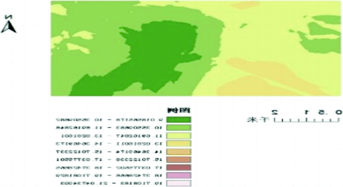
2D spatial variation of available phosphorus in 2005
Fig. 3. 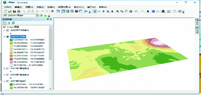
Two-dimensional model after registration in ArcMap
-
(2)
Now, the DEM or two-dimensional. Then find the left side of the layer file, right click to open a drop down menu. Click “Properties”, a pop-up “Layer Properties” dialog box, as shown in Fig. 4.
Fig. 4. 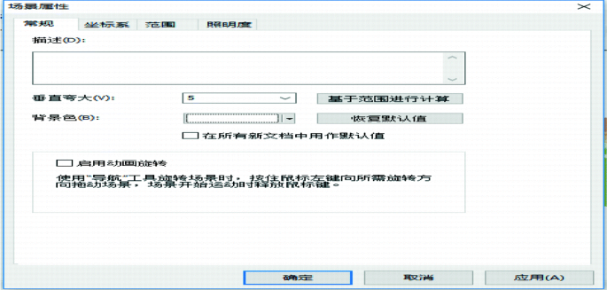
Layer Properties
-
(3)
In the “Elevation from Surface”, select “Float on a custom surface” (the surface here is itself). You can find click “OK”, DEM did some changes, but this is not very obvious.
-
(4)
Then click on the “Scene layer”, select the “scene properties” option (Fig. 5), opened a “scene properties” menu. Here you can adjust the value of “vertical exaggerated” and set it to 5. Now you can see, the DEM’s three-dimensional sense has been very strong.
Fig. 5. 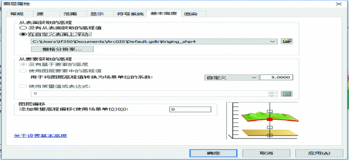
Scene property
-
(5)
Change the color of the model, and then in step 2 to open the “layer properties”, the color is set to eye-catching color (Fig. 6). So that the completion of the three-dimensional model [7].
Fig. 6. 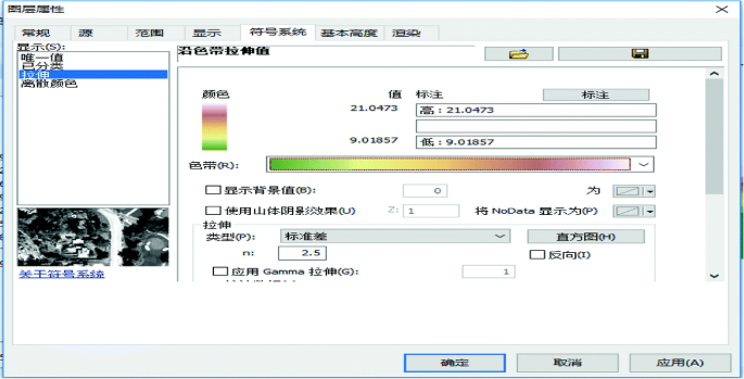
Stretch


From Figs. 7, 8 and 9, it is the three-dimensional spatial distribution of available nitrogen, available phosphorus and available potassium in soil nutrients of groundwater No. 7 and the historical evolution of soil nutrient content can be analyzed according to these historical data [8].

Spatial variability of available phosphorus in 2005–2009

Spatial variability of available Potassium in 2005–2009

Spatial variability of available nitrogen in 2005–2009
3 The Results and Analysis
It can be seen from Figs. 7, 8 and 9 that the nutrient content of soil is gradually increased with the implementation of variable fertilization [9, 10]. The available nitrogen content increased from 121.15 mg/kg in 2005 to 139.31 mg/kg in 2009, and the available phosphorus content increased from 12.20 mg/kg in 2005 to 21.07 mg/kg in 2009, and the available potassium content increased from 113.95 mg/kg in 2005 to 137.89 mg/kg in 2009. As the amount of fertilizer to phosphate-based, so in the individual years of available nitrogen and available potassium content is not much change. At the same time, with the implementation of variable fertilization techniques, the difference of soil available nutrient content in different years was gradually reduced, which was probably due to the slow release of soil available phosphorus and available potassium in soil. The results show that the implementation of variable fertilization technology, while improving the soil fertility, but also promote the soil fertility balance, is conducive to the correct evaluation of soil fertility changes.
4 Conclusion
-
(1)
3D GIS (Figs. 7, 8 and 9) can show more information than the two-dimensional spatial variation map (Fig. 2), and the spatial variation of soil available nutrient is more clear, Intuitive and true.
-
(2)
The high degree of data change in the three-dimensional spatial variation map can fully prove the significant effect of variable fertilization in 2005 and 2009, which is beneficial to the correct evaluation of soil fertility change.
-
(3)
Three-dimensional visualization technology can not only be applied to the three-dimensional distribution of soil nutrient spatial distribution, which can let users experience the spatial distribution characteristics of real soil nutrient, which is beneficial to soil fertility analysis and evaluation, but also the soil nutrient three-dimensional spatial variation map for any mobile, rotation, split and extraction operations. The process and results of variable fertilization are tested and forecasted, which provides an objective, image and reliable auxiliary decision tool.
References
Wang, X., Wu, D., Wang, Z.: Study on dynamic monitoring of basic farmland based on GPS and GIS technology. J. Urban Surv. 05, 13–15 (2013)
Wang, H., Li, D., Hou, Z., Lu, X.: Spatial and temporal variability of soil nutrients in farmland based on GIS. Xinjiang Agric. Sci. 10, 1872–1878 (2013)
Zhao, Y., Chen, G., Wang, Y.: Study on spatial variability of soil nutrients based on GIS. Northwest Agric. Sci. 6, 195–198 (2005)
Jiang, J.: Based on the spatial fuzzy clustering of visual variable fertilization decision-making system. Jilin Agricultural University (2011)
Zhao, Y., Wang, Y., Han, H., Chen, G.: Spatial variation of soil nutrients in typical black soil region of Jilin province. China Agric. Mechanization 2, 72–75 (2012)
Jiang, J., Chen, G.: Study and realization of three-dimensional visualization of soil nutrients based on VTK. Agric. Netw. Inf. 03, 10–13 (2011)
Qin, L.P.: ArcScene campus three-dimensional scene of the establishment. Chin. Names 06, 78–79 (2014)
Lu, X., Ma, W., Wei, X.: Spatial variability of soil fertility in agricultural science and technology demonstration park supported by GIS technology. J. Zhejiang Agric. Sci. 03, 3–6 (2004)
Chen, H., Cao, L., Chen, G.: Study and application of temporal and spatial variability of soil fertility. J. Chin. Soc. Agric. Mechanization 04, 268–273 (2014)
Hu, S., Li, K.: Three-dimensional GIS key technology research. Geospat. Inf. 03, 9–12 (2008)
Acknowledgments
This work was funded by the China Spark Program. 2015GA66004. “Integration and demonstration of corn precise operation technology based on Internet of things”.
Funding
The national spark program project: Precise operation technology integration and demonstration of corn (No. 2015GA660004).
Author information
Authors and Affiliations
Corresponding author
Editor information
Editors and Affiliations
Rights and permissions
Copyright information
© 2019 IFIP International Federation for Information Processing
About this paper

Cite this paper
Xiao, E., Chen, G., Zhao, S., Fu, S. (2019). Three - Dimensional Visualization of Soil Nutrient Evolution in Maize Precision Operation Area Based on ArcGIS. In: Li, D., Zhao, C. (eds) Computer and Computing Technologies in Agriculture XI. CCTA 2017. IFIP Advances in Information and Communication Technology, vol 546. Springer, Cham. https://doi.org/10.1007/978-3-030-06179-1_13
Download citation
DOI: https://doi.org/10.1007/978-3-030-06179-1_13
Published:
Publisher Name: Springer, Cham
Print ISBN: 978-3-030-06178-4
Online ISBN: 978-3-030-06179-1
eBook Packages: Computer ScienceComputer Science (R0)