
Abstract
This section focusses on the dynamic modelling of the machine tool including its computer numeric control. To properly simulate modern machine tools in machining condition, which show close interaction between the dynamic behaviour of the mechanical structure, drives, and the CNC, we use an integrated methodology that combines control and MBS capabilities in a nonlinear FEA solver called SAMCEF Mecano. The capacity of such digital twin model to simulate machine tool dynamics is demonstrated considering several validation tests.
You have full access to this open access chapter, Download chapter PDF
Keywords
1 Introduction
The virtual prototype of a machine tool is a computer simulation model of the physical product that can be presented, analysed and tested like a real machine. The technology included in such a virtual prototype covers several engineering fields and tools depending on the stage of the design process or the studied manufacturing process. A complete review of Virtual Machine Tool technology is available in [1].
Modern machine tools are very complex mechatronic systems. The capability and efficiency of a machine tool are mainly determined by its kinematics, structural dynamics, computer numerical control system and the machining process. The kinematics is usually analysed by means of rigid multibody simulation tools (MBS) based on a 3D CAD model of the machine [2]. The finite element analysis (FEA) is used to calculate static stiffness or dynamic characteristics of the machine tool, e.g. natural frequencies and mode shapes [3]. 1D-CAE functional tools are efficiently used for computer numerical control systems [4] and actuation, while very dedicated commercial and research tools are used for cutting processes [5].
New highly dynamic machine requires high static and dynamic stiffness to ensure machining accuracy and high dynamic properties of the feed drive to decrease the manufacturing time. This is achieved by employing small moving masses with sufficient stiffness of the structural parts and high adjustable controller parameters of the drives. This leads to interactions between structural dynamics and feed drive controls, which have to be considered in the simulations [6, 7]. Natural frequencies of the feed drives are coupled with lower natural frequencies of the machine structure. To avoid instabilities, the control parameters have to be reduced, which leads to a limitation of the productivity of the machine tool.
The methodology proposed in Twin-Control is considering these interactions from the early design stage of the machine to the virtual prototyping verifications. The best method to couple structural dynamic and control loops is the flexible multibody approach. In this case, the components of the machine tool can represent the static as well as the dynamic behaviour. Those flexible components are introduced in flexible multibody system (MBS) simulation tool as super-elements created by modal reduction of detailed FEA models. The different elements which are used to connect the structural components, such as guiding systems, mounting devices or ball screw drives, are modelled as a combination of flexible connectors and flexible joints depending on the specific configuration.
The coupling with the control loops is achieved by co-simulation with 1D-CAE functional models. Most of 1D-CAE tools offer the possibility to embed the model of the control loop in some dynamic libraries (DLL). On the other side, MBS tools have interfaces or special elements that can use such DLL as a slave process and close the control loop providing velocities and displacements of the axes and receiving driving forces.
In the Twin-Control system, all this is achieved using the SAMCEF Mecano solver coupled with MATLAB/Simulink. As SAMCEF Mecano [8] is an implicit nonlinear FEA solver with MBS capabilities [9], this solution can be used from early concept design (machine kinematic) to virtual prototyping, including all FEA analyses made for components design and verification. Moreover, the finite element approach of MBS simulation is more efficient when many flexible components are considered within a large frequency range. In this case, because of extensive use of super-elements, the flexible MBS system can become unusually large for MBS solvers, but are still quite small for a FEA solver.
2 The Virtual Machine Tool Concept
Within the scope of the Twin-Control project, the VMT concept was used to model two machines, a high-speed 4 axes box-in-box machine from Comau and a large 3 spindles five axes machine from Gepro (Fig. 3.1).

Virtual machine tool models developed in Twin-Control project: a Comau Urane 25V3 machine, b Gepro 502 machine
2.1 Structural Model
To fully model the dynamic behaviour of a machine tool when operating, the following objectives are followed:
-
Fully account for the flexibility of all structural components, connections and feed drive to obtain a model that can represent vibrations inside the machine.
-
Limit the number of degrees of freedom to as few as possible to allow for efficient time domain simulation (small time step imposed mainly by the machining simulation module and the controller model).
Usually, a machine is made of several main structural frames, which are modelled using the super-element technique. The selected modal contains of the super-elements allow considering vibrations up to a desired frequency range. Non-structural masses are added to the moving frames to properly account for all moving components as motors, lubrication and cooling systems, etc., which are not considered in the mechanical model. Figure 3.2 shows the mesh used to create the super-element corresponding to one of the “support leg” of the Gepro machine. Ones can see the spider connections that link the retained nodes to the structure.

FE model for super-element creation (leg of the Gepro machine)
The guiding system for translational motion between two frames is based on sliders. Modelling such devices requires a flexible slider element, which constrains a node to move along a deformable trajectory represented by a beam element. As the track is part of the structural frame model, fictive beams are used to connect the slider nodes to the retained node of the super-element, considering its stiffness inside the slider element. The skates are idealized by the sliding node and an associated bushing that characterizes its stiffness and damping.
2.2 Drive Train
If the machine is driven by pairs of linear motors as in the case of Comau machine, it is modelled by pairs of flexible sliders defined from the frame super-elements retained nodes. As the role of those sliders is to transfer axial forces, and not to contribute to the guiding function, the bushing associated with the sliding node has only axial stiffness. For those sliders, the sliding DOF can be force-driven by the controller model.
For drive systems including conventional motors, screw, rack–pinions, or other transmission systems, like in the Gepro machine, a library of simplified components models is used. An example is given for the driving system of the X-axis of Gepro’s machine (highlighted in Fig. 3.1), which is made of four rack–pinion connections individually driven by a rotational motor and a gearbox.
Figure 3.3 shows a schematic view of this model, where blue nodes are structural components, green arrows kinematical dofs, orange cylinders represents masses and inertia, CNLI boxes are kinematical constraints, K boxes local stiffness, and red points belongs to the table (slider).

Schematic view of the feed drive model (X-axis of the Gepro machine)
The green box is the motor model, it is a “scalar model” with only one rotation dof per node; flexible coupling is considered as part of the motor. The torsional stiffness K1 is introduced between input and output nodes, while all rotating inertias associated with the motor shaft are applied on the output node. The motor mass is reported to a structural node of the gearbox model. The red box represents the gearbox. The CNLI constraint account for the reduction factor, it relates the motor shaft dof to the output shaft of the gearbox. The gearbox output shaft is modelled by two coincident nodes connected to the “leg” structure by two hinge joints of y-axis. Those two nodes are also linked by the K2 torsional stiffness of the gearbox with respect to the output shaft. The torsional inertia associated with the output shaft of the gearbox is defined in the mass and inertia element associated with node named “Pinion shaft”, which also include the mass of the whole system. The rotational dof of the gearbox output shaft is driven from the linear constraint (CNLI box) that imposes the reduction factor, while pinion rotational dof is used to constraint the sliding dof on the rack (red nodes) with the second linear constraint. This is done in the blue box that manages the rack–pinion interaction. The coefficient of the linear constraint is the primitive radius of the pinion. This model is repeated for each of the four motors associated with this X-axis.
2.3 Spindle Model
The spindle is a crucial component of the machine, which should be accounted in the mechanical model. From the structural point of view, it is made of housing, a shaft and a set of bearings (see Fig. 3.4).

Spindle CAD model
In the VMT approach, the shaft is not rotating, and tool spinning is considered in the machining module. In our models, the spindle rotor is idealized by a set of beam elements. Those are connected to the structure (super-element) by a set of bearing elements. The integrated model is shown in Fig. 3.5.

Spindle beam model in the Comau machine
2.4 Modelling Principle
To summarize, the modelling process based on the CAD model of the machine is the following:
-
Create/import the CAD model of the machine in the modelling environment (Simcenter).
-
Create FE models of the structural components.
-
Create super-elements from those models retaining the nodes needed for the connections.
-
Import super-elements in the simulation environment (SAMCEF Mecano used as MBS solver) as shown in Fig. 3.6. If CAD models of the components are extracted from the global CAD model of the machine, the super-element created from those are at correct positions.
Fig. 3.6 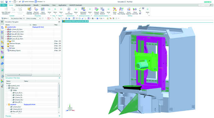
Definition of a machine tool in Simcenter for Samcef
-
Connect the structural components with flexible joints.
-
Model drive trains, sensing systems, motors, etc.
-
Include CNC model (Simulink model imported as a DLL in the mechanical model), and link to the CNC the axes position set point, which are the boundary conditions of the model.
-
Use the dedicated TOOL element of Mecano to couple the VMT with the machining force module.

2.5 Control
For each axis, there are one or two rulers measuring the relative motion between two successive frames. These measurements are used as inputs to the controller and to compare against nominal axis motions. The rulers are represented in the model by sensor elements that associate measures in the model to some nodal DOF that can be connected to the controller model.
Most of CNC (Siemens 840D for the Comau machine and Fagor 8070 for the Gepro machine) have a similar architecture, and the main components of controller model are:
-
Position, velocity and current feedback control loops;
-
Velocity and acceleration feedforward;
-
Power stage and motor models;
-
Filters;
-
Current set-point filters.
A simplified version of the control model was developed [10], disregarding the effect of current control loop and filters. Proper inputs and outputs are added to connect the mechanical model. Also, specific systems such as the pre-load loop are integrated to adapt to specific machine axes. This adapted Simulink model (see Fig. 3.7) is translated into a dynamic library and associated with a specific control element of SAMCEF Mecano that is used to manage the coupling between 1D model (control) and the full flexible 3D model (machine).

CNC model for rack drive with 2 motors (X-axis of Gepro 502 machine)
3 Validation of the VMT
The validation test procedure is presented focusing on the Comau machine. Models are validated considering two types of tests. First, hammer tests are done in six machine configurations (see Fig. 3.8). Obtained frequency response function (FRF) at the spindle tip position in the three main directions is checked to verify modal frequencies of the structure and to tune the structural damping. Secondly, the model driven by its controller is used to impose quick uniaxial motion. Model results are compared with experimental data obtained in real machines from the CNC monitoring. Some validation examples are shown in the next section for the Comau box-in-box machine.

Machine configurations
3.1 Hammer Test (Comau Machine)
Most of the tests are done hitting the extremity of the spindle frame, having the accelerometer at the same localization. For some configurations, tests have been performed hitting also on a tool holder, while measuring acceleration on it. This allows exciting not only the structure modes, but also the spindle modes. In the models, excited nodes are located either on the frame super-element or at the extremity of the spindle beam (see Figs. 3.5 and 3.9).

Hammer test on z-frame and tool (spindle tip)
The modelling of a hammer test can be performed either in the frequency or the time domain. In the first approach, the flexible MBS model is used to position the machine in the desired configuration, and the solver exports its linearized matrices that are used to perform a harmonic response on the frequency range of interest. For this analysis, a unitary force is applied on the hammer impact position, resulting acceleration at the measurement point is monitored to obtain the desired FRF function. Modal damping is introduced to tune the magnitude of the excited modes. For the time domain simulation, the machine is positioned in the test configuration, and a constant force impact is applied during 1 ms. The one-second interval after the impact is simulated, and the acceleration signal is stored. The FRF is then obtained by dividing the fast Fourier transform (FFT) of the measured acceleration by the FFT of the applied force. Some simulation results are compared to the test measurements for configuration 1, which is representative of all other configurations (Fig. 3.10).

FRF (X-direction magnitude in g/N) computed by harmonic response, by time domain simulation and measured values
Both numerical models exhibit two main peaks close to 110 and 260 Hz that corresponds to the measurement within a 10% error margin. Frequency and time domain responses show small discrepancies in resonance locations because of different representations of the CNC, damping models are also different in both modelling approaches. The experimental curve presents “noise” in the frequency range above 300 Hz, and this behaviour is approached by the model. For harmonic response, the magnitudes at the resonances are easily tuned from the definition of modal damping. The management of damping in time domain simulation is less flexible. However, it was possible to approach resonance magnitudes by adjusting structural damping in the super-elements and inside the ground fixations.
Higher natural frequencies related to the spindle dynamics are observed depending on the direction of the impact and the measure. Results from the model are compared to the validation test data in Table 3.1.
The simulated frequencies match quite well the experimental results. Resonance magnitudes show less agreement, probably due to the FRF computation process and a lack of damping characterization in the spindle model. Notice that modes simulated for the test in the transverse directions (x and y) are perfectly symmetric, which is not in the case in real machine.
3.2 Fast 1 Axis Motion (Comau Machine)
The purpose of this second type of test is to validate the simulation while the machine and its controller interact. Considering real machine dynamic restrictions (maximum jerk, acceleration and velocity), the quickest 100 mm displacement along the Y-axis is generated and fed as a time function to the controller model, which also gets from the machine model the position and velocity along the ruler of the considered machine axis. The controller model of Fig. 3.7 is, then, able to impose forces on the dof of the sliders representing the two linear motors driven by this control loop. CNC model provides also positioning and velocity errors.
Figures 3.11 and 3.12 show axis motion (position, velocity and positioning error) resulting from the force applied by the linear motors. The machine is almost perfectly driven by the CNC, with maximal positioning error limited to 28 microns during acceleration phases. This is the same as the data recorded by the physical CNC during the manoeuver (Fig. 3.13). Computed axis velocity is also in close agreement with experimental measures. Because the simplified CNC model does not include the current loop, current is not available from the model. However, the force applied in the linear motor has the same shape as the current curve of Fig. 3.13.

Y-axis position and positioning error during simulation of the positioning test

Y-axis velocity and motor force during simulation of the positioning test

Record of the CNC during real positioning test
The upper graph recorded by the CNC (Fig. 3.13) presents the requested position and the associated positioning error. The bottom graph presents the velocity and applied current inside the linear motor, which is proportional to the generated force.
4 Conclusions
In this section, a methodology for virtual prototyping of machine tool is presented. The proposed technology has been applied to build mechatronic flexible multibody models of several machines. The virtual machine tool can be coupled to a cutting force module. This modelling approach is of key importance to provide comprehensive simulations capabilities for virtual machine tool prototyping in working conditions. The resulting Twin-Control simulation package, which includes the VMT concept, is intended for both machine tool builders for design activities and machine tool users to improve their processes. In both cases, this virtual model can be used to avoid performing costly physical tests.
References
Altintas, Y., Brecher, C., Weck, M., Witt, S.: Virtual machine tool. CIRP Ann.—Manufact. Technol. (2005)
Weule, H., Albers, A.., Haberkern, A., Neithardt, W., Emmrich, D.: Computer aided optimisation of the static and dynamic properties of parallel kinematics. In: Proceedings of the 3rd Chemnitz Parallel Kinematic Seminar, pp. 527–546 (2002)
Cook, R., Malkus, D., Plesha, M.: Concepts and Applications of Finite Element Analysis, 3rd edn. Wiley, Madison (1988)
Prévost, D., Lavernhe, S., Lartigue, C.: Feed drive simulation for the prediction of the tool path follow up in high speed machining. J. Mach. Eng. High Perform. Manuf.—Mach. 8(4), 32–42 (2008)
Schmidt, J., Söhner, J.: Use of FEM simulation in manufacturing technology. In: ABAQUS Users’ Conference, Newport, RI, USA, 29–31 May 2002
Ghassempouri, M., Vareilles, E., Fioroni, C.: Modelling and simulating the dynamic behavior of a high speed machine tool. In: Samtech Users Conference (2003)
Morelle, P., Granville, D., Goffart, M.: SAMCEF for Machine Tools resulting from the EU MECOMAT project. In: NAFEMS Seminar—Mechatronics in Structural Analysis, Wiesbaden, Germany, May 2004
Samtech: SAMCEF V18.1 User Manual (2017)
Géradin, M., Cardona, A.: Flexible Multi-body Dynamics: A Finite Element Approach. Willey, New York (2001)
Cugnon, F., Ghassempouri, M., Armendia, M.: Machine tools mechatronic analysis in the scope of EU Twin-Control project. In: Nafems World Conference, Stockholm, Sweden, June 2017
Author information
Authors and Affiliations
Corresponding author
Editor information
Editors and Affiliations
Rights and permissions
Open Access This chapter is licensed under the terms of the Creative Commons Attribution 4.0 International License (http://creativecommons.org/licenses/by/4.0/), which permits use, sharing, adaptation, distribution and reproduction in any medium or format, as long as you give appropriate credit to the original author(s) and the source, provide a link to the Creative Commons license and indicate if changes were made.
The images or other third party material in this chapter are included in the chapter's Creative Commons license, unless indicated otherwise in a credit line to the material. If material is not included in the chapter's Creative Commons license and your intended use is not permitted by statutory regulation or exceeds the permitted use, you will need to obtain permission directly from the copyright holder.
Copyright information
© 2019 The Author(s)
About this chapter

Cite this chapter
Cugnon, F., Ghassempouri, M., Etxeberria, P. (2019). Virtualization of Machine Tools. In: Armendia, M., Ghassempouri, M., Ozturk, E., Peysson, F. (eds) Twin-Control. Springer, Cham. https://doi.org/10.1007/978-3-030-02203-7_3
Download citation
DOI: https://doi.org/10.1007/978-3-030-02203-7_3
Published:
Publisher Name: Springer, Cham
Print ISBN: 978-3-030-02202-0
Online ISBN: 978-3-030-02203-7
eBook Packages: EngineeringEngineering (R0)