Ramsey Model

Abstract

This chapter presents the Ramsey model. It is the benchmark model for most dynamic macroeconomic models that study growth and business cycle phenomena. We first study the deterministic Ramsey model in which the total factor productivity is certain. We contrast the effects of a once-and-for-all change with those of a temporary change in productivity on investment, output, and labor supply. In addition, we distinguish the effects of this change when it is known in advance or only observed at the beginning of the period, t, when the shock occurs. Finally, we also introduce uncertainty with respect to the technology level and discuss the real business cycle (RBC) model.

Appendices

Appendix 2.1: Intertemporal Elasticity of Substitution and Savings

1.1 Derivation of the Intertemporal Elasticity of Substitution

In this appendix, we derive an expression for the intertemporal elasticity of substitution (IES), 1∕σ, in a simplified two-period model and study how savings depend on σ. In addition, we analyze the effects of non-capital income in the second period when a change in the interest rate also entails an endowment effect. For this reason, assume that a household lives for 2 periods and maximizes utility

$$\displaystyle \begin{aligned} U= u(c_1)+\beta u(c_2),\end{aligned} $$

where β denotes the discount factor, and c _t represents consumption in period t = 1, 2. The household receives the wage incomes y ₁ and y ₂ in periods 1 and 2, respectively, and thus, the intertemporal budget constraint is given by:

$$\displaystyle \begin{aligned} y_1 + \frac{y_2}{1+r} = c_1 + \frac{c_2}{1+r},\end{aligned} $$

where r denotes the real rate of interest.

The first-order condition for household utility maximization follows from the derivation of the Lagrangian

$$\displaystyle \begin{aligned} {\mathscr{L}} = u(c_1)+\beta u(c_2)+\lambda \left[ y_1 + \frac{y_2}{1+r} - c_1 - \frac{c_2}{1+r}\right]\end{aligned} $$

with respect to c ₁ and c ₂:

$$\displaystyle \begin{aligned} u'(c_1) &= \lambda, \end{aligned} $$

(2.53a)

$$\displaystyle \begin{aligned} \beta u'(c_2) & = \frac{\lambda}{1+r}. \end{aligned} $$

(2.53b)

The first-order conditions of the household can be summarized by the following Euler equation:

$$\displaystyle \begin{aligned} R\equiv 1+r = \frac{u'(c_1)}{\beta u'(c_2)},\end{aligned}$$

where the right-hand side of the equation is equal to the marginal rate of intertemporal substitution in consumption.

Taking logarithms of both sides and using the approximation $\ln (1+r)\approx r$,⁵¹ we derive:

$$\displaystyle \begin{aligned} r= -\ln \left( \frac{u'(c_2)}{u'(c_1)} \right)-\ln \beta.\end{aligned} $$

(2.54)

For small values, logarithms are very close to percentage changes, and thus, we can interpret r as the real interest rate.

The IES is defined as the percentage change in consumption growth for a one-percentage-point increase in the real interest rate:

$$\displaystyle \begin{aligned} \frac{\partial \ln \frac{c_2}{c_1}}{\partial r}.\end{aligned}$$

By substituting (2.54) into the definition of the elasticity above, we can see that the definition of the IES is equivalent to the elasticity of consumption growth with respect to marginal utility growth:

$$\displaystyle \begin{aligned} \frac{\partial \ln \frac{c_2}{c_1}}{\partial r}= - \frac{\partial \ln \frac{c_2}{c_1}}{\partial \ln \left( \frac{u'(c_2)}{u'(c_1)} \right)}.\end{aligned} $$

(2.55)

Let utility of consumption be given by

$$\displaystyle \begin{aligned} u(c)=\left\{ \begin{array}{ll} \frac{c^{1-\sigma}-1}{1-\sigma}&\; \sigma \ne 1,\\ \ln c & \; \sigma=1.\end{array} \right.\end{aligned}$$

This utility function belongs to the family of the so-called ‘Constant-Relative-Risk-Aversion’ (CRRA) utility functions and has marginal utility u′(c) = c ^−σ. σ is equal to the elasticity of the marginal utility of consumption with respect to consumption and is also called the coefficient of relative risk aversion. Thus,

$$\displaystyle \begin{aligned} \ln \left( \frac{u'(c_2)}{u'(c_1)} \right) =-\sigma \ln \left( \frac{c_2}{c_1} \right),\end{aligned}$$

or

$$\displaystyle \begin{aligned} \ln \left( \frac{c_2}{c_1} \right) = -\frac{1}{\sigma} \ln \left( \frac{u'(c_2)}{u'(c_1)} \right).\end{aligned}$$

Hence, applying this result to expression (2.55), we obtain

$$\displaystyle \begin{aligned} - \frac{\partial \ln \frac{c_2}{c_1}}{\partial \ln \left( \frac{u'(c_2)}{u'(c_1)} \right)} = -\left( -\frac{1}{\sigma}\right)=\frac{1}{\sigma}.\end{aligned}$$

Accordingly, the IES is equal to 1∕σ and, hence, equal to the reciprocal of the elasticity of the marginal utility of consumption with respect to consumption.

1.2 CES Utility and Savings

Let us consider another example of a utility function with a constant IES:

$$\displaystyle \begin{aligned} U=U(c_1,c_2) = \left[(c_1)^\rho + \beta (c_2)^\rho \right]^{\frac{1}{\rho}}.\end{aligned} $$

(2.56)

In contrast to (2.1), this function is not characterized by additive separability of the period’s instantaneous utility functions. It is easy to show that (2.56) is characterized by a constant IES equal to

$$\displaystyle \begin{aligned} 1/\sigma = \frac{1}{1-\rho}.\end{aligned}$$

As a numerical example, we assume that the household has non-capital incomes y ₁ and y ₂ in periods 1 and 2, respectively, and thus, the budget restriction is given by:

$$\displaystyle \begin{aligned} y_1 + \frac{y_2}{1+r} = c_1 + \frac{c_2}{1+r}.\end{aligned}$$

In the initial steady state, we consider the values y ₁ = 100, y ₂ = 0, and r = 5% with discount factor β = 1∕1.1. The values of first-period consumption c ₁ and savings s are summarized in columns three and four and in the first and third entry rows of Table 2.2 for two different values of σ ∈{0.5, 1.5}.

Table 2.2 Savings and interest rates

How does an increase in r from 5% to 10% affect savings s = y ₁ − c ₁? Clearly, savings s decrease (increase) if the IES is below one, 1∕σ < 1 (above one, 1∕σ > 1).

If we also consider non-capital income in the second-period, e.g., y ₂ = 90, there is an additional endowment effect. If r increases, the discounted value of the non-capital income, $y_1 + \frac {y_2}{1+r}$, decreases, and consequently, this reduces consumption in both periods. If c ₁ declines, savings s increase due to this effect. Due to this endowment effect, savings even increase in response to an interest rate rise for σ = 0.5 in the present example. The effect of increasing the interest rate from 5% to 10% with y ₁ = 100 and y ₂ = 90 is summarized in Table 2.3.⁵²

Table 2.3 Savings and interest rates with y ₂ = 90

As a consequence of this finding, we often have a “normal” reaction of savings—i.e. a rise in savings s if the interest rate r increases—in large-scale OLG models in which households receive income in many periods, such as the Auerbach-Kotlikoff model that we will consider in Chap. 6. In these models, instability is less of a problem. The intuition is simple: If agents accumulate more savings and the capital stock increases, the interest rate will decrease and, eventually, will prevent households from accumulating additional savings.

Appendix 2.2: Solving Non-linear Equations Numerically

In many applications in this book, we need to find the solution x to a non-linear equation:

$$\displaystyle \begin{aligned} f(x)=0 \end{aligned} $$

(2.57)

In this appendix, we will focus on presenting only the main idea of the solution method that we predominantly apply hereinafter. For a more comprehensive presentation of this problem for economists, see Chapter 5 in Judd (1998) or Chapter 3 in Miranda and Fackler (2002).

One of the most widely applied and successful methods to solve non-linear equation (2.57) is the Newton-Rhapson method also know as Newton’s method. The idea is illustrated in Fig. 2.14. The function f(x) has a so-called root at a point x = x ^∗ that we attempt to locate. However, since the function is non-linear and is given in implicit form, we may not be able to directly solve for x but instead have to provide a guess x ₀ and evaluate the function at this point, f(x ₀), and attempt to get as close to the solution, x ^∗, as possible.

Fig. 2.14

Newton-Rhapson method

The idea of the Netwon-Rhapson method is to use an iterative scheme, where, starting with an initial guess x ₀, we can compute x _s+1 with the help of x _s using successive linearization around x _s. Starting at our initial guess x ₀, the linear approximation of $f:[a,b]\rightarrow \mathbb {R}$ at x ₀ is given by:

$$\displaystyle \begin{aligned}g^0(x):=f(x_0) + f'(x_0)(x-x_0),\end{aligned}$$

where x is supposed to be the root that we are attempting to locate. Since g ⁰(x) = 0, we obtain:

$$\displaystyle \begin{aligned}0=f(x_0)+f'(x_0)(x_1-x_0) \quad \Rightarrow \quad x_1=x_0 - \frac{f(x_0)}{f'(x_0)}.\end{aligned}$$

This iteration step takes us to point x ₁ in Fig. 2.14. Since we have not yet found the solution, we need to continue to iterate forward:

$$\displaystyle \begin{aligned} x_{s+1}=x_s - \frac{f(x_s)}{f'(x_s)}.\end{aligned}$$

When should we stop the algorithm?

• 1. We may stop if we are close to the solution, x ^∗. Therefore, we stop if |f(x _s)| < 𝜖, e.g., if |f(x)| < 10⁻⁵,

• 2. or we may stop the algorithm if successive values of x _s no longer change, e.g., if x _s and x _s+1 are close to one another:

  $$\displaystyle \begin{aligned} \frac{|x_s-x_{s+1}|}{1+|x_s|} \le \epsilon, \;\;\epsilon \in \mathbb{R}_{++}. \end{aligned} $$

  (2.58)

Therefore, we examine the percentage change in x _s. In the denominator, the number 1 is added to |x _s| to ensure that we do not encounter the problem of numerical inaccuracies if x _s is small in absolute value. To understand this problem, note that the computer has a given machine accuracy, e.g., it can only store and compute numbers with an accuracy of 1e-16. Let us assume that x _s = 1.0e-15. In this case, we cannot determine the solution with an accuracy of 1% because the computer is not able to distinguish between 1.01e-16 and 1.0e-16. Therefore, (2.58) would not be applicable if we did not add the number one to the denominator.

The Newton-Rhapson algorithm is summarized in Algorithm 2.1.

Algorithm 2.1 (Newton-Raphson)

There are two major problems with the Newton-Rhapson method:

• 1. x _s+1 may not be defined. For example, in Fig. 2.14, x ₁ lies outside the definition area of f(.), e.g., utility from negative consumption cannot be evaluated (if the computer has to evaluate $\ln (x)$ for x ≤ 0, the computation breaks down). We need to choose a different value, $x_1^{\prime }$, as the starting point in the second iteration.

• 2. It may be impossible to derive f′(.).

To circumvent these problems, we modify the Newton-Rhapson algorithm as follows:

• 1. We backtrack $x_{s+1}^{\prime }$ along the direction of f′(x _s) to a point x _s+1 at which f can be evaluated. For example, we could simply take the midpoint between x _s and x _s+1. If this point $x_{s+1}^{\prime }=(x_s+x_{s+1})/2$ is still not admissible, we take the midpoint between x _s and $x_{s+1}^{\prime }$. We continue in this fashion until we are able to evaluate f(.).

• 2. Instead of f′(.), we use the slope of the secant rather than the derivative to compute the derivative. Therefore, the Newton-Rhapson step is changed to:

  $$\displaystyle \begin{aligned} x_{s+2} = x_{s+1} - \frac{x_{s+1}-x_s}{f(x_{s+1})-f(x_s)} f(x_{s+1}).\end{aligned} $$

  (2.59)

  To compute the secant, we need two former iteration points, x _s and x _s+1, and, consequently, two initial points for this method. The secant method is illustrated in Fig. 2.15.

  Fig. 2.15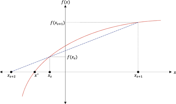

  

  Secant method

The altered algorithm is called the Modified or Quasi-Newton Method. In the following, we will state the algorithm for the case in which we do not have to solve one single non-linear equation, f(x) = 0, but a system of system of n non-linear equations in the unknowns x = [x ₁, x ₂, …, x _n]:

$$\displaystyle \begin{aligned} \left. \begin{aligned} 0 &= f^1(x_1, x_2, \dots, x_n),\\ 0 &= f^2(x_1, x_2, \dots, x_n),\\ \vdots &= \vdots \\ 0 &= f^n(x_1, x_2, \dots, x_n), \end{aligned} \right\rbrace \Longleftrightarrow {0} = {f}({x}). \end{aligned} $$

(2.60)

The equivalent to f′(x) in the multi-variable case is the Jacobian matrix J(x) of partial derivatives of f = [f ¹, f ², …, f ⁿ]′ with respect to x _i, i = 1, 2, …n. We use the notation

$$\displaystyle \begin{aligned}f^i_j := \frac{\partial f^i({x})}{\partial x_j}.\end{aligned}$$

The Jacobian is defined by:

(2.61)

Algorithm 2.2 (Modified Newton-Raphson)

This algorithm is implemented in the numerical Gauss routine FixVMN1(.) that we use in our programs.⁵³ In MATLAB, the command fsolve computes the solution to non-linear equations.

The most pressing remaining problem for the researcher who wants to apply the Newton-Rhapson algorithm and the routine FixVMN1(.) is to come up with a good initial guess that is close to the true solution. If the guess is not close enough, the sequence x _s, s = 1, 2, …, might not converge. Possible methods to find a good initial guess are as follows:

• 1. Grid search over an interval. Of course, in this case, we have to ensure that the algorithm may not have to evaluate the function at a point that results in a breakdown (e.g., 1∕0 or (−2.5)^1∕2).

• 2. Educated guess.

• 3. Genetic search.

• 4. Backstepping.

A diligent discussion of these problems is provided in Chapter 11.5 of Heer and Maußner (2009). We will also discuss this problem in the upcoming applications in this book if appropriate.

Appendix 2.3: Solving the Benchmark RBC Model

In this appendix, we compute the solution of the benchmark real business cycle (RBC) model described in Sect. 2.4. To solve it we use a linear approximation of the system of difference equations at the steady state. The algorithm is based upon the pioneering work of Blanchard and Kahn (1980) and follows the approach of King and Watson (2002).⁵⁴

Our model is described by the first-order condition of the household, (2.36), and the resource constraint (2.44). After substitution of the factor prices from (2.43) and the production function, $y_t=Z_t k_t^\alpha L_t^{1-\alpha }$, the equilibrium can be presented by the following equations in k _t, λ _t, c _t, and L _t:

$$\displaystyle \begin{aligned} \lambda_t &= \iota c_t^{\iota (1-\sigma)-1} (1-L_t)^{(1-\iota)(1-\sigma)}, \end{aligned} $$

(2.62a)

$$\displaystyle \begin{aligned} \lambda_t (1-\alpha) Z_t k_t^\alpha L_t^{-\alpha} &= (1-\iota) c_t^{\iota (1-\sigma)} (1-L_t)^{(1-\iota)(1-\sigma)-1}, \end{aligned} $$

(2.62b)

$$\displaystyle \begin{aligned} (1+n) \lambda_t&= \mathbb{E}_t \lambda_{t+1}\beta \left[1+\alpha Z_{t+1} k_{t+1}^{\alpha-1} L_{t+1}^{1-\alpha}-\delta\right], \end{aligned} $$

(2.62c)

$$\displaystyle \begin{aligned} Z_t k_t^\alpha L_t^{1-\alpha} &= c_t + (1+n) k_{t+1}- (1-\delta) k_t. \end{aligned} $$

(2.62d)

We have to distinguish four types of variables in the stochastic system of difference equations (2.62). First, we have the predetermined variables x _t. In our case, the only predetermined variable in period t is the capital stock k _t because investment i _t−1 = k _t − (1 − δ)k _t−1 was already chosen at the end of period t − 1. The second set of variables are the so-called costate variables λ _t. The number of these variables must be equal to the number of dynamic equations (those equations that contain variables from both periods t and t + 1) minus the number of predetermined variables. Therefore, we need one costate variable. In addition, the costate variables must be dynamic, i.e., these variables must appear in the system of equations with time index t + 1. In our case, the Lagrange multiplier λ _t is the costate variable. The third type of variables are control variables u _t, which are the remaining variables in the model that are either chosen by the household and/or the firm, e.g., labor supply, or that are determined by equilibrium conditions, e.g., the prices that equate demand and supply. In our case, the control variables are consumption c _t and labor L _t. Finally, the fourth type of variable is the exogenous state variable, which is the technology shock Z _t.

To solve the system of equations (2.62), we linearize it around the deterministic steady state in a first step and solve the linearized system in a second step. Therefore, we first successively linearize each of the equations in (2.62) starting with (2.62a). We take the logarithm of (2.62a):

$$\displaystyle \begin{aligned} \ln \lambda_t = \ln \iota - \left[ 1-\iota (1-\sigma)\right] \ln c_t + (1-\iota)(1-\sigma) \ln (1-L_t).\end{aligned}$$

and compute the total differential of this equation in steady state with Z _t = Z, k _t = k, c _t = c, and L _t = L:

$$\displaystyle \begin{aligned} \frac{d \lambda_t}{\lambda} = -\left[ 1-\iota (1-\sigma)\right] \frac{dc_t}{c}- (1-\iota)(1-\sigma)\frac{L}{1-L}\frac{dL_t}{L}.\end{aligned}$$

Using the notation $\hat x_t \equiv dx_t/x$ for the percentage deviation of the variable x ∈{Z, k, c, L, λ}, we obtain:

$$\displaystyle \begin{aligned} \hat \lambda_t = -\left[ 1-\iota (1-\sigma)\right] \hat c_t- (1-\iota)(1-\sigma)\frac{L}{1-L} \hat L_t.\end{aligned}$$

Similarly, we log-linearize (2.62b):

$$\displaystyle \begin{aligned} \alpha \hat k_t + \hat \lambda_t + \hat Z_t = \iota (1-\sigma) \hat c_t +\underbrace{\left[1-(1-\iota)(1-\sigma)\frac{L}{1-L} +\alpha \right]}_{\zeta} \hat L_t.\end{aligned}$$

Rearranging terms, we find

$$\displaystyle \begin{aligned} \left(\begin{array}{cc} -\left[ 1-\iota (1-\sigma)\right] & - (1-\iota)(1-\sigma)\frac{L}{1-L}\\ \iota (1-\sigma) & \zeta \end{array} \right) \left(\begin{array}{c} \hat c_t\\ \hat L_t \end{array} \right) = \left(\begin{array}{cc} 0~1\\ \alpha ~1 \end{array} \right) \left(\begin{array}{c} \hat k_t\\ \hat \lambda_t \end{array} \right)+ \left(\begin{array}{c} 0\\ 1 \end{array} \right) \hat Z_t,\end{aligned} $$

(2.63)

or, evaluated in steady state,

$$\displaystyle \begin{aligned} \underbrace{\left(\begin{array}{cc} -1.3375 & 0.2839\\ -0.3375 & 1.0725 \end{array} \right)}_{C_u} \left(\begin{array}{c} \hat c_t\\ \hat L_t \end{array} \right) = \underbrace{\left(\begin{array}{cc} 0.0000 & 1.0000\\ 0.3600 & 1.0000 \end{array} \right)}_{C_{x\lambda}} \left(\begin{array}{c} \hat k_t\\ \hat \lambda_t \end{array} \right)+ \underbrace{\left(\begin{array}{c} 0.0000\\ 1.0000 \end{array} \right)}_{C_Z} \hat Z_t. \end{aligned} $$

(2.64)

More generally, we can write (2.64) in the following form:

(2.65)

where we define the variables u _t, x _t, Λ _t, and z _tas follows:

$$\displaystyle \begin{aligned} {u}_t\equiv \left(\begin{array}{c} \hat c_t\\ \hat L_t \end{array} \right),\;\;\; {x}_t \equiv \hat k_t,\;\;\; {\varLambda}_t \equiv \hat \lambda_t,\;\;\; {z}_t \equiv \hat Z_t.\end{aligned}$$

Next we consider (2.62c), substitute r _t = αZ _t(L _t∕k _t)^1−α and differentiate totally in steady state:

$$\displaystyle \begin{aligned} d\lambda_t = \mathbb{E}_t \left[ d\lambda_{t+1} +\frac{\lambda \beta r}{1+n} \left( \frac{dZ_{t+1}}{Z} - (1-\alpha) \frac{dk_{t+1}}{k}+(1-\alpha)\frac{dL_{t+1}}{L}\right) \right] \end{aligned}$$

and, after dividing by λ:

$$\displaystyle \begin{aligned} \frac{(1-\alpha) \beta r}{1+n} \mathbb{E}_t \hat k_{t+1} - \mathbb{E}_t \hat \lambda_{t+1}+ \hat \lambda_t = \frac{(1-\alpha) \beta r}{1+n} \mathbb{E}_t \hat L_{t+1} + \frac{\beta r}{1+n} \mathbb{E}_t\hat Z_{t+1}.\end{aligned} $$

(2.66)

Finally, the resource constraint of the economy is presented by (2.62d). Taking the total differential in steady state yields

$$\displaystyle \begin{aligned} \hat Z_t + \left[ \alpha + (1-\delta) \frac{k}{y}\right] \hat k_t + (1-\alpha) \hat L_t= \frac{c}{y} \hat c_t + (1+n) \frac{k}{y} \hat k_{t+1}.\end{aligned}$$

Rearranging the last two log-linearized equations, we obtain

$$\displaystyle \begin{aligned} \begin{aligned} & \left(\begin{array}{cc} \frac{(1-\alpha) \beta r}{1+n} & -1\\ (1+n) \frac{k}{y}& 0 \end{array}\right) \mathbb{E}_t \left(\begin{array}{c} \hat k_{t+1}\\ \hat \lambda_{t+1} \end{array}\right)+ \left(\begin{array}{cc} 0& 1\\ -\left[ \alpha + (1-\delta) \frac{k}{y}\right] &0 \end{array}\right) \left(\begin{array}{c}\hat k_{t}\\ \hat \lambda_{t} \end{array}\right)\\ &= \left(\begin{array}{cc} 0 & \frac{(1-\alpha) \beta r}{1+n}\\ 0 & 0 \end{array} \right) \mathbb{E}_t \left(\begin{array}{c} \hat c_{t+1}\\ \hat L_{t+1}\end{array}\right) + \left(\begin{array}{cc} 0 & 0 \\ - \frac{c}{y} & (1-\alpha) \end{array} \right) \left(\begin{array}{c} \hat c_{t}\\ \hat L_{t}\end{array}\right) \\ & + \left(\begin{array}{c} \frac{\beta r}{1+n}\\ 0 \end{array} \right) \mathbb{E}_t \hat Z_{t+1} + \left(\begin{array}{c} 0\\ 1 \end{array} \right) \hat Z_{t}. \end{aligned} \end{aligned} $$

(2.67)

Computing the matrices of this system of equations by plugging in the parameter and equilibrium values of the model, we derive

$$\displaystyle \begin{aligned} \begin{aligned} & \underbrace{\left(\begin{array}{cc} 0.0191 &-1.0000\\ 11.96 & 0.0000 \end{array}\right)}_{D_{x\lambda}} \mathbb{E}_t \left(\begin{array}{c} \hat k_{t+1}\\ \hat c_{t+1} \end{array}\right)+ \underbrace{\left(\begin{array}{cc} 0 & 1.0000 \\ -12.0805 & 0 \end{array}\right)}_{F_{x\lambda}} \left(\begin{array}{c}\hat k_{t}\\ \hat c_{t} \end{array}\right)\\ &= \underbrace{\left(\begin{array}{cc} 0 & 0.0191\\ 0 & 0 \end{array} \right)}_{D_u} \left(\begin{array}{c}\hat c_{t+1}\\ \hat L_{t+1}\end{array}\right) + \underbrace{\left(\begin{array}{cc} 0 & 0\\ -0.7608 & 0.6400 \end{array} \right)}_{F_u} \left(\begin{array}{c}\hat c_{t}\\ \hat L_{t} \end{array}\right)+ \underbrace{\left(\begin{array}{c} 0.0298\\ 0 \end{array} \right)}_{D_z} \mathbb{E}_t \hat Z_{t+1} \\ & + \underbrace{\left(\begin{array}{c} 0\\ 1.000 \end{array} \right)}_{F_z} \hat Z_{t}. \end{aligned}\end{aligned} $$

More generally, this equation can be written as:

(2.68)

Collecting all dynamic equations characterizing our linearized stochastic system of difference equations, we derive (2.69):

(2.69a)

(2.69b)

$$\displaystyle \begin{aligned} \notag &+ D_z \mathbb{E}_t {z}_{t+1} + F_z {z}_t.\end{aligned} $$

In addition, we assume that Z _t is governed by the AR(1)-process (2.45):

$$\displaystyle \begin{aligned} \hat Z_t = \rho^Z \hat Z_{t-1} +\epsilon_t.\end{aligned} $$

To reduce the system, we assume that the first equation can be solved for the vector u _t:

(2.70)

In our case,

$$\displaystyle \begin{aligned} \left( \begin{array}{c} \hat c_t \\ \hat L_t \end{array} \right) =\left( \begin{array}{cc} 0.0764 & -0.5891\\ 0.3597 & 0.7470 \end{array} \right) \left( \begin{array}{c} \hat k_t\\ \hat \lambda_t \end{array} \right) + \left( \begin{array}{c} 0.2120\\ 0.9992 \end{array} \right) \hat Z_t. \end{aligned} $$

(2.71)

Shifting the time index one period into the future and taking expectations conditional on information as of period t yields:

(2.72)

The solutions (2.70) and (2.72) allow us to eliminate u _t and $\mathbb {E}_t{u}_{t+1}$ from (2.69b):

Assume that the matrix $D_{x\lambda }-D_u C_u^{-1}C_{x\lambda }$ is invertible. Furthermore, (2.45) implies $\mathbb {E}_t {z}_{t+1} = \rho ^Z {z}_t$. Consequently, we obtain the reduced dynamic system:

(2.73)

In our example,

(2.74)

Next, we proceed in the same way as in the derivation of our stability result in Sect. 2.2.2. In particular, we use the Schur factorization of W:

$$\displaystyle \begin{aligned}S = T^{-1} W T ,\end{aligned}$$

with

$$\displaystyle \begin{aligned} S=\left(\begin{array}{cc} 0.9695 & 0.0651\\ 0.0000 & 1.0419 \end{array}\right),\,\;\; T=\left(\begin{array}{cc} 0.8154 & 0.5789\\ -0.5789 & 0.8154 \end{array}\right). \end{aligned}$$

We can reformulate the equation in the transformed variables

(2.75)

Multiplying (2.74) by T ⁻¹, we obtain

We solve this difference equation line by line, starting with the last line. Accordingly,

$$\displaystyle \begin{aligned} \mathbb{E}_t \tilde \lambda_{t+1} = 1.0419 \tilde \lambda_t + 0.03545 \hat Z_t.\end{aligned}$$

Rearranging this equation, we obtain

$$\displaystyle \begin{aligned} \begin{aligned} \tilde \lambda_t &=\frac{1}{1.0419} \mathbb{E}_t \tilde \lambda_{t+1} \underbrace{-0.0340}_{\rho_1} \hat Z_t\\ &= \frac{1}{1.0419} \mathbb{E}_t \left( \frac{1}{1.0419} \mathbb{E}_{t+1} \tilde \lambda_{t+2} +\rho_1 \hat Z_{t+1} \right) +\rho_1 \hat Z_t\\ &=\ldots\\ &= \lim_{i\to\infty} \mathbb{E}_t \frac{1}{1.0419^i} \tilde \lambda_{t+i} + \rho_1 \left( \hat Z_t + \frac{\rho^Z}{1.0419} \hat Z_t +\ldots \right)\\ &=\frac{\rho_1}{1-\frac{\rho^Z}{1.0419}} \hat Z_t\\ &=-0.3854 \hat Z_t, \end{aligned} \end{aligned}$$

where we have used the assumptions that (1) $\mathbb {E}_t \hat Z_{t+i}=(\rho ^Z)^i \hat Z_t$ and (2) $\lim _{i\to \infty } \tilde \lambda _{t+i}<\infty$. Noticing that $\tilde \lambda _t = 0.5789 \hat k_t +0.8154 \hat \lambda _t$, we derive

$$\displaystyle \begin{aligned} \hat \lambda_t = -\frac{0.5789}{0.8154} \hat k_t -\frac{0.3854}{0.8154}\hat Z_t = -0.7099 \hat k_t -0.4727\hat Z_t.\end{aligned} $$

(2.76)

Therefore, we have derived the policy function for the marginal utility of consumption, $\hat \lambda _t$, given the values of the state variables $\hat k_t$ and $\hat Z_t$.

Next, we have to solve the first line of the difference equation

$$\displaystyle \begin{aligned} \tilde k_{t+1} = 0.9695 \tilde k_t +0.0651 \tilde \lambda_t + 0.1264 \hat Z_t.\end{aligned}$$

Substituting for $\tilde k_t$ and $\tilde \lambda _t$ from (2.75) and for $\hat \lambda _t$ from (2.76), we find that⁵⁵

$$\displaystyle \begin{aligned} \hat k_{t+1} = 0.9695 \hat k_t + 0.0870 \hat Z_t.\end{aligned} $$

(2.77)

With the help of the policy function for $\hat \lambda _t$, we can also compute the policy function for $\hat c_t$ and $\hat L_t$ from (2.71):

$$\displaystyle \begin{aligned} \left( \begin{array}{c}\hat c_t\\ \hat L_t\end{array}\right) =\left( \begin{array}{c} 0.4946\\-0.1706\end{array}\right) \hat k_t + \left( \begin{array}{c}0.4908\\0.6457\end{array}\right) \hat Z_t.\end{aligned}$$

Similarly, we can compute the policy function for output, wages, and the interest rate with the help of $\hat L_t$ from

$$\displaystyle \begin{aligned} \begin{aligned} \hat y_t & =\hat Z_t + \alpha \hat k_t + (1-\alpha) \hat L_t, \\ \hat r_t & =\hat Z_t -\alpha \hat k_t + (1-\alpha) \hat L_t,\\ \hat w_t & = \hat Z_t +\alpha \hat k_t - (1-\alpha) \hat L_t. \end{aligned} \end{aligned}$$

Appendix 2.4: Data Sources

Most data are taken from the FRED database of the Federal Reserve Bank of St. Louis at https://research.stlouisfed.org/fred2/, where you can download many US macroeconomic time series (Accessed on 28 October 2015). The time series that we use in this chapter are also attached as a separate ASCII file “Fred_Data.txt” to my Matlab/Gauss programs.

• Output Gross Domestic Product. Bureau of Economic Analysis (BEA), retrieved from FRED, Federal Reserve Bank of St. Louis. Series ID: GDPA.

• Consumption Real Personal Consumption Expenditures, Billions of Chained 2009 Dollars, Quarterly, Seasonally Adjusted Annual Rate. Series ID: PCECC96.

• Investment Private Nonresidential Fixed Investment. BEA, retrieved from FRED, Federal Reserve Bank of St. Louis. Series ID: PNFIA.

• Labor Supply Nonfarm Business Sector: Hours of All Persons. US. Bureau of Labor Statistics, retrieved from FRED, Federal Reserve Bank of St. Louis. Series ID: HOANBS.

• Wages Nonfarm Business Sector—Compensation Per Hour. BLS, retrieved from FRED, Federal Reserve Bank of St. Louis. Series ID: COMPNFB.

• Nominal Interest Rate for the Risk-free Rate 3-Month Treasury Bill: Secondary Market Rate, Percent, Quarterly, Not Seasonally Adjusted. Series ID: TB3MS.

• Nominal Equity Return Standard & Poor’s 500 Total Return, Yield, Percent, Quarterly, Not Seasonally Adjusted, own calculation.

• Inflation Rate Personal Consumption Expenditures: Chain-type Price Index Less Food and Energy, Index 2009 = 100, Quarterly, Seasonally Adjusted, retrieved from FRED, Federal Reserve Bank of St. Louis. Series ID: JCXFE.

Problems

2.1

Compute the dynamics for the centralized deterministic Ramsey model with labor supply as presented in Fig. 2.9 for the case of a CES production function (2.6). Use the value σ _p = 3∕4 for the production substitution elasticity as in Heer and Schubert (2012). For all other parameters, use the values provided in Sect. 2.2.

2.2

Compute the Jacobian (2.16) at the steady state k _t = k, x _t = k.

2.3

Consider the market economy described in Sect. 2.3. Assume that the government has to finance exogenous expenditures G _t that do not affect utility or production (in Chap. 4, we will modify this assumption). Consider two cases:

• 1. Government expenditures are financed by a lump-sum tax T _t such that each household pays T _t∕N _t.

• 2. Government expenditures are financed by a tax on wage income such that the individual household pays τ _t w _t L _t in taxes.

Is the allocation in the economy in both cases Pareto-optimal?

2.4

Consider the market economy described in Sect. 2.3. Assume that the initial capital stock per capita amounts to 50% of its steady state value.

• 1. Compute the transition dynamics to the steady state. Assume that the transition is completed after 50 periods. How does the savings rate behave during the transition? Contrast your finding in the Ramsey model with the Solow model where the savings rate is constant.

• 2. Introduce capital adjustment costs into the Ramsey model. For this reason, assume that the household faces the following costs to increase its capital stock:

  $$\displaystyle \begin{aligned} k_{t+1} = (1-\delta) k_t + \varPhi \left( \frac{i_t}{k_t}\right),\end{aligned}$$

  where i _t denotes investment and Φ(.) is a concave function that takes the following form:

  $$\displaystyle \begin{aligned} \varPhi \left( \frac{i_t}{k_t}\right) = \frac{a_1}{1-\zeta} \left( \frac{i_t}{k_t}\right)^{1-\zeta} + a_2.\end{aligned}$$

  Calibrate the parameter of the adjustment cost function Φ(.) as follows: ζ = 1∕0.23 is taken from Jermann (1998). Assume that adjustment costs play no role in steady state, meaning that i = δk, and that the multiplier of the adjustment cost constraint in the Lagrangian,

  $$\displaystyle \begin{aligned}\begin{aligned} \mathscr{L}&= \sum_{t=0}^\infty \beta^t \left\{ u(c_t,L_t) + \lambda_t \left[ w_t L_t + r_t k_t - c_t -i_t \right]\right.\\ &\left.+ q_t \left[ k_{t+1}-(1-\delta) k_t - \varPhi \left( \frac{i_t}{k_t}\right)\right]\right\} \end{aligned}\end{aligned}$$

  is equal to one in steady state, q = 1, implying

  $$\displaystyle \begin{aligned} a_1 = \delta^\zeta,\end{aligned}$$

  and

  $$\displaystyle \begin{aligned} a_2 = \frac{-\zeta}{1-\zeta} \delta.\end{aligned}$$

  How do capital adjustment costs affect the savings rate during the transition?

• 3. Compute the impulse responses and the time series statistics for the RBC model with capital adjustment costs.

2.5

Two-Sector Model (follows Heer, Maußner, and Süssmuth 2018 ) Consider a two-sector economy in which a consumption and an investment good are produced in separate production sectors. The consumption goods sector (subscript C) employs the technology

$$\displaystyle \begin{aligned} C_t = Z_{Ct} L_{Ct}^{1-\alpha}K_{Ct}^\alpha, \quad \alpha\in (0,1), \end{aligned}$$

where L _Ct and K _Ct denote labor and capital employed in this sector. Z _Ct denotes the total factor productivity (TFP). We assume that the log of Z _Ct follows a random walk with drift parameter a _C and (possibly) autocorrelated innovations 𝜖 _Ct:

$$\displaystyle \begin{aligned} \begin{aligned} \ln Z_{Ct} &= \ln Z_{Ct-1} + a_C + \epsilon_{Ct},\\ \epsilon_{Ct} & = \rho^{C}\epsilon_{Ct-1}+\eta_{Ct},\quad \eta_{Ct} \text{ iid } \mathscr{N}(0,\sigma^C). \end{aligned} \end{aligned}$$

The investment goods sector (subscript I) uses the production technology

$$\displaystyle \begin{aligned} I_t = Z_{It} L_{It}^{1-\alpha}K_{It}^\alpha, \end{aligned}$$

so that I _t is the amount of investment goods in period t which sell at the relative price p _t. The process for total factor productivity in the investment sector is also difference stationary, yet with a different drift rate a _I:

$$\displaystyle \begin{aligned} \begin{aligned} \ln Z_{It} &= \ln Z_{It-1} + a_I + \epsilon_{It},\\ \epsilon_{It} & = \rho^{I}\epsilon_{It-1}+\eta_{It},\quad \eta_{It} \text{ iid } \mathscr{N}(0,\sigma^I). \end{aligned} \end{aligned}$$

The economy’s output in units of the consumption good is equal to

$$\displaystyle \begin{aligned} Y_t = C_t + p_t I_t. \end{aligned}$$

Total labor and capital in the economy equal

$$\displaystyle \begin{aligned} \begin{aligned} L_t &= L_{Ct} + L_{It},\\ K_t &= K_{Ct} + K_{It}. \end{aligned} \end{aligned}$$

The firms in the two sector maximize profits

$$\displaystyle \begin{aligned} \begin{aligned} \varPi^C_t&=C_{t} - w_{Ct+s}L_{Ct} - p_{t} I_{Ct},\\ {} \varPi^I_t&=p_{t}I_{t} - w_{It}L_{It} - p_{t} I_{It}. \end{aligned} \end{aligned}$$

A representative household supplies labor L _Ct to the consumption goods sector and L _It to the investment goods sector. The respective wage rates are w _Ct and w _It and are equal to each other in equilibrium. The household maximizes intertemporal utility

$$\displaystyle \begin{aligned} \max \mathbb{E}_t \sum_{s=0}^\infty \beta^s u\left(C_{t+s}, L_{t+s}\right), \end{aligned}$$

where its instantaneous utility function u depends on consumption C _t and labor L _t:

$$\displaystyle \begin{aligned} u(C_t, N_t) = \ln (C_t) - \frac{\nu_0}{1+\nu_1}L_t^{1+1/\nu_1},\quad \nu_0, \nu_1 > 0. \end{aligned}$$

The household also owns the capital stock which is subject to adjustment costs:

$$\displaystyle \begin{aligned} K_{Xt+1} = \varPhi_X(I_{Xt}/K_{Xt})K_{Xt}+ (1-\delta)K_{Xt},\quad \delta\in (0,1],\quad X\in\{C,I\}, \end{aligned}$$

where δ denotes the rate of capital depreciation and the adjustment cost functions Φ _X, X ∈{C, I}, have the same functional forms as the one specified in Problem 2.4 above.

• 1. Derive the equilibrium conditions of the model.

• 2. Reformulate the equilibrium equations in stationary variables. Show that, in the long-run, the relative price of the two goods p _t is driven by the different rates of technological progress.

• 3. Compute the model and its impulse responses to a productivity shock in the two sectors. Use the calibration of Heer, Maußner, and Süssmuth (2018): β = 0.994, ν ₁ = 0.3, α = 0.36, δ = 0.021, ζ _C = 6.0, ζ _I = 2.0, a _C = 0.00054, a _I = 0.0077, ρ ^C = 0, ρ ^I = 0.28, σ ^C = 0.0070, σ ^I = 0.0084, and the steady state value of labor L = 0.33 for the calibration of ν ₀. How do the responses differ between the productivity shocks to the consumption and investment goods sectors?

2.6

For the two-period model in Appendix 2.1, show that the optimal consumption in period 1, c ₁, is given by:

$$\displaystyle \begin{aligned} c_1 = \frac{y_1 + \frac{y_2}{1+r} } { 1+ \beta^{1/\sigma} \left[1+r \right]^{1/\sigma-1} }.\end{aligned} $$

(2.78)

For y ₂ = 0, it follows immediately that $\frac {\partial c_1}{\partial r}>0$ if and only if 1∕σ > 1. Recompute the values in the Tables 2.2 and 2.3 in Appendix 2.1 with the help of Gauss (use the proc() command to compute the value of the function (2.78)) or MATLAB.

References

Attanasio, O., & Low, H. (2004). Estimating Euler equations. Review of Economic Dynamics, 7, 406–435.
Auerbach, A. J., & Kotlikoff, L. (1987). Dynamic fiscal policy. New York: Cambridge University Press.
Azariadis, C. (1993). Intertemporal macroeconomics. Oxford: Blackwell.
Basu, S., Fernald, J. G., & Kimball, M. S. (2006). Are technology improvements contractionary?. American Economic Review, 96, 1418–1448.
Baxter, M., & King, R. G. (1999). Measuring business cycles: Approximate band-pass filters for economic time series. Review of Economics and Statistics, 81(4), 575–593.
Beaudry, P., & Portier, F. (2004). An exploration into Pigou’s theory of cycles. Journal of Monetary Economics, 51(6), 1183–1216.
Beaudry, P., & Portier, F. (2006). Stock prices, news, and economic fluctuations. American Economic Review, 596(4), 1293–1307.
Blanchard, O. J., & Kahn, C. M. (1980). The solution of linear difference models under rational expectations. Econometrica, 48, 1305–1311.
Cass, D. (1965). Optimum growth in an aggregative model of capital accumulation. Review of Economic Studies, 32, 233–240.
Cogley, T., & Nasan, J. M. (1995). Output dynamics in real-business-cycle models. American Economic Review, 85, 492–511.
Cooley, T. F. (1995). Frontiers of business cycle research. Princeton: Princeton University Press.
Cooley, T. F., & Prescott, E. C. (1995). Economic growth and business cycles. In T. F. Cooley (Ed.), Frontiers of business cycle research (pp. 1–64). Princeton: Princeton University Press.
deJong, D. N., & Dave, C. (2011). Structual macroeconometrics (2nd ed.). Princeton: Princeton University Press.
Galí, J. (1999). Technology, employment, and the business cycle: Do technology shocks explain aggregate fluctuations?. American Economic Review, 89, 249–271.
Gandolfo, G. (2009). Economic dynamics. Berlin/Heidelberg: Springer.
Heer, B., & Maußner, A. (2009). Dynamic general equilibrium modeling: Computational methods and applications (2nd ed.). Heidelberg: Springer.
Heer, B., Maußner, A., & Süssmuth, B. (2018). Cyclical asset returns in the consumption and investment goods sector. Review of Economic Dynamics, 28, 51–70.
Heer, B., & Schubert, S. F. (2012). Unemployment and debt dynamics in a highly indebted small open economy. Journal of International Money and Finance, 31, 1392–1413.
Hodrick, R. J., & Prescott, E. C. (1997). Postwar US business cycles: An empirical investigation. Journal of Money, Credit, and Banking, 29, 1–16.
Jermann, U. J. (1998). Asset pricing in production economies. Journal of Monetary Economics, 41, 257–275.
Judd, K. L. (1998). Numerical methods in economics. Cambridge: MIT Press.
King, R. G., & Watson, M. W. (2002). System reduction and solution algorithms for singular difference systems under rational expectations. Computational Economics, 20, 57–86.
Koopmans, T. C. (1965). On the concept of optimal economic growth. In The econometric approach to development planning (pp. 225–287). Amsterdam: North-Holland.
Kydland, F. E., & Prescott, E. C. (1982). Time to build and agregate fluctuations. Econometrica, 50, 1345–1370.
Long, J. B., & Plosser, C. I. (1983). Real business cycles. Journal of Political Economy, 91, 39–69.
McCandless, G. (2008). The ABCs of RBCs. Cambridge: Harvard University Press.
McGrattan, E. R., & Prescott, E. C. (2014). A reassessment of real business cycle theory. American Economic Review, 104, 177–182.
Mehra, R., & Prescott, E. C. (1985). The equity premium: a puzzle. Journal of Monetary Economics, 15, 145–161.
Miranda, M. J., & Fackler, P. L. (2002). Applied computational economics and finance. Cambridge: MIT Press.
Muth, J. F. (1961). Rational expectations and the theory of price movements. Econometrica, 29, 315–335.
Prescott, E. C. (1986). Theory ahead of business-cycle measurement. Carnegie-Rochester Conference on Public Policy, 24, 11–44.
Ramsey, F. (1928). A mathematical theory of saving. Economic Journal, 38, 543–559.
Ravn, M. O., & Uhlig, H. (2001). On adjusting the HP-filter for the frequency of observations (CEPR Discussion Paper, 2858).
Author information
Authors and Affiliations