
Abstract
Categorical studies of recursive data structures and their associated reasoning principles have mostly focused on two extremes: initial algebras and induction, and final coalgebras and coinduction. In this paper we study their in-betweens. We formalize notions of alternating fixed points of functors using constructions that are similar to that of free monads. We find their use in categorical modeling of accepting run trees under the Büchi and parity acceptance condition. This modeling abstracts away from states of an automaton; it can thus be thought of as the “behaviors” of systems with the Büchi or parity conditions, in a way that follows the tradition of coalgebraic modeling of system behaviors.
You have full access to this open access chapter, Download conference paper PDF
1 Introduction
Büchi Automata. The Büchi condition is a common acceptance condition for automata for infinite words. Let \(x_{i}\in X\) be a state of an automaton \(\mathcal {A}\) and \(a_{i}\in \mathsf {A}\) be a character, for each \(i\in \omega \). An infinite run \(x_{0}\!\xrightarrow {a_{0}}\!x_{1}\!\xrightarrow {a_{1}}\!\cdots \) satisfies the Büchi condition if \(x_{i}\) is an accepting state (usually denoted by  ) for infinitely many i. An example of a Büchi automaton is shown on the right. The word \((ba)^{\omega }\) is accepted, while \(ba^{\omega }\) is not. A function that assigns each \(x\in X\) the set of accepted words from x is called the trace semantics of the Büchi automaton.

Categorical Modeling. The main goal of this paper is to give a categorical characterization of such runs under the Büchi condition. This is in the line of the established field of categorical studies of finite and infinite datatypes: it is well-known that finite trees form an initial algebra, and infinite trees form a final coalgebra; and finite/infinite words constitute a special case. These categorical characterizations offer powerful reasoning principles of (co)induction for both definition and proof. While the principles are categorically simple ones corresponding to universality of initial/final objects, they have proved powerful and useful in many different branches of computer science, such as functional programming and process theory. See the diagram on the right above illustrating coinduction: given a functor F, its final coalgebra  has a unique homomorphism to it from an arbitrary F-coalgebra \(d:Y\rightarrow FY\). In many examples, a final coalgebra is described as a set of “infinite F-trees.”
Extension of such (co)algebraic characterizations of data structures to the Büchi condition is not straightforward, however. A major reason is the non-local character of the Büchi condition: its satisfaction cannot be reduced to a local, one-step property of the run. For example, one possible attempt of capturing the Büchi condition is as a suitable subobject of the set \(\mathrm {Run}(X)=(\mathsf {A}\times X)^{\omega }\) of all runs (including nonaccepting ones). The latter set admits clean categorical characterization as a final coalgebra  for the functor \(F=(\mathsf {A}\times X)\times \underline{~}\,\). Specifying its subset according to the Büchi condition seems hard if we insist on the coalgebraic language which is centered around the local notion of transition represented by a coalgebra structure morphism \(c:X\rightarrow FX\).
There have been some research efforts in this direction, namely the categorical characterization of the Büchi condition. In [5] the authors insisted on finality and characterize languages of Muller automata (a generalization of Büchi automata) by a final coalgebra in \(\mathbf {Sets}^2\). Their characterization however relies on the lasso characterization of the Büchi condition that works only in the setting of finite state spaces. In [21] we presented an alternative characterization that covers infinite state spaces and automata with probabilistic branching. The key idea was the departure from coinduction, that is, reasoning that relies on the universal property of greatest fixed points. Note that a final coalgebra  is a “categorical greatest fixed point” for a functor F.
Our framework in [21] was built on top of the so-called Kleisli approach to trace semantics of coalgebras [10,11,12, 16]. There a system is a coalgebra in a Kleisli category  , where T represents the kind of branching the system exhibits (nondeterminism, probability, etc.). A crucial fact in this approach is that homsets of the category
  come with a natural order structure. Specifically, in [21], we characterized trace semantics under the Büchi condition as in the diagrams (1) belowFootnote 1, where (i) \(X_1\) (resp. \(X_2\)) is the set of nonaccepting (resp. accepting) states of the Büchi automaton (i.e. \(X=X_1+X_2\)), and (ii) the two diagrams form a hierarchical equation system (HES), that is roughly a planar representation of nested and alternating fixed points. In the HES, we first calculate the least fixed point for the left diagram, and then calculate the greatest fixed point for the right diagram with \(u_1\) replaced by the obtained least fixed point. Note that the order of calculating fixed points matters.

Contributions: Decorated Trace Semantics by Categorical Datatypes. In this paper we introduce an alternative categorical characterization to the one in [21] for the Büchi conditions, where we do not need alternating fixed points in homsets. This is made possible by suitably refining the value domain, from a final coalgebra to a novel categorical datatypes \(F^{+{\oplus }}0\) and \(F^{+}(F^{+{\oplus }}0)\) that have the Büchi condition built in them. Diagrammatically the characterization looks as in (2) below. Note that we ask for the greatest fixed point in both squares.

The functors \(F^{+}\) and \(F^{+{\oplus }}\) used in the datatypes are obtained by applying two operations \((\underline{~}\,)^+\) and \((\underline{~}\,)^{\oplus }\) to a functor F. For an endofunctor G on a category \(\mathbb {C}\) with enough initial algebras, \(G^+ X\) is given by the carrier object of a (choice of) an initial \(G(\underline{~}\,+X)\)-algebra for each \(X\in \mathbb {C}\). The universality of initial algebras allows one to define \(G^+f:G^+X\rightarrow G^+Y\) for each \(f:X\rightarrow Y\) and extend \(G^+\) to a functor \(G^+:\mathbb {C}\rightarrow \mathbb {C}\). This definition is much similar to that of a free monad \(G^*\), where \(G^*X\) is the carrier object of an initial \(G(\underline{~}\,)+X\)-algebra for \(X\in \mathbb {C}\). The operation \((\underline{~}\,)^{\oplus }\) is defined similarly: for \(G:\mathbb {C}\rightarrow \mathbb {C}\) and \(X\in \mathbb {C}\), \(G^{\oplus }X\) is given by the carrier object of a final \(G(\underline{~}\,+X)\)-coalgebra. This construction resembles to that of free completely iterative algebras [14].
The constructions of \(F^{+}(F^{+{\oplus }}0)\) and \(F^{+{\oplus }}0\) has a clear intuitive meaning. For the specific example of \(\mathsf {A}\)-labeled nondeterministic Büchi automata, \(T=\mathcal {P}\), \(F=\mathsf {A}\times (\underline{~}\,)\), \(F^{+}(F^{+{\oplus }}0) \cong F^{+{\oplus }}0\cong (\mathsf {A}^+)^\omega \). Hence an element in \(F^{+}(F^{+{\oplus }}0)\) or \(F^{+{\oplus }}0\) is identified with an infinite sequence of finite words. We understand it as an infinite word “decorated” with information about how accepting states are visited, by considering that an accepting state is visited at each splitting between finite words. For example, we regard \((a_0a_1)(a_2a_3a_4)(a_5a_6)(a_7)\ldots \in (\mathsf {A}^+)^\omega \cong F^{+{\oplus }}0\) as an infinite word decorated as follows.

An element in \(F^{+}(F^{+{\oplus }}0)\) is similarly understood, except that the initial state is regarded as a nonaccepting state. We note that by its definition, the resulting “decorated” word always satisfies the Büchi condition.
Thus the arrows  and
and  in (2) are regarded as a kind of trace semantics that assigns each state \(x\in X\) the set of infinite words accepted from x “decorated” with information about the corresponding accepting run. Hence we shall call \(v_1\) and \(v_2\) a decorated trace semantics for the coalgebra c. The generality of the category theory allows us to define decorated trace semantics for systems with other transition or branching types, e.g. Büchi tree automata or probabilistic Büchi automata.
In this paper, we also show the relationship between decorated trace semantics and (ordinary) trace semantics for Büchi automata. For the concrete case of Büchi automata sketched above, there exists a canonical function \((\mathsf {A}^+)^\omega \rightarrow \mathsf {A}^\omega \) that flattens a sequence and hence removes the “decorations”. It is easy to see that if we thus remove decorations of a decorated trace semantics then we obtain an ordinary trace semantics. We shall prove its categorical counterpart.
In fact, the framework in [21] also covered the parity condition, which generalizes the Büchi condition. A parity automaton is equipped with a function \(\varOmega :X\rightarrow [1,2n]\) that assigns a natural number called a priority to each state \(x\in X\). Our new framework developed in the current paper also covers parity automata. In order to obtain the value domain for parity automata, we repeatedly apply \((\underline{~}\,)^+\) and \((\underline{~}\,)^{\oplus }\) to F like \(F^{+{\oplus }\cdots +{\oplus }}0\).
Compared to the existing characterization shown in (1), one of the characteristics of our new characterization as shown in (2) is that information about accepting states is more explicitly captured in decorated trace semantics, as in (3). This characteristics would be useful in categorically characterizing notions about Büchi or parity automata. For example, we could use it for categorically characterizing (bi)simulation notions for Büchi automata, e.g. delayed simulation [8], a simulation notion known to be appropriate for state space reduction.
To summarize, our contributions in this paper are as follows:
-
We introduce a new categorical data type \(F^{+{\oplus }}0\), an alternating fixed point of a functor, for characterizing the Büchi acceptance condition.
-
Using the data type, we introduce a categorical decorated trace semantics, simply as a greatest fixed point.
-
We show the categorical relationship with ordinary trace semantics in [21].
-
We instantiate the framework to several types of concrete systems.
-
We extend the framework to the parity condition (in the appendix).
Related Work. As we have mentioned, a categorical characterization of Büchi and parity conditions is also found in [5], but adaptation to infinite-state or probabilistic systems seems to be difficult in their framework. There also exist notions which are fairly captured by their characterization but seem difficult to capture in the frameworks in [21] and this paper, such as bisimilarity.
The notion of alternating fixed point of functors is also used in [2, 9]. In [9] the authors characterize the set of continuous functions from \(A^\omega \) to \(B^\omega \) as an alternating fixed point \(\nu X.\, \mu Y.\, (B\times X)+Y^A\) of a functor. Although the data type and the one used in the current paper are different and incomparable, the intuition behind them is very similar, because the former comes with a Büchi-like flavor: if \(f(a_0a_1\ldots )=b_0b_1\ldots \) then each \(b_i\) should be determined by a finite prefix of \(a_0a_1\ldots \), and therefore f is regarded as an infinite sequence of such assignments. In [2, Sect. 7] a sufficient condition for the existence of such an alternating fixed point is discussed.
Organization. Section 2 gives preliminaries. In Sect. 3 we introduce a categorical data type for decorated trace semantics as an alternating fixed point of functors. In Sect. 4 we define a categorical decorated trace semantics, and show a relationship with ordinary categorical trace semantics in [21]. In Sect. 5 we apply the framework to nondeterministic Büchi tree automata. In Sect. 6, we briefly discuss systems with other branching types. In Sect. 7, we conclude and give future work.
All the discussions in this paper also apply to the parity condition. However, for the sake of simplicity and limited space, we mainly focus on the Büchi condition throughout the paper, and defer discussions about the parity condition to the appendix, that is found in the extended version [20] of this paper. We omit a proof if an analogous statement is proved for the parity condition in the appendix. Some other proofs and discussions are also deferred to the appendix.
2 Preliminaries
2.1 Notations
For \(m,n\in \mathbb {N}\), [m, n] denotes the set \(\{i\in \mathbb {N}\mid m\le i\le n\}\). We write \(\pi _i:\prod _{i} X_i\rightarrow X_i\) and \(\kappa _i:X_i\rightarrow \coprod _{i}X_i\) for the canonical projection and injection respectively. For a set A, \(A^*\) (resp. \(A^\omega \)) denotes the set of finite (resp. infinite) sequences over A, \(A^\infty \) denotes \(A^*\cup A^\omega \), and \(A^+\) denotes \(A^*\setminus \{\langle \rangle \}\). We write \(\langle \rangle \) for the empty sequence. For a monotone function \(f:(X,\sqsubseteq )\rightarrow (X,\sqsubseteq )\), \(\mu f\) (resp. \(\nu f\)) denotes its least (resp. greatest) fixed point (if it exists). We write \(\mathbf {Sets}\) for the category of sets and functions, and \(\mathbf {Meas}\) for the category of measurable sets and measurable functions. For \(f:X\rightarrow Y\) and \(A\subseteq Y\), \(f^{-1}(A)\) denotes \(\{x\in X\mid f(x)\in A\}\).
2.2 Fixed Point and Hierarchical Equation System
In this section we review the notion of hierarchical equation system (HES) [3, 6]. It is a kind of a representation of an alternating fixed point.
Definition 2.1
(HES). A hierarchical equation system (HES for short) is a system of equations of the following form.
Here for each \(i\in [1,m]\), \((L_i,\le _i)\) is a complete lattice, \(u_i\) is a variable that ranges over \(L_i\), \(\eta _i\in \{\mu ,\nu \}\) and \(f_i:L_1\times \dots \times L_m\rightarrow L_i\) is a monotone function.
Definition 2.2
(Solution). Let E be an HES as in Definition 2.1. For each \(i\in [1,m]\) and \(j\in [1,i]\) we inductively define \(f_i^\ddagger :L_i\times \cdots \times L_m\rightarrow L_i\) and \(l^{(i)}_{j}:L_{i+1}\times \cdots \times L_m\rightarrow L_j\) as follows (no need to distinguish the base case from the step case):
-
\(f_i^\ddagger (u_i,\ldots ,u_m):=f_i(l^{(i-1)}_{1}(u_i,\ldots ,u_m), \ldots ,l^{(i-1)}_{i-1}(u_i,\ldots ,u_m),u_i,\ldots ,u_m)\); and
-
\(l^{(i)}_{i}(u_{i+1},\ldots ,u_m)\,{:=}\,\eta f_i^\ddagger (\underline{~}\,,u_{i+1},\ldots ,u_m)\) where \(\eta =\mu \) if i is odd and \(\eta =\nu \) if i is even. For \(j\,{<}\,i\), \(l^{(i)}_{j}(u_{i+1},\ldots ,u_m)\,{:=}\,l^{(i-1)}_{j}(l^{(i)}_{i}(u_{i+1},\ldots ,u_m),u_{i+1},\ldots ,u_m)\). If such a least or greatest fixed point does not exist, then it is undefined.
We call \((l^{(i)}_{1},\ldots ,l^{(i)}_{i})\) the i-th intermediate solution. The solution of the HES E is a family \((u^\mathrm {sol}_1,\ldots ,u^\mathrm {sol}_m)\in L_1\times \cdots \times L_m\) defined by \(u^\mathrm {sol}_i:=l^{(m)}_{i}(*)\) for each i.
2.3 Categorical Finite and Infinitary Trace Semantics
We review [11, 12, 16, 18] and see how finite and infinitary traces of transition systems are characterized categorically. We assume that the readers are familiar with basic theories of categories and coalgebras. See e.g. [4, 13] for details.
We model a system as a (T, F)-system, a coalgebra \(c:X\rightarrow TFX\) where T is a monad representing the branching type and F is an endofunctor representing the transition type of the system. Here are some examples of T and F:
Definition 2.3
(\(\mathcal {P}\), \(\mathcal {D}\), \(\mathcal {L}\) and \(\mathcal {G}\)). The powerset monad is a monad \(\mathcal {P}=(\mathcal {P},\eta ^{\mathcal {P}},\mu ^{\mathcal {P}})\) on \(\mathbf {Sets}\) where  , \(\mathcal {P}f(A):=\{f(x)\mid x\in A\}\), \(\eta ^{\mathcal {P}}_X(x):=\{x\}\) and \(\mu ^{\mathcal {P}}_X(\varGamma ):=\bigcup _{A\in \varGamma }A\). The subdistribution monad is a monad \(\mathcal {D}=(\mathcal {D},\eta ^{\mathcal {D}},\mu ^{\mathcal {D}})\) on \(\mathbf {Sets}\) where \(\mathcal {D}X:=\{\delta :X\rightarrow [0,1]\mid |\{x\mid \delta (x)>0\}| \text {is countable, and }\sum _{x}\delta (x)\le 1\}\), \(\mathcal {D}f(\delta )(y):=\sum _{x\in f^{-1}(\{y\})}\delta (x)\), \(\eta ^{\mathcal {D}}_X(x)(x')\) is 1 if \(x=x'\) and 0 otherwise, and \(\mu ^{\mathcal {D}}_X(\varPhi )(x):=\sum _{\delta \in \mathcal {D}X}\varPhi (\delta )\cdot \delta (x)\). The lift monad is a monad \(\mathcal {L}=(\mathcal {L},\eta ^{\mathcal {L}},\mu ^{\mathcal {L}})\) on \(\mathbf {Sets}\) where \(\mathcal {L}X:=\{\bot \}+X\), \(\mathcal {L}f(a)\) is f(a) if \(a\in X\) and \(\bot \) if \(a=\bot \), \(\eta ^{\mathcal {L}}_X(x):=x\) and \(\mu ^{\mathcal {L}}_X(a):=a\) if \(a\in X\) and \(\bot \) if \(a=\bot \). The sub-Giry monad is a monad \(\mathcal {G}=(\mathcal {G},\eta ^{\mathcal {G}},\mu ^{\mathcal {G}})\) on \(\mathbf {Meas}\) where \(\mathcal {G}(X,\mathfrak {F}_X)\) is carried by the set of probability measures over \((X,\mathfrak {F}_X)\), \(\mathcal {G}f(\varphi )(A):=\varphi (f^{-1}(A))\), \(\eta ^{\mathcal {G}}_X(x)(A)\) is 1 if \(x\in A\) and 0 otherwise, and \(\mu ^{\mathcal {G}}_X(\varXi )(A):=\int _{\delta \in \mathcal {G}X}\delta (A)d\varXi \).
Definition 2.4
(Polynomial Functors). A polynomial functor F on \(\mathbf {Sets}\) is defined by the following BNF notation: \(F::=\mathrm {id}\mid A\mid F\times F\mid \coprod _{i\in I}F\) where \(A\in \mathbf {Sets}\) and I is countable. A (standard Borel) polynomial functor F on \(\mathbf {Meas}\) is defined by the following BNF notation: \(F::=\mathrm {id}\mid A\mid F\times F\mid \coprod _{i\in I}F\) where \(A\in \mathbf {Meas}\), I is countable, and the \(\sigma \)-algebras over products and coproducts are given in the standard manner (see e.g. [18, Definition 2.2]).
A carrier of an initial F-algebra models a domain of finite traces [11] while that of a final F-coalgebra models a domain of infinitary traces [12]. For example, as we have seen in Sect. 1, for \(F=\{\checkmark \}+\mathsf {A}\times (\underline{~}\,)\) on \(\mathbf {Sets}\), the carrier set of the final F-coalgebra is \(\mathsf {A}^\infty \) while that of the initial F-algebra is \(\mathsf {A}^*\). The situation is similar for a polynomial functor \(F=(\{\checkmark \},\mathcal {P}\{\checkmark \})+(\mathsf {A},\mathcal {P}\mathsf {A})\times (\underline{~}\,)\) on \(\mathbf {Meas}\). The carrier of an initial algebra is \((\mathsf {A}^*,\mathcal {P}\mathsf {A}^*)\), and that of a final coalgebra is \((\mathsf {A}^\infty ,\mathfrak {F}_{\mathsf {A}^\infty })\) where \(\mathfrak {F}_{\mathsf {A}^\omega }\) is the standard \(\sigma \)-algebra generated by the cylinder set.
In general, for a certain class of functors, an initial algebra and a final coalgebra are obtained by the following well-known construction.
Theorem 2.5
([1])
-
1.
Let \((A,(\pi _i:F^i0\rightarrow A)_{i\in \omega })\) be a colimit of an \(\omega \)-chain
 . If F preserves the colimit, then the unique mediating arrow \(\iota :FA\rightarrow A\) from the colimit \((FA,(F\pi _i:F^{i+1}0\rightarrow FA)_{i\in \omega })\) to a cocone \((A,(\pi '_i:F^i0\rightarrow A)_{i\in \omega })\) where \(\pi '_i=\pi _{i+1}\) is an initial F-algebra.
 -
2.
Let \((Z,(\pi _i:A\rightarrow F^i1)_{i\in \omega })\) be a limit of an \(\omega ^\mathrm {op}\)-chain \(1\xleftarrow {!}F1\xleftarrow {F!}F^21\xleftarrow {F^2!}\dots \). If F preserves the limit, then the unique mediating arrow \(\zeta :Z\rightarrow FZ\) from a cone \((Z,(\pi '_i:A\rightarrow F^i1)_{i\in \omega })\) where \(\pi '_i=\pi _{i+1}\) to the limit \((FZ,(F\pi _i:FZ\rightarrow F^{i+1}1)_{i\in \omega })\) is a final F-coalgebra.
 . If F preserves the colimit, then the unique mediating arrow
 \(\square \)
We next quickly review notions about the Kleisli category  .
.
Definition 2.6
( , J, Uand \(\overline{F}\)). Let \(T=(T,\eta ,\mu )\) be a monad on \(\mathbb {C}\). The Kleisli category
  is given by
  and
and  for
for  . An arrow
  is called a Kleisli arrow, and we write
  for distinction. Composition of arrows
  and
and  is defined by \(\mu _Z\circ Tg\circ f\), and denoted by \(g\odot f\) for distinction. The lifting functor
  is defined by: \(JX:= X\) and \(J(f):=\eta _Y\circ f\) for \(f:X\rightarrow Y\). The forgetful functor
  is defined by: \(UX:=TX\) and \(U(g):=\mu _Y\circ Tg\) for
  . A functor
  is called a lifting of \(F:\mathbb {C}\rightarrow \mathbb {C}\) if \(\overline{F}J=JF\).
Example 2.7
Let \(T=\mathcal {P}\) and \(F=\sum _{n=0}^{\omega }\varSigma _n\times (\underline{~}\,)^n:\mathbf {Sets}\rightarrow \mathbf {Sets}\). A lifting \(\overline{F}\) over  is given by \(\overline{F}X=FX\) for \(X\in \mathbf {Sets}\) and \(\overline{F}f(\sigma ,x_0,\ldots ,x_{n-1})=\{(\sigma ,y_0,\ldots ,y_{n-1})\mid \forall i.\, y_i\in f(x_i)\}\) for
  , \(\sigma \in \varSigma _n\) and \(x_0,\ldots ,x_{n-1}\in X\). (see e.g. [11]).
It is well-known that there is a bijective correspondence between a lifting \(\overline{F}\) and a distributive law, a natural transformation \(\lambda :FT\Rightarrow TF\) satisfying some axioms [15]. See Sect. D of the extended version [20] for the details.
In the rest of this section, let F be an endofunctor and T be a monad on a category \(\mathbb {C}\), and assume that a lifting  is given.
In [11], a finite trace semantics of a transition system was characterized as the unique homomorphism to the final \(\overline{F}\)-coalgebra in  , which is obtained by reversing and lifting the initial F-algebra in \(\mathbb {C}\).
Definition 2.8
(\(\mathsf{tr}(c)\)). We say F and T constitute a finite trace situation with respect to \(\overline{F}\) if the following conditions are satisfied:
-
An initial F-algebra \(\iota ^F:FA\rightarrow A\) exists.
-
 is a final \(\overline{F}\)-coalgebra.
 is a final
 For  , the unique homomorphism from c to \(J(\iota ^F)^{-1}\) is called the (coalgebraic) finite trace semantics of c and denoted by
  .
.
In [11], a sufficient condition for constituting a finite trace situation is given.
Theorem 2.9
([11]). Assume each homset of  carries a partial order \(\sqsubseteq \). If the following conditions are satisfied, F and T constitute a finite trace situation.
-
The functor F preserves \(\omega \)-colimits in \(\mathbb {C}\).
-
Each homset of
 constitutes an \(\omega \)-cpo with a bottom element \(\bot \).
 -
Kleisli composition \(\odot \) is monotone, and the lifting \(\overline{F}\) is locally monotone, i.e. \(f\sqsubseteq g\) implies \(\overline{F}f\sqsubseteq \overline{F}g\).
-
Kleisli composition \(\odot \) preserves \(\omega \)-suprema and the bottom element \(\bot \).
 constitutes an
 Here by Theorem 2.5, the first condition above implies existence of an initial algebra.
In [11] it was shown that \(T\in \{\mathcal {P},\mathcal {D},\mathcal {L}\}\) and a polynomial functor F satisfy the conditions in Theorem 2.9 with respect to some orderings and liftings, and hence constitute finite trace situations. We can see the result for \(T=\mathcal {D}\) implies that \(T=\mathcal {G}\) and a standard Borel polynomial functor F also satisfy the conditions.
An infinitary trace semantics was characterized in [12] as the greatest homomorphism to a weakly final coalgebra obtained by lifting a final coalgebra.
Definition 2.10
(Infinitary Trace Situation). We assume that each homset of  carries a partial order \(\sqsubseteq \). We say that F and T constitute an infinitary trace situation with respect to \(\overline{F}\) and \(\sqsubseteq \) if the following conditions are satisfied:
-
A final F-coalgebra \(\zeta ^F:Z\rightarrow FZ\) exists.
-
 is a weakly final \(\overline{F}\)-coalgebra that admits the greatest homomorphism, i.e. for an \(\overline{F}\)-coalgebra
  , there exists the greatest homomorphism from c to \(J\zeta ^F\) with respect to \(\sqsubseteq \).
 is a weakly final
  , there exists the greatest homomorphism from c to
 The greatest homomorphism from c to \(J\zeta ^F\) is called the (coalgebraic) infinitary trace semantics of c and denoted by  .
.
It is known that \(T\in \{\mathcal {P},\mathcal {D},\mathcal {L},\mathcal {G}\}\) and a polynomial functor F constitute infinitary trace situations with respect to some orderings and liftings [18]. Differently from finite trace situation, sufficient conditions for infinitary trace situation are not unified. In [18], two sufficient conditions are given. One is applicable for \(T=\mathcal {P}\), and the other is for \(T\in \{\mathcal {L},\mathcal {G}\}\). No condition is known for \(T=\mathcal {D}\).
Example 2.11
Let \(T=\mathcal {P}\) and \(F=\{\checkmark \}+\mathsf {A}\times (\underline{~}\,)\). Then a TF-coalgebra \(c:X\rightarrow \mathcal {P}(\{\checkmark \}+\mathsf {A}\times X)\) is identified with an \(\mathsf {A}\)-labeled nondeterministic automaton whose accepting states are given by \(\{x\mid \checkmark \in c(x)\}\). The arrow \(\mathsf{tr}(c)\) has a type  and assigns the set of accepted finite words to each state [11]:

In contrast,  is given as follows [12]:
2.4 Büchi (T, F)-systems and Its Coalgebraic Trace Semantics
The results in Sect. 2.3 was extended for systems with the parity acceptance condition in [21]. We hereby review the results for the Büchi acceptance condition.
Definition 2.12
(Büchi (T, F)-system). Let \(n\in \mathbb {N}\). A Büchi (T, F)-system is a pair \((c,(X_1,X_{2}))\) of a \(\overline{F}\)-coalgebra \(c:X\rightarrow \overline{F}X\) in  and a partition \((X_1,X_{2})\) of X (i.e. \(X\cong X_1+X_{2}\)). For \(i\in \{1,2\}\), we write \(c_i\) for \(c\circ \kappa _i:X_i\rightarrow \overline{F}X\).
Their coalgebraic trace semantics is given by a solution of an HES.
Definition 2.13
(\(\mathsf{tr}^{\mathsf {B}}_i(c)\)). Assume that each homset of  carries a partial order \(\sqsubseteq \). We say that F and T constitute a Büchi trace situation with respect to \(\overline{F}\) and \(\sqsubseteq \) if they satisfy the following conditions:
-
A final F-coalgebra \(\zeta :Z\rightarrow FZ\) exists.
-
For an arbitrary Büchi (T, F)-system \(\mathcal {X}=(c,(X_1,X_{2}))\), the following HES has a solution.


The solution  of \(E_c\) is called the (coalgebraic) Büchi trace semantics of \(\mathcal {X}\). We write \(\mathsf{tr}^{\mathsf {B}}_i(c)\) for \(u_i^\mathrm {sol}\) for each i (see also Eq. (1)).
Example 2.14
Let \(T=\mathcal {P}\) and \(F=\mathsf {A}\times (\underline{~}\,)\). Then a Büchi (T, F)-system  is identified with an \(\mathsf {A}\)-labeled Büchi automaton. Following Definition 2.2 we shall sketch how the solution of the HES \(E_c\) in Definition 2.13 is calculated. Note that \(Z\cong \mathsf {A}^\omega \).
-
We first calculate an intermediate solution
 as the least fixed point of \(u_1\mapsto J\zeta ^{-1}\odot \overline{F}[u_1,u_{2}]\odot c_1\) .
 -
We next define
 by \(f_2^\ddagger (u_2):=J\zeta ^{-1}\odot \overline{F}[l^{(1)}_{1}(u_2),u_{2}]\odot c_2\) .
 -
We calculate
 as the greatest fixed point of \(f_2^\ddagger \).
 -
We let
 .
.
 as the least fixed point of
  by
by  as the greatest fixed point of
  .
.Then for each i, the solution \(\mathsf{tr}^{\mathsf {B}}_i(c)=l^{(2)}_{i}(*)\) is given as follows [21]:

3 Alternating Fixed Points of Functors
3.1 Categorical Datatypes for Büchi Systems
We first introduce the categorical datatypes \(F^{+}X\) and \(F^{{\oplus }}X\), which are understood as least and greatest fixed points of a functor F.
Definition 3.1
(\(F^{+}\), \(F^{{\oplus }}\)). For \(F:\mathbb {C}\rightarrow \mathbb {C}\), we define functors \(F^{+},F^{{\oplus }}:\mathbb {C}\rightarrow \mathbb {C}\) as follows. Given \(X\in \mathbb {C}\), the object \(F^{+}X\) is the carrier of (a choice of) an initial algebra  for the functor \(F(\underline{~}\,+X)\). Similarly, the object \(F^{{\oplus }}X\) is the carrier of a final coalgebra
  . For \(f:X\rightarrow Y\), \(F^{+}f:F^{+}X\rightarrow F^{+}Y\) is given as the unique homomorphism from \(\iota ^F_X\) to \(\iota ^F_Y\circ F(\mathrm {id}_{F^{+}Y}+f)\). We define \(F^{{\oplus }}f:F^{{\oplus }}X\rightarrow F^{{\oplus }}Y\) similarly.

Remark 3.2
The construction \(F^{+}\) resembles the free monad \(F^{*}\) over F. The latter is defined as follows: given \(X\in \mathbb {C}\), the object \(F^{*}X\) is the carrier of an initial algebra  for the functor \(F(\underline{~}\,)+X\). The notations generalize the usual distinction between \(*\) and \(+\). Indeed, for \(\mathbb {C}=\mathbf {Sets}\) and \(F=\varSigma _{0}\times \underline{~}\,\) (where \(\varSigma _{0}\) is an alphabet), we have \(F^{+}1=\varSigma _{0}^{+}\) (the set of finite words of length \(\ge 1\)) and \(F^{*}1=\varSigma _{0}^{*}\) (the set of all finite words). Similarly, \(F^{{\oplus }}\) resembles the free completely iterative monad [14].
Example 3.3
For \(F=\mathsf {A}\times (\underline{~}\,)\), by the construction in Theorem 2.5, \(F^+ X\cong \mathsf {A}^+X\), \(F^{\oplus }X\cong \mathsf {A}^+X+\mathsf {A}^\omega \) and \(F^{+{\oplus }}X\cong (\mathsf {A}^+)^+ X+(\mathsf {A}^+)^\omega \). Especially, if we let \(X=0\) then \(F^{+{\oplus }}0\cong (\mathsf {A}^+)^\omega \) . We identify \((a_{00}a_{01}\ldots a_{0n_0})(a_{10}a_{11}\ldots a_{1n_{1}})\ldots \in F^{+{\oplus }}0\cong (\mathsf {A}^+)^\omega \) with the following “decorated” sequence:

The second component of each element (i.e. decoration) represents a break of a word: it is 2 if and only if it is the beginning of a word. It is remarkable that in the sequence above,  always appears infinitely many times. Hence \(w\in (\mathsf {A}^+)^\omega \) is understood as an infinite word decorated so that the Büchi condition is satisfied.
We next define Kleisli arrows \(\beta _{1\,X}\) and \(\beta _{2\,X}\) that are used to define decorated trace semantics (see the diagrams in (2)).
Definition 3.4
We define natural transformations \(\beta _{1}:F^{+}(F^{+{\oplus }}+\mathrm {id}) \Rightarrow F(F^{+}F^{+{\oplus }}+F^{+{\oplus }}+\mathrm {id})\) and \(\beta _{2}:F^{+{\oplus }}\Rightarrow F(F^{+}F^{+{\oplus }}+F^{+{\oplus }}+\mathrm {id})\) as follows.

Remark 3.5
As a final coalgebra \(\zeta ^{F^{+}}_X\) is an isomorphism, we can see from Definition 3.4 that \(F^{+}(F^{+{\oplus }}X+X)\cong F^{+{\oplus }}X\) . For \(F=\mathsf {A}\times (\underline{~}\,)\), if we regard \(F^{+{\oplus }}X\) as \((\mathsf {A}^+)^\omega \) as in Example 3.3, \(F^{+}(F^{+{\oplus }}X+X)\) would be understood as \(\mathsf {A}^+(\mathsf {A}^+)^\omega \), which is indeed isomorphic to \((\mathsf {A}^+)^\omega \). However, in this paper, mainly for the sake of simplicity of notations, we explicitly distinguish them and later write types of a decorated trace semantics of a Büchi (T, F)-system as  and
and  . Because of this choice, while an element in \(F^{+{\oplus }}0\cong (\mathsf {A}^+)^\omega \) is regarded as a decorated word whose first letter is decorated by
  (Example 3.3), an element \(a_0\ldots a_n\bigl ((a_{00}a_{01}\ldots a_{0n_0})(a_{10}a_{11}\ldots a_{1n_{1}})\ldots \bigr ) \in F^{+}(F^{+{\oplus }}0)\cong \mathsf {A}^+(\mathsf {A}^+)^\omega \) is understood as the following decorated sequence:


The unique arrow \(u_X\)

The unique arrow \([{p^{(2)}_{1\,X}},{p^{(2)}_{2\,X}}]\)
3.2 Natural Transformations Regarding to \(F^{+}\) and \(F^{{\oplus }}\)
We introduce two natural transformations for later use. As mentioned in Remark 3.2, \(F^{+}\) resembles the free monad \(F^{*}\) while \(F^{{\oplus }}\) is similar to the free completely iterative monad. The first natural transformation we introduce is analogous to the multiplication of those free monads.
Definition 3.6
(\(\mu ^{F^{{\oplus }}}\)). We define a natural transformation \(\mu ^{F^{{\oplus }}}:F^{{\oplus }}F^{{\oplus }}\Rightarrow F^{{\oplus }}\) by \(\mu ^{F^{{\oplus }}}:=(u_X\circ \kappa _1)_{X\in \mathbb {C}}\), where \(u_X\) is the unique homomorphism from \([F[\kappa _1,\kappa _2]\circ \zeta ^{F}_{F^{{\oplus }}X},F[\kappa _2,\kappa _3]\circ \zeta ^F_X]\) to \(\zeta ^F_X\) (see Fig. 1).
Example 3.7
Let \(F=\mathsf {A}\times (\underline{~}\,)\). According to the characterizations in Example 3.3 and Remark 3.5, \({p^{(1)}_{1\,X}}\) has a type \((\mathsf {A}^+)^+(\mathsf {A}^+)^+X+(\mathsf {A}^+)^+(\mathsf {A}^+)^\omega +(\mathsf {A}^+)^\omega \rightarrow (\mathsf {A}^+)^+X+(\mathsf {A}^+)^\omega \), and is given by the concatenating function that preserves each finite word.
The second natural transformation is for “removing” decorations.
Definition 3.8
(\({p^{(i)}_{j}}\)). We define a natural transformation \({p^{(1)}_{1}}:F^{+}\Rightarrow F^{{\oplus }}\) so that \({p^{(1)}_{1\,X}}:F^{+}X\rightarrow F^{{\oplus }}X\) is the unique homomorphism from \(J(\iota ^F_X)^{-1}\) to \(J\zeta ^F_X\). Similarly, we define natural transformations \({p^{(2)}_{1}}:F^{+}(F^{+{\oplus }}+\mathrm {id})\Rightarrow F^{{\oplus }}\) and \({p^{(2)}_{2}}:F^{+{\oplus }}\Rightarrow F^{{\oplus }}\) so that \([{p_{1\,X}},{p_{2\,X}}]:F^{+}(F^{+{\oplus }}X+X)+F^{+{\oplus }}X\rightarrow F^{{\oplus }}X\) is the unique homomorphism from \([\beta _{1\,X},\beta _{2\,X}]\) to \(\zeta ^F_X\) (see Fig. 2).
Example 3.9
Let \(F=\mathsf {A}\times (\underline{~}\,)\). According to the characterizations in Example 3.3 and Remark 3.5, \({p^{(1)}_{1\,X}}\) has a type \(\mathsf {A}^+X\rightarrow \mathsf {A}^+X+\mathsf {A}^\omega \) and is given by the natural inclusion. In contrast, \({p^{(2)}_{1\,0}}\) and \({p^{(2)}_{2\,0}}\) have types \(\mathsf {A}^+(\mathsf {A}^+)^\omega \rightarrow \mathsf {A}^\omega \) and \((\mathsf {A}^+)^\omega \rightarrow \mathsf {A}^\omega \) respectively, and they are given by the flattening functions. See also Proposition 5.10.
3.3 Liftings \(\overline{F^{+}}\) and \(\overline{F^{{\oplus }}}\) over 

Let  be a lifting of of a functor F. We show that under certain conditions, it induces liftings
  of \(F^{+}\) and
  of \(F^{{\oplus }}\). Note that a lifting \(\overline{F}\) induces a lifting
  of \(F(\underline{~}\,+A)\) which is defined by \(\overline{F(\underline{~}\,+A)}f:=\overline{F}(f+\mathrm {id}_A)=\overline{F}([T\kappa _1,T\kappa _2]\circ (f+\eta _A))\) using the coproduct in
  .
.
Definition 3.10
-
1.
Assume T and F constitute a finite trace situation. For \(X\in \mathbb {C}\), we let \(\overline{F^{+}} X:=F^{+}X\). For
 , we define
  as the unique homomorphism from \(\overline{F}(\mathrm {id}_{F^{+}X}+f)\odot J(\iota ^F_X)^{-1}\) to \(J(\iota ^F_Y)^{-1}\).
 -
2.
Assume T and F constitute an infinitary trace situation. For \(X\in \mathbb {C}\), we let \(\overline{F^{{\oplus }}} X:=F^{{\oplus }}X\). For
 , we define
  as the greatest homomorphism from \(\overline{F}(\mathrm {id}_{F^{{\oplus }}X}+f)\odot J\zeta ^F_X\) to \(J\zeta ^F_Y\).
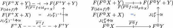
 , we define
  as the unique homomorphism from
  , we define
  as the greatest homomorphism from
In the rest of this section, we check under which conditions \(\overline{F^{+}}\) and \(\overline{F^{{\oplus }}}\) are functors and form liftings of \(F^{+}\) and \(F^{{\oplus }}\). Functoriality of \(\overline{F^{+}}\) holds if and only if for each  and
and  , \(F^{+}g\odot F^{+}f\) is the unique homomorphism from \(\overline{F}(\mathrm {id}+g)\odot \overline{F}(\mathrm {id}+f)\odot J(\iota ^F_X)^{-1}\) to \(J(\iota ^F_W)^{-1}\). Similarly, functoriality of \(\overline{F^{{\oplus }}}\) holds if and only if \(F^{{\oplus }}g\odot F^{{\oplus }}f\) is the greatest homomorphism from \(\overline{F}(\mathrm {id}+g)\odot \overline{F}(\mathrm {id}+f)\odot J\zeta ^F_X\) to \(J\zeta ^F_W\).
The former always holds by the finality. In contrast, the latter doesn’t necessarily hold: a counterexample is \(T=\mathcal {D}\) and \(F=\{o\}\times (\underline{~}\,)^2\) (see Example C.1 for details). Hence we need an extra assumption to make \(\overline{F^{{\oplus }}}\) a functor. We hereby assume a stronger condition than is needed for the sake of discussions in Sect. 4.
Definition 3.11
(\(\varPhi _{c,\sigma }\)). Let  and
and  . We define a function
  by \(\varPhi _{c,\sigma }(f):=\sigma \odot \overline{F}f\odot c\).

Definition 3.12
Assume that T and F constitute an infinitary trace situation. Let \(\zeta ^F:Z\rightarrow FZ\) be a final F-coalgebra. We say that T and F satisfy the gfp-preserving condition with respect to an \(\overline{F}\)-algebra  if for each \(X\in \mathbb {C}\) and
  , if
, if  is the greatest homomorphism from c to \(J\zeta ^F\) and the function \(\varPhi _{J\zeta ^F,\sigma }\) has the greatest fixed point
  , then
  is the greatest fixed point of \(\varPhi _{c,\sigma }\).
We next check if \(\overline{F^{+}}\) and \(\overline{F^{{\oplus }}}\) are liftings of \(F^{+}\) and \(F^{{\oplus }}\). By definition, we have \(\overline{F^{+}}JX=JF^{+}X\) and \(\overline{F^{{\oplus }}}JX=JF^{{\oplus }}X\) for each \(X\in \mathbb {C}\). Let \(f:X\rightarrow Y\). By definition, \(\overline{F^{+}}Jf=JF^{+}f\) holds if and only if \(JF^{+}f\) is a unique homomorphism from \(\overline{F}(\mathrm {id}+Jf)\odot J(\iota ^F_X)^{-1}\) to \(J(\zeta ^F_Y)^{-1}\). Similarly, \(\overline{F^{+}}Jf=JF^{+}f\) holds if and only if \(JF^{+}f\) is the greatest homomorphism from \(\overline{F}(\mathrm {id}+Jf)\odot J\zeta ^F_X\) to \(J\zeta ^F_Y\).
The former is easily proved by the finality of \(J(\iota ^F_Y)^{-1}\), while the latter requires an assumption again.
Definition 3.13
Assume T and F constitute an infinitary trace situation. Let \(\zeta ^F:Z\rightarrow FZ\) be a final F-coalgebra. We say that T and F satisfy the deterministic-greatest condition if for \(c:X\rightarrow FX\) in \(\mathbb {C}\), if \(u:X\rightarrow Z\) is the unique homomorphism from c to \(\zeta ^F\) then Ju is the greatest homomorphism from Jc to \(J\zeta ^F\).
Concluding the discussions so far, we obtain the following proposition.
Proposition 3.14
-
1.
If T and \(F(\underline{~}\,+A)\) constitute a finite trace situation for each \(A\in \mathbb {C}\), the operation \(\overline{F^{+}}\) is a functor and is a lifting of \(F^{+}\).
-
2.
If T and \(F(\underline{~}\,+A)\) constitute an infinitary trace situation and satisfy the gfp-preserving condition with respect to an arbitrary algebra and the deterministic-greatest condition for each \(A\in \mathbb {C}\), \(\overline{F^{{\oplus }}}\) is a functor and is a lifting of \(F^{{\oplus }}\).
\(\square \)
Hence under appropriate conditions, a lifting  of F gives rise to liftings of \(F^{+}\) and \(F^{{\oplus }}\). By repeating this, we can define \(\overline{F^{(i)}_{j}}\) for each i and j.
See Sect. D of the extended version [20] for the distributive laws corresponding to the liftings defined above.
Example 3.15
Let \(F=\mathsf {A}\times (\underline{~}\,)\) and \(T=\mathcal {P}\). As we have seen in Example 3.3, \(F^{+{\oplus }}X\cong (\mathsf {A}^+)^+ X+(\mathsf {A}^+)^\omega \). Let \(\overline{F}\) be a lifting that is given as in Example 2.7. We can construct a lifting \(\overline{F^{+{\oplus }}}\) using Proposition 3.14, and for  in
in  ,
,  is given by \(\overline{F^{+{\oplus }}}f(w)=\{w'y\mid y\in f(x)\}\) if \(w=w'x\) where \(w'\in (\mathsf {A}^+)^+\) and \(x\in X\), and \(\{w\}\) if \(w\in (\mathsf {A}^+)^\omega \).
4 Decorated Trace Semantics of Büchi (T, F)-systems
4.1 Definition
Assumption 4.1
Throughout this section, let T be a monad and F be an endofunctor on \(\mathbb {C}\), and assume that each homset of  carries a partial order \(\sqsubseteq \). We further assume the following conditions for each \(A\in \mathbb {C}\).
-
1.
\(F^{+},F^{+{\oplus }}:\mathbb {C}\rightarrow \mathbb {C}\) are well-defined and liftings
 are given.
 -
2.
T and \(F(\underline{~}\,+A)\) satisfy the conditions in Theorem 2.9 with respect to \(\overline{F}(\underline{~}\,+A)\) and \(\sqsubseteq \), and hence constitute a finite trace situation.
-
3.
T and \(F^{+}(\underline{~}\,+A)\) constitute an infinitary trace situation with respect to \(\overline{F^{+}}(\underline{~}\,+A)\) and \(\sqsubseteq \).
-
4.
T and \(F^{+}(\underline{~}\,+A)\) satisfy the gfp-preserving condition wrt. an arbitrary \(\sigma \).
-
5.
T and \(F^{+}(\underline{~}\,+A)\) satisfy the deterministic-greatest condition.
-
6.
The liftings \(\overline{F^{+}}\) and \(\overline{F^{+{\oplus }}}\) are obtained from \(\overline{F}\) and \(\overline{F^{+}}\) using the procedure in Definition 3.10 respectively.
-
7.
\(\overline{F^{+}}(\underline{~}\,+A)\) and \(\overline{F^{+{\oplus }}}(\underline{~}\,+A)\) are locally monotone.
-
8.
T and F constitute a Büchi trace situation with respect to \(\sqsubseteq \) and \(\overline{F}\).
 are given.
Using the categorical data type defined in Sect. 3, we now introduce a decorated Büchi trace semantics  and
and  .
.
Definition 4.2
(\(\mathsf{dtr}_i(c)\)). For a Büchi (T, F)-system \((c,(X_1,X_{2}))\), the decorated Büchi trace semantics is a solution  of the following HES (see also Eq. (2)).

Existence of a solution will be proved in the next section.
4.2 Trace Semantics vs. Decorated Trace Semantics
This section is devoted to sketching the proof of the following theorem, which relates decorated trace semantics \(\mathsf{dtr}_i(c)\) and Büchi trace semantics \(\mathsf{tr}^{\mathsf {B}}_i(c)\) in [21] via the natural transformation in Definition 3.8.
Theorem 4.3
For each \(i\in \{1,2\}\), \(\mathsf{tr}^{\mathsf {B}}_i(c)={p^{(2)}_{i\,0}}\circ \mathsf{dtr}_i(c)\). \(\square \)
To prove this, we introduce Kleisli arrows \(c_2^\ddagger \), \(\tilde{\ell }^{(1)}_1\), \(\tilde{\ell }^{(2)}_1\) and \(\tilde{\ell }^{(2)}_2\). They are categorical counterparts to \(f_2^\ddagger \), \(l^{(1)}_{1}\), \(l^{(2)}_{1}\) and \(l^{(2)}_{2}\) (see Definition 2.2) for the HES defining \(\mathsf{tr}^{\mathsf {B}}_i(c)\) (see Definition 2.13), and bridge the gap between \(\mathsf{dtr}_i(c)\) and \(\mathsf{tr}^{\mathsf {B}}_i(c)\).
Definition 4.4
(\(c_2^\ddagger \), \(\tilde{\ell }^{(1)}_1\), \(\tilde{\ell }^{(2)}_1\), \(\tilde{\ell }^{(2)}_2\)). We define Kleisli arrows  ,
,  ,
,  and
and  as follows:
-
We define
 as the unique homomorphism from an \(F(\underline{~}\,+X_2)\)-coalgebra \(c_1\) to \(J(\iota ^{F}_{X_2})^{-1}\) (see the left diagram in Eq. (4) below).
 -
We define
 by:
by: 
-
We define
 as the greatest homomorphism from \(c_2^\ddagger \) to \(J\zeta ^{F^{+}}_{0}\) (see the right diagram below).
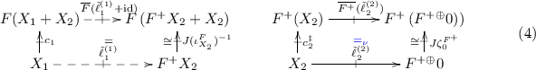
-
We define
 as follows:
 as the unique homomorphism from an
  by:
by: 
 as the greatest homomorphism from
 as follows:
We explain an intuition why Kleisli arrows defined above bridge the gap between \(\mathsf{tr}^{\mathsf {B}}_i(c)\) and \(\mathsf{dtr}_i(c)\). One of the main differences between them is that \(\mathsf{tr}^{\mathsf {B}}_1(c)\) is calculated from \(l^{(1)}_{1}(u_{2})\) which is the least fixed point of a certain function, while \(\mathsf{dtr}_1(c)\) is defined as the greatest homomorphism. The arrow \(\tilde{\ell }^{(1)}_{1}\) fills the gap because it is defined as the unique fixed point, which is obviously both the least and the greatest fixed point.
We shall prove Theorem 4.3 following the intuition above. The lemma below, which is easily proved by the finality of a, shows that not only \(\tilde{\ell }^{(1)}_{1}\) but also \(\tilde{\ell }^{(2)}_{1}\) is characterized as the unique homomorphism.
Lemma 4.5
The Kleisli arrow  is the unique homomorphism from \(\overline{F}(\mathrm {id}+\tilde{\ell }^{(2)}_{2})\odot c_1\) to \(J(\iota ^{F}_{F^{+{\oplus }}0})^{-1}\). \(\square \)

Together with the definition of \(\tilde{\ell }^{(2)}_{2}\), we have the following proposition.
Proposition 4.6
For each \(i\in \{1,2\}\), \(\tilde{\ell }^{(2)}_{i}=\mathsf{dtr}_i(c)\). \(\square \)
This proposition implies the existence of a solution of the HES in Definition 4.2.
It remains to show the relationship between the \(\tilde{\ell }^{(i)}_{j}\) and \(\mathsf{tr}^{\mathsf {p}}_i(c)\). By using that \(\tilde{\ell }^{(1)}_{1}\) is the unique fixed point (and hence the least fixed point), we can prove the following equality for an arbitrary  .
.

The following equalities are similarly proved using the equality above.

By the definition of \(\mathsf{tr}^{\mathsf {B}}_i(c)\), these equalities imply the following proposition.
Proposition 4.7
For each \(i\in \{1,2\}\), \(\mathsf{tr}^{\mathsf {B}}_i(c)={p^{(2)}_{i\,0}}\circ \tilde{\ell }^{(2)}_{i}\). \(\square \)
5 Decorated Trace Semantics for Nondeterministic Büchi Tree Automata
We apply the framework developed in Sects. 3 and 4 to nondeterministic Büchi tree automata (NBTA), systems that nondeterministically accept trees with respect to the Büchi condition (see e.g. [17]). We show what datatypes \(F^{+}(F^{+{\oplus }}0)\) and \(F^{+{\oplus }}0\), and \(\mathsf{dtr}_i(c)\) characterize for an NBTA. We first review some basic notions.
5.1 Preliminaries on Büchi Tree Automaton
Definition 5.1
(Ranked Alphabet). A ranked alphabet is a set \(\varSigma \) equipped with an arity function \(|\underline{~}\,|:\varSigma \rightarrow \mathbb {N}\). We write \(\varSigma _n\) for \(\{a\in \varSigma \mid |a|=n\}\). For a set X, we regard \(\varSigma +X\) as a ranked alphabet by letting \(|x|=0\). We also regard \(\varSigma \times X\) as a ranked alphabet by letting \(|(a,x)|=|a|\).
Definition 5.2
(\(\varSigma \)-labeled Tree, [7]). A tree domain is a set \(D\subseteq \mathbb {N}^*\) s.t.: i) \(\langle \rangle \in D\), ii) for \(w,w'\in \mathbb {N}^*\), \(ww'\in D\) implies \(w\in D\) (i.e. it is prefix-closed), and iii) for \(w\in D\) and \(i,j\in \mathbb {N}\), \(wi\in D\) and \(j\le i\) imply \(wj\in D\) (i.e. it is downward-closed). A \(\varSigma \)-labeled (infinitary) tree is a pair \(t=(D,l)\) of a tree domain D and a labeling function \(l:D\rightarrow \bigcup _{n\in \mathbb {N}}\varSigma _n\) s.t. for \(w\in D\), \(|l(w)|=n\) implies \(\{i\in \mathbb {N}\mid wi\in D\}=[0,n-1]\). A \(\varSigma \)-labeled tree \(t=(D,l)\) is finite if D is a finite set. We write \(\mathsf {Tree}_{\infty }(\varSigma )\) (resp. \(\mathsf {Tree}_{\mathsf {fin}}(\varSigma )\)) for the set of \(\varSigma \)-labeled infinitary (resp. finite) trees. For \(w\in D\), the w-th subtree \(t_w\) of t is defined by \(t_w=(D_w,l_w)\) where \(D_w:=\{w'\in \mathbb {N}^*\mid ww'\in D\}\) and \(l_w(w'):=l(ww')\). A branch of t is a possibly infinite sequence \(i_1i_2\ldots \in \mathbb {N}^\infty \) s.t. \(i_1i_2\ldots i_k\in D\) for each \(k\in \mathbb {N}\), and if it is a finite sequence \(i_1i_2\ldots i_k\) then \(|l(i_0i_1\ldots i_k)|=0\). We sometimes identify a branch \(i_0i_1\dots \in \mathbb {N}^\infty \) with a sequence \(l(\langle \rangle )l(i_1)l(i_1i_2)\dots \in \varSigma ^\infty \).
Remark 5.3
For the sake of notational simplicity, we identify a \(\varSigma \)-labeled tree with a \(\varSigma \)-term in a natural manner. For example, a \(\{a,b\}\)-term (a, (b, b)) denotes an \(\{a,b\}\)-labeled finite tree \(t=(\{\langle \rangle ,0,1\},[\langle \rangle \mapsto a,0\mapsto b,1\mapsto b])\). Moreover, for \(\{a,b,c\}\)-labeled trees \(t_0=(D_0,l_0)\) and \(t_1=(D_1,l_1)\), we write \((c,t_0,t_1)\) for a tree \(t=(\{\langle \rangle \cup \{0w\mid w\in D_0\}\cup \{1w\mid w\in D_1\}, [\langle \rangle \mapsto c, 0w\mapsto l_0(w), 1w\mapsto l_1(w)])\).
Definition 5.4
(NBTA). A nondeterministic Büchi tree automaton (NBTA) is a tuple \(\mathcal {A}=(X,\varSigma ,\delta ,\mathsf {Acc})\) of a state space X, a ranked alphabet \(\varSigma \), a transition function \(\delta :X\rightarrow \mathcal {P}(\coprod _{n\in \mathbb {N}}\varSigma _n\times X^{n})\) and a set \(\mathsf {Acc}\subseteq X\) of accepting states.
Definition 5.5
. Let \(\mathcal {A}=(X,\varSigma ,\delta ,\mathsf {Acc})\) be an NBTA. A run tree over \(\mathcal {A}\) is a \((\varSigma \times X)\)-labeled tree \(\rho \) such that for each subtree \(((a,x),((a_0,x_0),t_{00},\ldots ,t_{0n_0}),\ldots ,((a_n,x_n),t_{n0},\ldots ,t_{nn_n}))\), \((a,x_0,\ldots ,x_n)\in \delta (x)\) holds. A run tree is accepting if for each branch \((a_0,x_0)(a_1,x_1)\ldots \in (\varSigma \times X)^\omega \), \(x_i\in \mathsf {Acc}\) for infinitely many i. We write \(\mathrm {Run}_{\mathcal {A}}(x)\) (resp. \(\mathrm {AccRun}_{\mathcal {A}}(x)\)) for the set of run trees (resp. accepting run trees) whose root node is labeled by \(x\in X\). For \(A\subseteq X\), \(\mathrm {Run}_{\mathcal {A}}(A)\) denotes \(\cup _{x\in A}\mathrm {Run}(x)\). We define \(\mathrm {AccRun}_{\mathcal {A}}(A)\) similarly. If no confusion is likely, we omit the subscript \(\mathcal {A}\). We define \(\mathrm {DelSt}:\mathrm {Run}(X)\rightarrow \mathsf {Tree}_{\infty }(\varSigma )\) by \(\mathrm {DelSt}(D,l):=(D,l')\) where \(l'(w):=\pi _1(l(w))\). The language \(L^{\mathrm {B}}_{\mathcal {A}}:X\rightarrow \mathcal {P}\mathsf {Tree}_{\infty }(\varSigma )\) of \(\mathcal {A}\) is defined by \(L^{\mathrm {B}}_{\mathcal {A}}(x)=\mathrm {DelSt}(\mathrm {AccRun}_{\mathcal {A}}(x))\).
5.2 Decorated Trace Semantics of NPTA
A ranked alphabet \(\varSigma \) induces a functor \(F_{\varSigma }=\coprod _{n\in \mathbb {N}}\varSigma _n\times (\underline{~}\,)^n:\mathbf {Sets}\rightarrow \mathbf {Sets}\). In [21], an NBTA \(\mathcal {A}\) was modeled as a Büchi \((\mathcal {P},F_{\varSigma })\)-system, and it was shown that \(L^{\mathrm {B}}_{\mathcal {A}}\) is characterized by a coalgebraic Büchi trace semantics \(\mathsf{tr}^{\mathsf {B}}_i(c)\).
Proposition 5.6
([21]). For \(X,Y\in \mathbf {Sets}\), we define an order \(\sqsubseteq \) on  by \(f\sqsubseteq g{\mathop {\Leftrightarrow }\limits ^{\text {def.}}}\forall x\in X.\, f(x)\subseteq g(x)\). We define
  by \(\overline{F_{\varSigma }}X:=X\) for
  and \(\overline{F_{\varSigma }} f(a,x_1,\ldots ,x_n):=\{(a,y_1,\ldots ,y_n)\mid y_i\in f(x_i)\}\) for
  . It is easy to see that \(\overline{F_{\varSigma }}\) is a lifting of \(F_{\varSigma }\). Then we have:
-
1.
\(\mathcal {P}\) and \(F_{\varSigma }\) constitute a Büchi trace situation (Definition 2.13) with respect to \(\sqsubseteq \) and \(\overline{F_{\varSigma }}\).
-
2.
The carrier set of the final \(F_{\varSigma }\)-coalgebra is isomorphic to \(\mathsf {Tree}_{\infty }(\varSigma )\).
-
3.
For an NBTA \(\mathcal {A}=(X,\varSigma ,\delta ,\mathsf {Acc})\), we define a Büchi \((\mathcal {P},F_{\varSigma })\)-system
 by \(c:=\delta \), \(X_1:=X\setminus \mathsf {Acc}\) and \(X_2:=\mathsf {Acc}\). Then we have: \([\mathsf{tr}^{\mathsf {B}}_1(c),\mathsf{tr}^{\mathsf {B}}_2(c)]=L^{\mathrm {B}}_{\mathcal {A}}:X\rightarrow \mathcal {P}\mathsf {Tree}_{\infty }(\varSigma )\). \(\square \)
 by
by In the rest of this section, for an NBTA \(\mathcal {A}=(X,\varSigma ,\delta ,\mathsf {Acc})\) modeled as a \((\mathcal {P},F_{\varSigma })\)-system \((c:X\rightarrow \mathcal {P}F_{\varSigma }X,(X_1,X_2))\), we describe \(\mathsf{dtr}_i(c)\) and show the relationship with \(\mathsf{tr}^{\mathsf {B}}_i(c)\) using Theorem 4.3.
We first describe datatypes \(F_{\varSigma }^+(F_{\varSigma }^{+{\oplus }}0)\) and \(F_{\varSigma }^{+{\oplus }}0\) referring to the construction of a final coalgebra in Theorem 2.5. We can easily see that \(F_{\varSigma }^+A\cong \mathsf {Tree}_{\mathsf {fin}}^+(\varSigma ,A) :=\mathsf {Tree}_{\mathsf {fin}}(\varSigma +A)\setminus \{(x)\mid x\in A\}\). Hence for each \(i\in \omega \), by a similar characterization to Example 3.3, we have:

Therefore \(F_{\varSigma }^{+{\oplus }}0\), a limit of the above sequence by Theorem 2.5, and \(F_{\varSigma }^+(F_{\varSigma }^{+{\oplus }}0)\) are characterized as follows:
Proposition 5.7
We define  by:
by:

where \(i\in \{1,2\}\) and \(\bullet \) is  if \(i=1\) and
  if \(i=2\). Then \(\mathrm {AccTree}_{1}(\varSigma )\cong F_{\varSigma }^+(F_{\varSigma }^{+{\oplus }}0)\) and \(\mathrm {AccTree}_{2}(\varSigma ,A)\cong F_{\varSigma }^{+{\oplus }}0\). \(\square \)
We now show what \(\mathsf{dtr}_i(c)\) characterizes for an NBTA with respect to the characterization in Proposition 5.7. Firstly, Assumption 4.1 in the previous section is satisfied.
Proposition 5.8
Assumption 4.1 is satisfied by \((T,F)=(\mathcal {P},F_{\varSigma })\). \(\square \)
By Proposition 5.7, for \(i\in \{1,2\}\), \(\beta _{i\,0}\) (see Definition 3.4) has a type
and is given by \(\beta _{i\,A}(\xi )=(a,\xi _0,\ldots ,\xi _{n-1})\) if the root of \(\xi \) is labeled by  . Using this, we can show the following characterization of \(\mathsf{dtr}_i(c)\).
Proposition 5.9
Let \(\mathcal {A}=(X,\varSigma ,\delta ,\mathsf {Acc})\) be an NBTA. We define  by \(\varOmega (D,l):=(D,l')\) where for \(w\in D\) s.t. \(l(w)=(a,x)\),
  if \(x\notin Acc\) and
  if \(x\in Acc\). We define a Büchi \((\mathcal {P},F_{\varSigma })\)-system
  as in Proposition 5.6.3. Then for \(i\in [1,2n]\) and \(x\in X_i\),
\(\square \)
We conclude this section by instantiating \({p^{(2)}_{i\,A}}\) (Definition 3.8) for NBTAs.
Proposition 5.10
We overload \(\mathrm {DelSt}\) and define \(\mathrm {DelSt}:\mathrm {AccTree}_{1}(\varSigma )+\mathrm {AccTree}_{2}(\varSigma )\rightarrow \mathsf {Tree}_{\infty }(\varSigma )\) by \(\mathrm {DelSt}(D,l):=(D,l')\) where \(l'(w):=\pi _1(l(w))\). Then with respect to the isomorphism in Proposition 5.7, \(\mathrm {DelSt}(\xi )={p^{(2)}_{i\,A}}(\xi )\) for each \(i\in \{1,2\}\) and \(\xi \in \mathrm {AccTree}_{i}(\varSigma )\). \(\square \)
Hence Theorem 4.3 results in the following (obvious) equation for NBTAs:
6 Systems with Other Branching Types
In this section we briefly discuss other monads than \(T=\mathcal {P}\). As we have discussed in Sect. 3.3, the framework does not apply to \(T=\mathcal {D}\).
Let \(T\,{=}\,\mathcal {L}\) and \(F\,{=}\,F_{\varSigma }\). A Büchi \((\mathcal {L},F_{\varSigma })\)-system  is understood as a \(\varSigma \)-labeled deterministic Büchi tree automaton with an exception. In a similar manner to \(T=\mathcal {P}\) we can prove that they satisfy Assumption 4.1. The resulting decorated trace semantics has a type \(\mathsf{dtr}_i(c):X_i\rightarrow \{\bot \}+\mathrm {AccTree}_{i}(\varSigma )\). Note that once \(x\in X\) is fixed, either of the following occurs: a decorated tree is determined according to c; or \(\bot \) is reached at some point. The function \(\mathsf{dtr}_i(c)\) assigns \(\bot \) to \(x\in X_i\) if and only if \(\bot \) is encountered from x or the resulting decorated tree does not satisfy the Büchi condition: otherwise, the generated tree is assigned to x. See Sect. E.1 of the extended version [20] for detailed discussions, which includes the case of parity automata.
We next let \(T=\mathcal {G}\). A Büchi \((\mathcal {G},F_{\varSigma })\)-system is understood as a probabilistic Büchi tree automaton. In fact, it is open if \(T=\mathcal {G}\) and \(F=F_{\varSigma }\) satisfy Assumption 4.1. The challenging part is the gfp-preserving condition (Assumption 4.1.4). However, by carefully checking the proofs of the lemmas and the propositions where the gfp-preserving condition is used (i.e. Proposition 3.14, Lemma 4.5 and Proposition 4.7), we can show that Assumption 4.1.4 can be relaxed to the following weaker but more complicated conditions:
-
4’-1.
T and \(F^{+}(\underline{~}\,+A)\) satisfy the gfp-preserving condition with respect to
 for each
  ;
; -
4’-2.
T and
 satisfy the gfp-preserving condition with respect to an algebra
  where \(\tau \) is the unique homomorphism from
 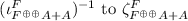 ; and
; and -
4’-3.
T and \(F(\underline{~}\,+A)\) satisfy the gfp-preserving condition with respect to an algebra
 .
.
 for each
  ;
; satisfy the gfp-preserving condition with respect to an algebra
  where
where  ; and
; and .
.In fact, only the first condition is sufficient to prove Proposition 3.14 and Lemma 4.5.
We can show that \(T=\mathcal {G}\) and \(F=F_{\varSigma }\) on \(\mathbf {Meas}\) satisfy the above weakened gfp-preserving condition, and hence we can consider a decorated trace semantics \(\mathsf{dtr}_i(c)\) for a Büchi \((\mathcal {G},F_{\varSigma })\)-system  and use Theorem 4.3.
Assume X is a countable set equipped with a discrete \(\sigma \)-algebra for simplicity. Then the resulting decorated trace semantics \(\mathsf{dtr}_i(c)\) has a type \(X_i\rightarrow \mathcal {G}(\mathrm {AccTree}_{i}(\varSigma ),\mathfrak {F}_{\mathrm {AccTree}_{i}(\varSigma )})\) where \(\mathfrak {F}_{\mathrm {AccTree}_{i}(\varSigma )}\) is the standard \(\sigma \)-algebra generated by cylinders. The probability measure assigned to \(x\in X_i\) by \(\mathsf{dtr}_i(c)\) is defined in a similar manner to the probability measure over the set of run trees generated by a probabilistic Büchi tree automaton (see e.g. [18]).
The situation is similar for parity \((\mathcal {G},F_{\varSigma })\)-systems. See [20, Sect. E.2] for details.
7 Conclusions and Future Work
We have introduced a categorical data type for capturing behavior of systems with Büchi acceptance conditions. The data type was defined as an alternating fixed point of a functor, which is understood as the set of traces decorated with priorities. We then defined a notion of coalgebraic decorated trace semantics, and compared it with the coalgebraic trace semantics in [21]. We have applied our framework for nondeterministic Büchi tree automata, and showed that decorated trace semantics is concretized to a function that assigns a set of trees decorated with priorities so that the Büchi condition is satisfied in every branch. We have focused on the Büchi acceptance condition for simplicity, but all the results can be extended to the parity acceptance condition (see Sect. A of [20] for the details).
Future Work. There are some directions for future work. In this paper we focused on systems with a simple branching type like nondeterministic or probabilistic. Extending this so that we can deal with systems with more complicated branching type like two-player games (systems with two kinds of nondeterministic branching) or Markov decision processes (systems with both nondeterministic and probabilistic branching) is a possible direction of future work.
Another direction would be to use the framework developed here to categorically generalize a verification method. For example, using the framework of coalgebraic trace semantics in [21], a simulation notion for Büchi automata is generalized in [19]. Searching for an existing verification method that we can successfully generalize in our framework would be interesting.
Finally, it was left open in Sect. 6 if Assumption 4.1.4 is satisfied by \(T=\mathcal {G}\) and \(F=F_{\varSigma }\). Investigating this is clearly a future work.
Notes
- 1.
We write
 for a Kleisli arrow
  and
and  for a lifting of the functor F over
  , for distinction.
 for a Kleisli arrow
  and
and  for a lifting of the functor F over
  , for distinction.
References
Adámek, J., Koubek, V.: Least fixed point of a functor. J. Comput. Syst. Sci. 19(2), 163–178 (1979). https://doi.org/10.1016/0022-0000(79)90026-6
Adámek, J., Milius, S., Moss, L.S.: Fixed points of functors. J. Log. Algebraic Methods Program. 95, 41–81 (2018)
Arnold, A., Niwiński, D.: Rudiments of \(\mu \)-Calculus. Studies in Logic and the Foundations of Mathematics. Elsevier, Amsterdam (2001)
Borceux, F.: Handbook of Categorical Algebra, Encyclopedia of Mathematics and its Applications, vol. 1. Cambridge University Press, Cambridge (1994)
Ciancia, V., Venema, Y.: Stream automata are coalgebras. In: Pattinson, D., Schröder, L. (eds.) CMCS 2012. LNCS, vol. 7399, pp. 90–108. Springer, Heidelberg (2012). https://doi.org/10.1007/978-3-642-32784-1_6
Cleaveland, R., Klein, M., Steffen, B.: Faster model checking for the modal mu-calculus. In: von Bochmann, G., Probst, D.K. (eds.) CAV 1992. LNCS, vol. 663, pp. 410–422. Springer, Heidelberg (1993). https://doi.org/10.1007/3-540-56496-9_32
Courcelle, B.: Fundamental properties of infinite trees. Theor. Comput. Sci. 25, 95–169 (1983). https://doi.org/10.1016/0304-3975(83)90059-2
Etessami, K., Wilke, T., Schuller, R.A.: Fair simulation relations, parity games, and state space reduction for Büchi automata. SICOMP 34(5), 1159–1175 (2005)
Ghani, N., Hancock, P., Pattinson, D.: Representations of stream processors using nested fixed points. Log. Methods Comput. Sci. 5(3) (2009)
Hasuo, I., Jacobs, B.: Context-free languages via coalgebraic trace semantics. In: Fiadeiro, J.L., Harman, N., Roggenbach, M., Rutten, J. (eds.) CALCO 2005. LNCS, vol. 3629, pp. 213–231. Springer, Heidelberg (2005). https://doi.org/10.1007/11548133_14
Hasuo, I., Jacobs, B., Sokolova, A.: Generic trace semantics via coinduction. Log. Methods Comput. Sci. 3(4) (2007)
Jacobs, B.: Trace semantics for coalgebras. Electr. Notes Theor. Comput. Sci. 106, 167–184 (2004). https://doi.org/10.1016/j.entcs.2004.02.031
Jacobs, B.: Introduction to Coalgebra: Towards Mathematics of States and Observation. Cambridge Tracts in Theoretical Computer Science. Cambridge University Press, New York (2016)
Milius, S.: Completely iterative algebras and completely iterative monads. Inf. Comput. 196(1), 1–41 (2005)
Mulry, P.S.: Lifting theorems for Kleisli categories. In: Brookes, S., Main, M., Melton, A., Mislove, M., Schmidt, D. (eds.) MFPS 1993. LNCS, vol. 802, pp. 304–319. Springer, Heidelberg (1994). https://doi.org/10.1007/3-540-58027-1_15
Power, J., Turi, D.: A coalgebraic foundation for linear time semantics. Electr. Notes Theor. Comput. Sci. 29, 259–274 (1999)
Thomas, W.: Languages, automata, and logic. In: Rozenberg, G., Salomaa, A. (eds.) Handbook of Formal Languages, pp. 389–455. Springer, Heidelberg (1997). https://doi.org/10.1007/978-3-642-59126-6_7
Urabe, N., Hasuo, I.: Coalgebraic infinite traces and Kleisli simulations. CoRR abs/1505.06819 (2015). http://arxiv.org/abs/1505.06819
Urabe, N., Hasuo, I.: Fair simulation for nondeterministic and probabilistic Buechi automata: a coalgebraic perspective. LMCS 13(3) (2017)
Urabe, N., Hasuo, I.: Categorical Büchi and parity conditions via alternating fixed points of functors. arXiv preprint (2018)
Urabe, N., Shimizu, S., Hasuo, I.: Coalgebraic trace semantics for Büchi and parity automata. In: Proceedings of the CONCUR 2016. LIPIcs, vol. 59, pp. 24:1–24:15. Schloss Dagstuhl - Leibniz-Zentrum fuer Informatik (2016)
Acknowledgments
We thank Kenta Cho, Shin’ya Katsumata and the anonymous referees for useful comments. The authors are supported by JST ERATO HASUO Metamathematics for Systems Design Project (No. JPMJER1603), and JSPS KAKENHI Grant Numbers 15KT0012 & 15K11984. Natsuki Urabe is supported by JSPS KAKENHI Grant Number 16J08157.
Author information
Authors and Affiliations
Corresponding author
Editor information
Editors and Affiliations
Rights and permissions
Copyright information
© 2018 IFIP International Federation for Information Processing
About this paper

Cite this paper
Urabe, N., Hasuo, I. (2018). Categorical Büchi and Parity Conditions via Alternating Fixed Points of Functors. In: Cîrstea, C. (eds) Coalgebraic Methods in Computer Science. CMCS 2018. Lecture Notes in Computer Science(), vol 11202. Springer, Cham. https://doi.org/10.1007/978-3-030-00389-0_12
Download citation
DOI: https://doi.org/10.1007/978-3-030-00389-0_12
Published:
Publisher Name: Springer, Cham
Print ISBN: 978-3-030-00388-3
Online ISBN: 978-3-030-00389-0
eBook Packages: Computer ScienceComputer Science (R0)