Wave Theory of Image Formation in a Microscope: Basic Theory and Experiments

Abstract

Biology is intimately linked with microscopy. The cell theory that underpins all of biology traces its roots back to Leeuwenhoek’s development of the first practical microscope. Many of us use the terms “numerical aperture” and “working distance” in the lab and know, as a rule of thumb, to use short wavelengths for illumination to maximize resolution. But when pressed we must confess a poor understanding of these terms and the physical basis for the rule of thumb. This chapter combines theory and simple experiments to provide a basic understanding of how images are formed and how resolution, numerical aperture, working distance, and wavelength are interrelated.

Appendices

Problems

• 1.1. Calculate the line spacing d of your diffraction grating using your measurements of X and Y _m (Table 1.2).

  Table 1.2 Differences in ${Y}_{\pm m}$ values due to misalignment of laser and object

• 1.2. Find the FT of a 2D array of sources at $x=0$ arranged in a rectangular pattern with y spacing of ℓ _y and z spacing of ℓ _z .

• 1.3a. Explain both qualitatively and quantitatively why in Fig. 1.10 the central spot, and only the central spot, is white (Fig. 1.19).

  Fig. 1.19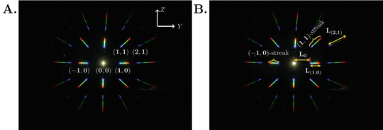

  

  Images for Problem 1.3. Diffraction pattern from rainbow glasses illuminated by a halogen lamp

• 1.3b. Explain why some of the light streaks are at an angle to the horizontal and vertical axes. Calculate what the angle of these light streaks should be and compare them to measurements taken from the figure.

• 1.3c. Calculate the approximate length of the streaks and compare them to the measurements taken from the figures.

• 1.4. Prove that ψ(N, ξ) attains its maximum when $\xi = m\lambda$.

• 1.5. Prove that the sinc function behaves as a Dirac delta function.

  The integral Si(x) (called sinint in MATLAB) is

  $$ \mathrm{S}\mathrm{i}(x)={\displaystyle {\int}_0^x}\frac{sinz}{z}\kern0.5em d z. $$

  When $x=\infty$, $\mathrm{S}\mathrm{i}\left(\infty \right)=\pi /2$ [6]. To establish the sieving property of sin(k _Y z)/z we want to show that most of the contribution to the integral

  $$ {\displaystyle {\int}_{-\infty}^{\infty }}\frac{ \sin {k}_Y z}{z} f(z)\kern0.5em d z $$

  occurs in a small region between $-\varepsilon < z<\varepsilon$ when k _Y is large enough.

  In other words, given any $\varepsilon >0$ we can choose k _Y large enough such that

  $$ {\displaystyle {\int}_{-\varepsilon}^{\varepsilon}}\frac{ \sin {k}_Y z}{z} f(z)\kern0.5em d z\sim f(0). $$

  (1.57)

Solution

• 1.1. Set up your laser and object as shown in Fig. 1.1. The number of diffraction spots you see will depend on the object. If you are using a CD you may only see the central maximum and the two secondary maxima as seen in Fig. 1.3. Measure the distance between the central and secondary maxima Y ₁ and ${Y}_{-1}$ and as many other distances as possible or convenient. If Y _m varies significantly from ${Y}_{- m}$ it probably means that the plane of the object is not perpendicular to the laser beam. Use the alignment tip to get the plane of the object perpendicular to the laser beam. For example, the following table shows our measurements before (column 2) and after (column 3) alignment. The effect of misalignment is prominent for ${Y}_{\pm 2}$. In this case we used a CD, a green laser (${\lambda}_0=532\;\mathrm{nm}$), and the distance between the CD and wall was $X=69\;\mathrm{cm}$.

  We calculate the distance between the scattering objects, d, using Eq. (1.11). Since the experiment is done in air we set the refractive index n _D to 1. λ ₀ will depend on the laser you use, typically 532 nm for green and 670 nm for red. sin θ _m is given by Eq. (1.9). For example, to find sin θ ₁, average the Y ₁ and ${Y}_{-1}$ values; in our case 25.9 cm. Thus,

  $$ \sin {\theta}_1=\frac{25.9}{\sqrt{69^2+{25.9}^2}}=0.35. $$

  d is found using Eq. (1.11),

  $$ d=\frac{m{\lambda}_0}{n_D \sin {\theta}_1}=\frac{1.532\;\mathrm{nm}}{1.0\times 0.35}=1.5\kern0.5em \upmu \mathrm{m}. $$

  This value of 1.5 μm is close to the CD track spacing of 1.6 μm measured with an electron microscope [5]. You should calculate d using the data for ${Y}_{\pm 2}$ given in the table.

• 1.2. The FT of an arbitrary object is given by Eqs. (1.47) and (1.48). We treat the 2D array of sources as Dirac delta functions so we write the field source as

  $$ \varepsilon \left( x=0, y, z\right)={\varepsilon}_0{\displaystyle \sum_{j=- N}^N{\displaystyle \sum_{k=- M}^M\delta \left( y-{y}_j\right)\delta \left( z-{z}_k\right)}}, $$

  (1.58)

  where ${y}_j= j{\ell}_y$ and ${z}_k= k{\ell}_z$ are the location of the scatterers. Because the Dirac delta functions have the sieving property, the integrals in Eq. (1.47) are easy to evaluate. The FT of $\varepsilon \left( x=0, y, z\right)$ is

  $$ \widehat{\varepsilon}\left({k}_Y,{k}_Z\right)={\varepsilon}_0{\displaystyle \sum_{j=- N}^N{\displaystyle \sum_{k=- M}^M{\mathrm{e}}^{i{ y}_j{k}_Y}{\mathrm{e}}^{i{ z}_k{k}_Z}}}. $$

  (1.59)

  Because each term in the summation depends only on y or z but not both, we can evaluate the sums separately. Let us work on the y summation; the summation on z will be exactly the same. Recall from Eq. (1.46) that

  $$ {k}_Y\equiv \frac{ k Y}{R}=\frac{2\pi Y}{\lambda R} $$

  and substituting ${y}_j= j{\ell}_y$ we see that the exponent is

  $$ i j\left({\ell}_y\frac{2\pi Y}{\lambda R}\right)\equiv i j\cdot 2\xi (Y). $$

  The reason for defining ξ(Y) as

  $$ \xi (Y)=\frac{\ell_y\pi Y}{\lambda R} $$

  is for purely esthetic reasons. The y sum becomes (where we understand that $\xi =\xi (Y)$)

  $$ {\displaystyle \sum_{j=- N}^N{\mathrm{e}}^{ij{\ell}_y{k}_Y}}={\displaystyle \sum_{j=- N}^N{\mathrm{e}}^{2 ij\xi}}=\frac{ \sin \left[\left(2 N+1\right)\xi \right]}{ \sin \left(\xi \right)}=\psi \left(\xi, 2 N+1\right). $$

  Note that we get the same ψ function as in the case of $N+1$ scatterers on a line. Had we defined $\xi =2\pi {\ell}_y Y/\left(\lambda R\right)$ the sine argument of the numerator would have been $\left( N+1/2\right)$, which is, to us, esthetically unpleasing but perfectly correct.

  Now we can write $\widehat{\varepsilon}\left({k}_Y,{k}_Z\right)$ as

  $$ \widehat{\varepsilon}\left({k}_Y,{k}_Z\right)={\varepsilon}_0\cdot \psi \left(\xi (Y),2 N+1\right)\cdot \psi \left(\xi (Z),2 M+1\right). $$

  In Problem 1.4 you showed that $\psi \left(\xi, 2 N+1\right)$ has its extrema at $\xi = n\pi$. Therefore, the diffraction spots occur when Y _n and Z _m satisfy

  $$ \frac{\ell_y\pi {Y}_n}{\lambda R}= n\pi \kern1em \mathrm{and}\kern1em \frac{\ell_z\pi {Z}_m}{\lambda R}= m\pi . $$

  In other words,

  $$ {Y}_n=\frac{ n\lambda R}{\ell_y}\kern1em \mathrm{and}\kern1em {Z}_m=\frac{ m\lambda R}{\ell_z}. $$

• 1.3a. The (n, m) indices of the diffraction spots are labeled in Fig. 1.19a. These indices correspond to Y _n and Z _m . The central maximum, (0,0), is where the light is not diffracted so light of all frequencies generated by the lamp arrive at this one spot. Therefore, this one spot is white. For any other diffraction spots, $n\ne 0$ or $m\ne 0$ in Eq. (1.49), the position of the maxima is wavelength dependent. The next problem quantifies this phenomenon.

• 1.3b. For convenience we define an (n, m)-streak as the band of light emanating from index (n, m) as shown in Fig. 1.19b. The position of the (n, m) diffraction maximum is given by Eq. (1.49), which we repeat here for convenience:

  $$ {Y}_n=\frac{ n R\lambda}{\ell_y}\kern1em \mathrm{and}\kern1em {Z}_m=\frac{ m R\lambda}{\ell_z}. $$

  Note that the position depends continuously and linearly on the wavelength λ. Therefore, if we imagine continuously changing the wavelength of light we would see the position of the maximum moving linearly. The colored banded streak reveals the wavelength-dependent maxima. The slope of the (n, m)-streak is

  $$ \frac{d{ Z}_m}{d{ Y}_n}=\frac{\frac{\partial {Z}_m}{\partial \lambda}}{\frac{\partial {Y}_n}{\partial \lambda}}=\frac{m}{n}\frac{\ell_y}{\ell_z}. $$

  From Fig. 1.9 and our earlier discussion we know that the diffraction maxima are equally spaced along Y and Z, which implies that ${\ell}_y={\ell}_z$. Therefore, the slope of the (n, m)-streak is simply m/n. The slope of the (1, 1)-streak is 1 so the angle is 45° and the slope of the (2, 1)-streak is 1/2 and the angle is ${\displaystyle { \tan}^{-1}}\left(1/2\right)=26.6{}^{\circ}$. The angles we measured from the image are 45° and 28°.

• 1.3c. The length of Y _n (λ) and Z _m (λ) (Eq. (1.49)) will depend on the range of wavelengths generated by the lamp. We see in Fig. 1.19 colors ranging from red to blue. Let us assume that maximum wavelength corresponds to red, ${\lambda}_{\max }=670\;\mathrm{nm}$ and the shortest wavelength to blue, ${\lambda}_{\min }=450\;\mathrm{nm}$. Define

  $$ \Delta {Y}_n=\frac{ n R}{\ell}\left({\lambda}_{\max }-{\lambda}_{\min}\right)\kern1em \mathrm{and}\kern1em \Delta {Z}_m=\frac{ m R}{\ell}\left({\lambda}_{\max }-{\lambda}_{\min}\right). $$

  The absolute length depends on $\rho = R/\ell$ but we do not know, X, the distance between the rainbow glasses and the camera’s sensor therefore R is unknown. Therefore, we will calculate the length of the (1, 0)-streak relative to the distance between the central maximum (0,0) and ${Y}_1\left(\lambda =450\right)$, the position of the blue tip of the (1,0)-streak.

  The length of the (1,0)-streak is

  $$ {L}_{\left(1,0\right)}=\Delta {Y}_1=\rho \Delta \lambda . $$

  The distance between the central maximum and the blue tip of the (1,0)-streak is

  $$ {L}_0={Y}_1\left(450\kern0.5em \mathrm{nm}\right)-{Y}_0=450\rho . $$

  Therefore, the length of L _(1,0) relative to L ₀ is

  $$ \frac{L_{\left(1,0\right)}}{L_0}=\frac{\left(670-450\right)\rho}{450\rho}=0.4. $$

  Hand measurement gives ${L}_{\left(1,0\right)}/{L}_0=0.45$, close to the predicted value.

  Length of the (2,1)-streak, L _(2,1) . L _(2,1) is the length of the hypothenuse of the right triangle whose base is $\Delta {Y}_2=2\rho \Delta \lambda$ and height is $\Delta {Z}_1=\rho \Delta \lambda$. Therefore,

  $$ {L}_{\left(2,1\right)}=\sqrt{\Delta {Y}_2^2+\Delta {Z}_1^2}=\sqrt{5}\rho \Delta \lambda . $$

  The length of L _(2,1) relative to L _(1,0) is $\sqrt{5}\rho \Delta \lambda /\left(\rho \Delta \lambda \right)=\sqrt{5}$.

  On our screen, L _(1,0) is 0.40 in. and the measured length of L _(2,1) is 0.89 in. The ratio is $0.89/0.40=2.21\approx \sqrt{5}=2.24$.

• 1.4. Proof.

  We will just show the maximum part. sin Nx achieves its maximum value of 1 at $x=\pi /\left(2 N\right)$. Beyond that, sin Nx is decreasing while sin x is still increasing so ψ(N, x) must decrease for $x>\pi /\left(2 N\right)$. Therefore, it suffices to consider the domain $0< x\le \pi /\left(2 N\right)$.

  Suppose there exists an $x\in \left(0,\pi /2 N\right]$ such that $\psi \left( N, x\right)\ge N$ then equivalently, $\sin N x\ge N \sin x$. We know that equality holds at $x=0$ and that for $x>0$, the slope of sin Nx, N cos Nx, is less than the slope of N sin x, N cos x. This means that for a region about $x=0$, $\sin N x\ge N \sin x$. Therefore, if there is some $0< x<\pi /2 N$ where $\sin N x> N \sin x$ then the slope of sin Nx must have started to increase, which means that there is a point where the slope of sin Nx is zero. But the slope is zero only at π/2N. Therefore, there could be no x on $\Big(0,\pi /2 N\Big]$ where $\psi \left( N, x\right)\ge N$.

• 1.5. Proof.

  Make the change of variables $w={k}_Y z$ then

  $$ {\displaystyle {\int}_{-\varepsilon}^{\varepsilon}}\frac{ \sin {k}_Y z}{z} f(z)\kern0.5em d z={\displaystyle {\int}_{-{k}_Y\varepsilon}^{k_Y\varepsilon}}\frac{ \sin w}{w} f\left(\frac{w}{k_Y}\right)\kern0.5em d w. $$

  (1.60)

  Now because $w\in \left[-{k}_Y\varepsilon, {k}_Y\varepsilon \right]$ it follows that the argument of f is within $\left[-\varepsilon, \varepsilon \right]$. Assuming f is continuous then for any $\delta >0$ we can choose $\varepsilon >0$ such that $\left| f(w)- f(0)\right|<\delta$. This means we can then replace f(w/k _Y ) by f(0)

  $$ {\displaystyle {\int}_{-{k}_Y\varepsilon}^{k_Y\varepsilon}}\frac{ \sin w}{w} f\left(\frac{w}{k_Y}\right)\kern0.5em d w\approx f(0){\displaystyle {\int}_{-{k}_Y\varepsilon}^{k_Y\varepsilon}}\frac{ \sin w}{w}\kern0.5em d w=2 f(0)\mathrm{S}\mathrm{i}\left({k}_Y\varepsilon \right). $$

  Having picked $\varepsilon >0$ we can choose k _Y large enough so that Si(k _Y ε) is as close to π/2 as we want.

  Therefore,

  $$ {\displaystyle {\int}_{-\infty}^{\infty }}\frac{ \sin {k}_Y z}{z} f(z)\kern0.5em d z\to \pi f(0)\ \mathrm{a}\mathrm{s}\ {k}_Y\to \infty . $$

  Note that by a simple change of variable, we get

  $$ {\displaystyle {\int}_{-\infty}^{\infty }}\frac{ \sin {k}_Y\left( z+ a\right)}{z+ a} f(z)\kern0.5em d z\to \pi f\left(- a\right)\ \mathrm{a}\mathrm{s}\ {k}_Y\to \infty . $$

  For whatever value of z that makes the argument in $\frac{ \sin\;{k}_Y\left(z+a\right)}{z+a}$ zero the integral will return πf(z).

Further Study

• 1. Born and Wolf’s Principles of Optics is the classic optics text and I highly recommend it to you. On first glance the mathematics might seem formidable but the clarity of the explanations of the physical principles is unsurpassed. Concepts that I struggled with from reading other texts became immediately clear after studying Born and Wolf.

• 2. Lipson et al. have nice experiments in the Appendices and the explanations in main text are clear.

• 3. There are great resources on the web. The interactive tutorials are tremendous pedagogical tools. Here are two that you should visit:

  • (a) The High Magnetic Field Laboratory at Florida State University website http://micro.magnet.fsu.edu

    Here you can check out the following (among many other interesting) links:

    • Basic concepts in optical microscopy http://olympus.magnet.fsu.edu/primer/anatomy/anatomy.html

    • Laser scanning confocal microscopy simulator http://olympus.magnet.fsu.edu/primer/java/confocalsimulator/index.html

  • (b) Nikon’s Microscopy University website http://www.microscopyu.com

    • Basic concepts and formulas in microscopy. There are a host of links and interactive tutorials on such topics as numerical aperture, resolution, coverslip correction, etc. http://www.microscopyu.com/articles/formulas/index.html

    • Confocal microscopy http://www.microscopyu.com/articles/confocal/index.html

• 4. Finally, do it yourself! The best way to learn about optics and microscopy is to play with them. Get yourself a laser pointer, do the experiments covered in this chapter, think deeply about what you see, wrestle with coming up with your own explanations, enjoy, and learn.

References

Davidson, M.W.: Molecular expressions. Optical microscopy primer. Museum of microscopy. http://micro.magnet.fsu.edu/primer/museum/leeuwenhoek.html
Born, M., Wolf, E.: Principles of Optics, 7th edn. Cambridge University Press, Cambridge (2009)
Lipson, S.G., Lipson, H., Tannhauser, D.S.: Optical Physics, 3rd edn. Cambridge University Press, Cambridge (1995)
Hecht, E.: Optics, 4th edn. Addison-Wesley, Boston (2001)
Hammouri, G., Dana, A., Sunar, B.: CDs have fingerprints too. In: Proceedings of the 11th Workshop on Cryptographic Hardware and Embedded Systems (CHES 2009), pp. 348–362 (2009).
Titchmarsh, E.C.: The Theory of Functions, 2nd edn. Oxford University Press, Oxford (1983)
Author information
Authors and Affiliations
Corresponding author
Editor information
Editors and Affiliations