Some Exact Solutions

Abstract

The Navier–Stokes equations are the most famous and perhaps the most important equations in fluid mechanics. In biofluid mechanics, these equations can be used to compute the flow of air within the airways, the flow of blood in large vessels at sufficiently high shear rates, the flow of urine from the bladder, the flow of crystalloid perfusates in in vitro experiments, and so on. Because few analytical solutions are available, one must often resort to numerical methods to solve these important equations. Nonetheless, in this chapter, we will consider five important analytical solutions to the Navier–Stokes equations.

Appendix 9: Biological Parameters

Fundamental to computations in mechanics is knowledge of geometry, material properties, and applied loads for the system of interest. Here, we list information of importance to hemodynamics and airflow mechanics.

Table A9.1 Values for blood pressure in humans in health and hypertension.

Table A9.2 Mean blood vessel characteristics (man).

Table A9.3 Hemodynamic characteristics (man).

Table A9.4 Mean airway characteristics (man).

Table A9.5 Ventilation–perfusion ratios.

Table A9.6 Density and viscosity for common fluids.

Exercises

• 9.1 Design (sketch) an experimental setup that ensures a constant steady flow within a parallel-plate device. Discuss various options with regard to how to generate the requisite constant pressure gradient.

• 9.2 The velocity profile in Eq. (9.15) represents a flow between parallel plates relative to an (o; x, y) coordinate system with the origin at the bottom plate. Show that the solution can alternatively be written as

  $$ {v}_x(y)=-\frac{1}{2\mu}\left(\frac{dp}{dx}\right)\left(\frac{h^2}{4}-{y}^2\right) $$

  if the origin of the coordinate system is at the centerline (i.e., y ∈ [−h/2, h/2]). Show, too, that regardless of the particular coordinate system used, the values of Q and τ _w are the same for this Poiseuille flow.

• 9.3 To facilitate access to the cells, some researchers use a parallel flow setup in an incubator wherein the bottom plate is stationary but the top surface of the fluid is exposed to an air/CO₂ environment (i.e., a free surface). Assuming a steady, incompressible, fully developed, 1-D flow, show that

  $$ Q=-\frac{h^3w}{3\mu}\left(\frac{dp}{dx}\right)\kern3pt \mathrm{and}\kern4pt {\tau}_w=\frac{3\mu Q}{w{h}^2}. $$

• 9.4 A constant-pressure gradient dp/dx = 0.2 kPa/m is used to drive glycerin through a parallel-plate device with gap h ~ 0.2 m. Find the maximum velocity and volumetric flow rate per unit width. Compare these values to those for water. Assume that the temperature is ~20 °C. Values for the viscosities are in Appendix 9.

• 9.5 Is the flow field in Example 9.2 irrotational?

• 9.6 Assuming a steady flow with no gravity, find the velocity in the x direction for the problem in Fig. 9.23, where U is constant and the fluid is at a constant pressure.

  

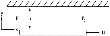
  Figure 9.23

• 9.7 Solve for the flow between parallel plates (cf. Example 9.2) with both dp/dx ≠ 0 (i.e., p ₁ > p ₂) and U ₀ ≠ 0. Calculate Q and v _x )_max, as well as σ _xy and τ _w in terms of Q.

• 9.8 For the problem in Example 9.3, show that

  $$ Q=\frac{\rho g \sin \theta {h}^3}{3\mu }. $$

  Furthermore, plot the velocity distribution v _x /v _x )_max on the abscissa versus the depth of the fluid (y/h) on the ordinate. Note that both variables are nondimensional and that they will vary from 0 to 1 regardless of the specific values in the problem. Finally, plot a normalized shear stress σ _xy /σ _xy )_max versus y/h and discuss based on the shape of the velocity distribution curve.

• 9.9 A biomedical device is thrombogenic and thus must be coated with a thin biocompatible film as in Fig. 9.24. Assume that the fluid adheres to the device (no slip) as the device is pulled through it. Assume a constant film thickness h, and that the fluid behaves as Newtonian and incompressible. By solving Navier–Stokes, show that

  

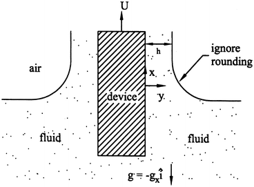
  Figure 9.24

  $$ h=\sqrt{\frac{2\mu U}{\rho {g}_x}}. $$

  Hint: Assume v _x (y = h) = 0 in addition to the free-surface boundary condition ∂v _x /∂y (y = h) = 0. What is implied by the latter condition?

• 9.10 A plate with area A and mass M is sliding down an incline covered by a fluid film of constant thickness h (Fig. 9.25). (a) Determine the velocity profile in the fluid. (b) Determine the velocity of the plate U. Hint: Assume that the pressure gradient in the x direction is zero. Draw a free-body diagram of the plate and sum the forces to find an expression for the shear stress acting on the plate in terms of M, A, and g.

  

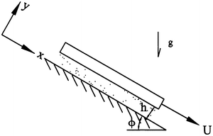
  Figure 9.25

• 9.11 A rigid membrane with negligible thickness is located between two belts and is free to move (Fig. 9.26). The top belt is moving to the right with velocity 2 U. The bottom belt is moving to the left with velocity U. The fluid in section 1 (lower-half) has viscosity μ ₁ and the fluid in section 2 (upper-half) has viscosity μ ₂, with μ ₁ = 3 μ ₂. (a) Determine the velocity field in sections 1 and 2. (b) Determine the velocity of the membrane using the given coordinate system. Hint: Draw a free-body diagram of the membrane to find the boundary condition at y = h.

  

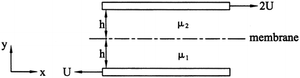
  Figure 9.26

• 9.12 A fluid film of constant thickness h is sliding down a vertical wall (Fig. 9.27). Show that the velocity field is given by

  

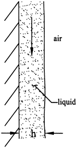
  Figure 9.27

  $$ {v}_y=\frac{\rho g{h}^2}{\mu}\left[\frac{x}{h}-\frac{1}{2}{\left(\frac{x}{h}\right)}^2\right] $$

  for x ∈ [0, h]. Hint: Assume no-slip at the wall (x = 0) and assume that the shear stress due to the airflow over the fluid is negligible (i.e., ∂v _y /∂x| _x=h  = 0). Show that the velocity field is equivalent to that obtained in Example 9.3 if θ = 90°.

• 9.13 Show that the governing differential equation [Eq. (9.39)] for a steady flow of a Newtonian fluid in a rigid circular tube can be written as

  $$ \frac{1}{\mu}\frac{dp}{dz}=\frac{d^2{v}_2}{d{r}^2}+\frac{1}{r}\frac{d{v}_z}{dr}. $$

  Consequently, the equation can be solved by assuming a solution of the form v _z ∝ r ⁿ. Show that the solution is the same as that in Eq. (9.45).

• 9.14 Ex vivo perfusion systems are becoming more common in vascular research. Assuming a fully developed laminar flow, the wall shear stress in the perfused vessel is estimated by

  $$ {\tau}_w=\frac{4\mu Q}{\pi {r}_i^3}. $$

  If r _i  ~ 2.2 mm (porcine carotid) and μ = 4 cP (Han and Ku 2001) find the value of Q necessary to produce a physiologic wall shear stress ~1.5 Pa.

• 9.15 Estimate the value of the Reynolds’ number in the vena cava in a human. For comparison, note that for the vena cava of a dog, the diameter is ~1.25 cm, the mean velocity ~33 cm/s, the wall shear rate ~211 s⁻¹, the viscosity ~3 cP, and, thus, τ _w ~0.63 Pa. What is the associated value of the skin friction coefficient c _f ?

• 9.16 Both in vivo and in vitro experiments show that the erythrocytes in blood vessels do not distribute themselves evenly across the cross section of a large blood vessel. Instead, they tend to accumulate along the centerline, thereby allowing, in a statistical sense, a thin cell-free layer to form along the wall of the vessel called the plasma layer (Fig. 9.28). Let the central core region containing cells have a viscosity μ _c and the cell-free plasma layer have a viscosity μ _p and thickness δ. In each region, assume that the flow is Newtonian. Use the Navier–Stokes equation to find (a) the velocity profile in the core region v ^c _z (r), (b) the velocity profile in the plasma layer v ^p _z (r), (c) the core volumetric flow rate Q _c , and (d) the plasma layer volumetric flow rate Q _p . Hint: Assume steady, unidirectional flow with a pressure gradient in the z direction to drive the flow. The velocity and shear stress in each region must be the same at the interface r = a – δ.

  

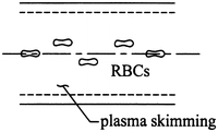
  Figure 9.28

• 9.17 For a pressure-driven axial flow between long concentric cylinders (similar to that in Fig. 9.14 but for an axial flow; see Fig. 9.29), find the expression for the velocity profile in the z direction if the inner cylinder is of radius b and outer cylinder is of radius a. This problem relates to flow in an airway or blood vessel in which a central catheter has been placed. In particular, show that (Slattery 1981)

  

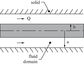
  Figure 9.29

  $$ {v}_z(r)=\frac{-{a}^2}{4\mu}\left(\frac{dp}{dz}\right)\left(1-\frac{r^2}{a^2}+\frac{1-{\beta}^2}{ \ln \left(1/\beta \right)} \ln \frac{r}{a}\right), $$

  where b = βa and β < 1. In addition, find an expression for the volumetric flow rate Q. Note that b = 0 recovers Eq. (9.45).

• 9.18 The viscosity in a concentric cylinder viscometer was shown to be calculated via

  $$ \mu =\frac{T\left({b}^2-{a}^2\right)}{4\pi \omega h{a}^2{b}^2}, $$

  where T is the applied torque, a and b are the inner and outer radii, respectively, h is the height, and ω is the angular velocity. In contrast, a so-called capillary viscometer allows one to measure viscosity according to

  $$ \mu =\frac{-\pi {a}^4}{8Q}\left(\frac{dp}{dz}\right), $$

  where dp/dz is the applied pressure gradient, a is the radius of the capillary (i.e., straight tube), and Q is the volumetric flow rate. Show that this equation is correct and state the associated restrictions that govern the experimental setup.

• 9.19 We have seen that there are many different types of viscometers, including the concentric-cylinder (Sect. 9.3) and the cone-and-plate (Sect. 7.6) devices. Explain how the results of Sect. 9.2 can be used to design a “capillary viscometer.” Also discuss why, in contrast to the cone-and-plate viscometer, the capillary viscometer would not be useful for non-Newtonian fluids.

• 9.20 Similar to the previous exercise, explain how the results of Sect. 9.1 can be used to design a parallel-plate flowmeter to measure Q.

• 9.21 Synthecon, Inc. is a company that produces rotary cell culture systems, or bioreactors. According to literature on their website, a bioreactor is any device that monitors and controls the environment of a population of cells so as to promote normal metabolic and other activities. They write further that “the fluid-filled rotating wall vessel (RWV) bioreactor is a recently developed cell culture device that is able to successfully integrate cell–cell and cell–matrix co-localization and three-dimensional interaction with excellent low-shear mass-transfer of nutrients and wastes, without sacrificing one parameter for the other. Designed by Ray Schwarz, David Wolf, and Tinh Trinh at the Johnson Manned Spaceflight Center, the RWV bioreactor consists of a cylindrical growth chamber that contains an inner co-rotating cylinder with a gas exchange membrane.” Write a three-page summary and critique of the NASA RWV bioreactor with particular emphasis on the fluid mechanics.

• 9.22 The velocity field for the NASA bioreactor (rotating cylinders) was assumed to be v = v _θ (r)ê _θ , with v _θ  = rω. This flow was shown to be “shearless” but not irrotational. How would the situation change if the angular velocity was a function of time [i.e., ω = ω(t), with both cylinders still moving together]? Why? Is it possible to construct a Womersley-type solution for an oscillating case?

• 9.23 Confirm the result in Eq. (9.84) for the error in the inferred torques based on the exact versus flat plate approximations.

• 9.24 Let b = a + h in Eq. (9.84). Show numerically how the error increases as the gap h increases. Hint: Consider different values of h as a percentage of a and plot the error versus h/a.

• 9.25 In some cases, the pressure gradient in a tube flow is computed as –∂p/∂z = Δp/L, where Δp is called the pressure drop (Δp = p _i  – p _o , where subscripts i and o denote inlet and outlet) and L is the distance between the locations at which p _i and p _o are measured. If the straight tube is angled upward at angle α, show that the results from Sect. 9.2 hold provided that the pressure gradient is taken to be (Slattery 1981, p. 73)

  $$ -\frac{\partial p}{\partial z}=\frac{p_i-{p}_o-\rho gL \sin \alpha }{L}. $$

• 9.26 A catheter is to be coated by a nonthrombogenic film. A schema of the manufacturing setup is shown in Fig. 9.30. Assume that the flow is steady, laminar, and fully developed in the section L and that the coating fluid is Newtonian. Find the volumetric flow rate Q of the fluid through this section. Assuming the coating (film) thickness δ is uniform, find an expression for δ.

  

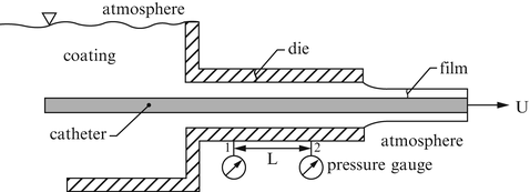
  Figure 9.30

• 9.27 In Sect. 9.4, we found the solution to the flow in an elliptical cross section by assuming a form of v _z (x, y) that satisfies the no-slip boundary condition exactly. Rederive the solution for steady, incompressible, fully developed, Newtonian flow in a rigid, straight, circular tube using this same idea. Hint: Let v _z (r) = c(x ² + y ² – a ²) = c(r ² – a ²).

• 9.28 We found that the velocity in an elliptical cross section is given by

  $$ {v}_z\left(x,y\right)=-\frac{1}{2\mu}\left(\frac{dp}{dz}\right)\frac{a^2{b}^2}{a^2+{b}^2}\left(1-\frac{x^2}{a^2}-\frac{y^2}{b^2}\right). $$

  Show that, as reported by Zamir (2000), the volumetric flow rate and wall shear stress are given by

  $$ Q=-\frac{\pi {a}^3{b}^3}{4\mu \left({a}^2+{b}^2\right)}\left(\frac{dp}{dz}\right) $$

  and

  $$ {\tau}_w=\frac{dp}{dz}\left(\frac{a^2{b}^2}{a^2+{b}^2}\right)\sqrt{\frac{x_1^2}{a^4}+\frac{y_1^2}{b^4}}, $$

  where (x ₁, y ₁), are points on the elliptical boundary.

• 9.29 The Fourier series representation for pressure in Eq. (9.97) can be written alternatively as

  $$ p(t)={p}_m+{\displaystyle \sum_{n=1}^N{C}_n\; \cos \left(\frac{2\pi nt}{T}+{\Phi}_n\right)}, $$

  where T is the period (not temperature) and Ф _n is a phase shift. Prove that this is the case, and in so doing, relate the Fourier coefficients A _n and B _n to the amplitude C _n and the phase Ф _n . See Table 9.1.

• 9.30 Plot the function

  $$ f(t)={\displaystyle \sum_{n=1}^N{C}_n\; \cos \left(\frac{2\pi nt}{T}+{\Phi}_n\right)} $$

  given

  C n	7.5803	5.4124	1.5210	0.5217	0.8311
  Ф n	−173.9200	88.9220	−21.7046	−33.5370	−126.8100

  Pick a constant value of 2π/T for a typical cardiac cycle.

• 9.31 Nagel et al. (J Clin Invest 94: 885–891, 1994) used a cone-and-plate device to subject cultured endothelial cells to various shear stresses. They showed that cultured human umbilical vein endothelial cells (HUVEC) exhibit time-dependent changes in the production of adhesion molecules for wall shear stresses τ _w from 0.25 to 4.6 Pa. They report that τ _w was given by

  $$ {\tau}_w=\frac{\mu \omega }{\alpha}\left[1-0.4743{\left(\frac{r^2\omega {\alpha}^2\rho }{12\mu}\right)}^2\right], $$

  where μ is the viscosity of the culture media, ρ is its mass density, ω is the angular velocity of the cone, α is its inclination angle, and r is a radial distance from the symmetry axis. Show that the formula is approximately “correct.”

• 9.32 Usami et al. (Ann Biomed Eng 21: 77–83, 1993) reported that a multidirectional steady-flow solution between parallel flat plates is given by

  $$ {v}_x=\frac{6}{h^2}z\left(h-z\right){\overline{v}}_x\left(x,y\right),\kern1em {v}_y=\frac{6}{h^2}z\left(h-z\right){\overline{v}}_y\left(x,y\right), $$

  where h is the gap distance, z is the out-of-plane direction, and ${\overline{v}}_x$ and ${\overline{v}}_y$ are mean values over the gap at any (x, y). Show that in the case of ${\overline{v}}_x=c,$ a constant, and ${\overline{v}}_y=0,$ one recovers the simple Poiseuille flow. Find the “value” of c. Show, too, that these results for v _x (x _y y, z) and v _y (x, y, z) are solutions to the incompressible Navier–Stokes equation and that

  $$ {\tau}_w\boldsymbol{n}={\tau}_{13}{\widehat{\boldsymbol{e}}}_1+{\tau}_{23}{\widehat{\boldsymbol{e}}}_2=\frac{6\mu }{h}\overline{\boldsymbol{v}}. $$

  Finally, note that this formulation allowed the design of a unique flow chamber, with particular advantages over the standard parallel-plate device.

• 9.33 Repeat the analysis in Sect. 9.6 for the flow of a power-law fluid between parallel plates. Let the gap distance be h and the width w and assume a fully developed, steady flow. If y ∈ [−h/2, h/2], find the velocity distribution v _x (y).

• 9.34 Plot the velocity distribution v _x /v _x )_max in Exercise 9.33 versus depths y/h (ordinate) for n = 0.8, n = 1, and n = 1.5.

• 9.35 Plot Q(non-Newtonian)/Q(Newtonian) on the ordinate versus the power-law exponent n on the abscissa for n from 0.5 to 1.5 for the parallel-plate flow.

• 9.36 Given the following data for water

  Temperature (°C)	Density (kg/m3)	Viscosity (Ns/m2)
  4	1,000.00	1.568 × 10−3
  15	999.13	1.145 × 10−3
  20	998.00	1.009 × 10−3
  30	996.00	0.800 × 10−3
  40	992.00	0.653 × 10−3

  Use interpolation methods to find precisely ρ(37 °C) and μ(37 °C). Given that μ = Ae ^B/T (where T is the absolute temperature), find A and B for water.

• 9.37 A power-law (Ostwald-deWalle) model is given in Eq. (9.131) as

  $$ {\sigma}_{rz}=\kappa {\left(\frac{\partial {v}_z}{\partial r}\right)}^n, $$

  where n is a parameter (n > 1 for dilatant and n < 1 for pseudoplastic) and κ is related to the “apparent” viscosity. Actually, it was proposed that the viscosity varied with the shear rate, namely

  $$ {\sigma}_{rz}=\mu \left(\mathrm{shear}\;\mathrm{rate}\right)\frac{\partial {v}_z}{\partial r}, $$

  where the viscosity was found from experiments to be given by

  $$ \mu \left(\mathrm{shear}\;\mathrm{rate}\right)\sim {\mu}_a{\left(\frac{\partial {v}_z}{\partial r}\right)}^{n-1}, $$

  which recovers a Newtonian behavior if n = 1. A similar but different model (Hermes and Fredrickson) is of the form (Slattery 1981, p. 53)

  $$ \mu \sim \frac{m{\mu}_0}{m+{\mu}_0{\left(\partial {v}_z/\partial r\right)}^{1-n}}, $$

  where m, n, and μ ₀ are parameters. Repeat the analysis in Sect. 9.6 using this model.

• 9.38 If we denote an arbitrary shear rate (e.g., ∂v _z /∂r or ∂v _θ /∂r) via the symbol γ then the viscosity for the power-law model is

  $$ \mu ={\mu}_a{\gamma}^{n-1}. $$

  Hence,

  $$ \ln \kern0.15em \mu = \ln \kern0.15em {\mu}_a+\left(n-1\right) \ln \kern0.15em \gamma $$

  can be interpreted as a straight line y = b + mx. Use a linear regression method to compute μ _a and n for the data in Exercise 7.27 of Chap. 7.

• 9.39 The cross-sectional area A of an artery tends to taper exponentially as a function of distance from the heart. In particular, it has been shown in canines that

  $$ A=\pi {a}_0{e}^{\left(-Bx/{a}_0\right)} $$

  where a ₀ is the radius at an upstream site, x is a distance along the aorta from that site, and B ~ 0.02–0.05. Plot the change in cross-sectional area for different values of B over a length of 20 cm.

• 9.40 For the solution of a flow down an inclined surface (Example 9.3), show that the maximum velocity occurs at the free surface, where

  $$ {v}_x\Big){}_{\max }=\frac{\rho g \sin \theta {h}^2}{2\mu } $$

  and the volumetric flow rate is

  $$ Q=\frac{\rho g \sin \theta {h}^3w}{3\mu }. $$

  Also find the wall shear stress τ _w (at y = 0).

• 9.41 We have used the no-slip boundary condition at all solid–fluid interfaces (i.e., the fluid has the same velocity as the solid it contacts). This is clearly an approximation. Consider therefore, a slip boundary condition whereby

  $$ {v}_{\mathrm{surface}}=\gamma {\tau}_w, $$

  where γ is an empirical coefficient (γ = 0 for no-slip and a stationary surface). In the case of parallel-plate flow, with the coordinate system at the centerline,

  $$ {v}_{\mathrm{surface}}\kern1.5pt \equiv \kern2pt {v}_x\left(y=\pm \frac{h}{2}\right)=\gamma \left[-{\sigma}_{yx}\left(\frac{h}{2}\right)\right]=-\gamma \frac{\partial {v}_x}{\partial y}\left(\frac{h}{2}\right). $$

  Show that, in this case,

  $$ {v}_x(y)=c\left(1-\frac{y^2}{h^2/4-\gamma \mu h}\right), $$

  where c can be written in terms of the volumetric flow rate or the pressure gradient. Hint: Use the condition that the velocity field is symmetric, ∂v _x /∂y = 0 at y = 0. Note that if γ = 0, then we should recover our previous answer.

• 9.42 Equation (9.49) provides a relationship between the volumetric flow rate Q and the pressure gradient dp/dz for a rigid circular tube. The ratio of |dp/dz| to Q provides a measure of the resistance to flow, which for the circular tube is 8 μ/πa ⁴, which is to say, the resistance decreases as the luminal radius increases (to the fourth power). Similarly, find the ratio of |dp/dz| to Q for flow in an elliptical tube [cf. Eq. (9.96)]. Compare the resistance to flow for these two geometries given the same cross-sectional area A.

• 9.43 Show that the velocity profile for a power-law fluid flowing between two parallel flat plates is given by (with the coordinate system centered between the plates with no-slip boundary conditions at y = ±h/2)

  $$ {v}_x(y)=\frac{n}{1+n}{\left(\frac{1}{k}\frac{dp}{dx}\right)}^{1/n}\left({y}^{1+1/n}-{\left(\frac{h}{2}\right)}^{1+1/n}\right) $$

  and, consequently, that

  $$ Q=\left(-\frac{2nw}{2n+1}\right){\left(\frac{1}{k}\frac{dp}{dx}\right)}^{1/n}{\left(\frac{h}{2}\right)}^{2+1/n}. $$

• 9.44 For Exercise 9.43, show that

  $$ {v}_x(y)={v}_x\Big){}_{\max}\left[1-{\left(\frac{2y}{h}\right)}^{1+1/n}\right]. $$

  Plot the velocity profile, normalized by v _x )_max, for various values of n.

• 9.45 Solve Exercise 3.8 in Ethier and Simmons (2007), namely: “The binding strength of a single αIIbβ3 integrin complex to fibrinogen has been measured to be 60 to 150 pN. Suppose that a value of 100 pN is typical for all integrins. How many integrin complexes would be required to maintain adherence of a vascular endothelial cell to the wall of a 8 mm diameter artery carrying 1.4 l/min of blood. You may treat the blood flow as steady, take blood viscosity to be 3.5 cP, and assume that the apical surface area of a single endothelial cell is 550 μm².

• 9.46 We close this chapter by emphasizing that the continuum assumption is expected to hold when δ/L <<1, with δ a characteristic length scale of the microstructure and L a characteristic length scale of the physical problem. Hence, one would expect (cf. Table 9.1) the continuum assumption to hold for blood flow in the human aorta (dia ~ 2.5 cm, thus L on the order of centimeters) but not a capillary (dia ~ 10 μm, thus L on the order of microns), each relative to a red blood cell diameter of ~ 8 μm (and thus δ on the order of microns). Fahraeus and Lindqvist observed in 1931, however, that one must be thoughtful when using a continuum approach for blood vessels up to 1 mm in diameter. That is, they reported that the “effective viscosity” of blood in a continuum sense decreases as the diameter of the tube decreases. Discuss this “Fahraeus-Lindqvist” effect in a 2-page report in terms of “plasma skimming” as well as differential hydrodynamic forces that exist on deformable particles in a flow field. Both of these effects remind us of the need for diverse continuum theories, including the need for materially non-uniform (e.g., mixture) theories. Hint: also see Exercise 9.16.

References

Carrel A, Guthrie CC (1906) Results of the biterminal transplantation of veins. Am J Med Sci 132:415–422
Delp MD, Colleran PN, Wilkerosn MK, McCurdy MR, Muller-Delp J (2000) Structural and functional remodeling of skeletal muscle microvasculature is induced by simulated microgravity. Am J Physiol 278:H1866–H1873
Ethier CR, Simmons CA (2007) Introductory biomechanics: from cells to organisms. Cambridge University Press, Cambridge
Frangos JA (1993) Physical forces and the mammalian cell. Academic Press, New York, NY
Fung YC (1984) Biodynamics: circulation. Springer, New York, NY
Fung YC (1993) Biomechanics: mechanical properties of living tissues, 2nd edn. Springer, New York, NY
Han HC, Ku DN (2001) Contractile responses in arteries subjected to hypertensive pressure in seven day organ culture. Ann Biomed Eng 29:467–475
Han HC, Zhao L, Huang M, Hou LS, Huang YT (1998) Postsurgical changes of the opening angle of canine autogenous vein graft. J Biomech Eng 120:211–216
Humphrey JD (2002) Cardiovascular solid mechanics: cells, tissues, and organs. Springer, New York, NY
Humphrey JD, Taylor CA (2008) Intracranial and abdominal aortic aneurysms: similarities, differences, and need for a new class of computational models. Ann Rev Biomed Eng 10:221–246
Johnson AT (1991) Biomechanics and exercise physiology. John Wiley & Sons, New York, NY
Levesque MJ, Nerem RM (1985) The elongation and orientation of cultured endothelial cells in response to shear stress. J Biomech Eng 107:341–347
Milnor W (1989) Hemodynamics. Williams and Wilkens, Baltimore, MD
Rosen LE, Hollis TM, Sharma MG (1974) Alterations in bovine endothelial histidine decarboxylase activity following exposure to shearing stresses. Exp Mol Pathol 20:329–343
Slattery JC (1981) Momentum, energy, and mass transfer in continua. Krieger, New York
Tanner RI (1985) Engineering rheology. Oxford University Press, Oxford
Tsao Y-MD, Boyd E, Wolf DA, Spaulding G (1994) Fluid dynamics within a rotating bioreactor in space and earth environments. J Spacecraft Rockets 31:937–943
Usami S, Chen HH, Zhao Y, Chien S, Skalak R (1993) Design and construction of a linear shear stress flow chamber. Ann Biomed Eng 21:77–83
Weibel ER (1963) Morphometry of the human lung. W.B. Saunders, Philadelphia, PA
Wolf DA, Schwarz RP (1991) Analysis of gravity-induced particle motion and fluid perfusion flow in the NASA-designed rotating zero-head-space tissue culture vessel. NASA Technical Paper 3143. NASA, Washington, DC
Zamir M (2000) The physics of pulsatile flow. Springer, New York, NY
Author information
Authors and Affiliations