Extension and Torsion

Abstract

The deformations experienced by some biological tissues and biomaterials can be very complex. For example, we have seen that all six components of the Green strain [cf. Eq. (2.42), but relative to cylindrical coordinates] are nonzero in the wall of the heart, and each varies with position and time throughout the cardiac cycle (cf. Fig. 2.20). In such cases, we must often resort to sophisticated numerical methods to measure or compute the strain fields. Nevertheless, there are many cases in which the deformations are much simpler, as, for example, in chordae tendineae within the heart, which experience primarily an axial extension with associated lateral thinning (cf. Fig. 3.2). Indeed, as an introduction to biomechanics, it is often best to study simple motions such as extension, compression, distension, twisting, or bending, which allow us to increase our understanding of the basic approaches and which also apply to many problems of basic science or clinical and industrial importance. Whereas we considered small strains that occur during a simple inflation of a thick-walled tube in the last section of Chap. 3, here we consider in some detail small strains associated with axial extension and torsion, with an associated complete stress analysis for the latter for a linear, elastic, homogenous, and isotropic (LEHI) behavior of a circular member. Such analyses will be particularly relevant in bone mechanics.

Appendix 4: Second Moments of Area

In Appendix 3 in Chap. 3, we defined the first moment of area and showed how it can be used to determine a centroid. Whereas

$$ {\displaystyle \iint {x}^1}dA,\kern1em {\displaystyle \iint {y}^1dA},\kern1em {\displaystyle \iint {z}^1dA}, $$

(A4.1)

are called first moments of area (given that x, y, and z are raised to the power 1),

$$ {\displaystyle \iint {x}^2dA},\kern1em {\displaystyle \iint {y}^2dA},\kern1em {\displaystyle \iint {z}^2dA}, $$

(A4.2)

are called second moments of area for obvious reasons. (Note: The word “moment” is used because of the analogy of a force acting at a distance compared to the case here of an area “acting” at a distance or a distance squared. In many books, the second moments of area are called moments of inertia, but this is incorrect, for inertia must involve a mass. Moments of inertia arise in dynamics and are equally important, but different.)

Because of the quadratic form in Eq. (A4.2), additional second moments of area are possible:

$$ {\displaystyle \iint xy}dA,\kern1em {\displaystyle \iint yz}dA,\kern1em {\displaystyle \iint zx}dA, $$

(A4.3)

and similarly for yx, zy, and xz terms. Clearly, these additional cross moments would have the same value as their paired result in Eq. (A4.3). Hence, like the Cauchy stress and linearized strain, there are nine components of the second moment of area, six of which are independent with respect to a particular coordinate system.

Herein, however, we shall typically focus on the x face and, thus, moments of area in the y-z plane. We typically denote these quantities by

$$ {I}_{zz}={\displaystyle \iint {y}^2dA},\kern0.24em {I}_{yy}={\displaystyle \iint {z}^2dA},\kern0.6em {I}_{yz}=-{\displaystyle \iint yz\;dA}. $$

(A4.4)

The minus sign in I _yz is introduced for convenience; we will not detail this. Rather, let us focus on I _zz and then I _yy . I _zz is perhaps best appreciated by calculating its value for a rectangular cross section. Referring to Fig. 4.24 and locating the centroid $\left(\overline{y},\overline{z}\right)$ at (h/2, b/2), we have

Figure 4.24

Schema of a rectangular cross section for purposes of determining a second moment of area.

$$ \begin{array}{c}{I}_{zz}={\displaystyle {\int}_{-b/2}^{b/2}{\displaystyle {\int}_{-h/2}^{h/2}\left({y}^2 dy\right)dz}}={\displaystyle {\int}_{-b/2}^{b/2}\left({\left.\frac{1}{3}{y}^3\right|}_{-h/2}^{h/2}\right)}dz\\ {}\kern2.1em ={\displaystyle {\int}_{-b/2}^{b/2}\frac{1}{3}\left(\frac{h^3}{8}+\frac{h^3}{8}\right)dz}=\frac{1}{12}{h}^3\left({\left.z\right|}_{-b/2}^{b/2}\right)=\frac{1}{12}b{h}^3.\end{array} $$

(A4.5)

A general equation for rectangular cross sections can thus be written as

$$ {I}_{zz}=\frac{1}{12}\left(\mathrm{base}\right){\left(\mathrm{height}\right)}^3, $$

(A4.6)

where base is the width of the cross section in the z direction and height is the length of the cross section in the vertical direction.

Next, let us consider a circular cross section (Fig. 4.25). Noting that

Figure 4.25

Schema of a circular cross section for purposes of determining a second moment of area relative to Cartesian or cylindrical coordinate systems; the latter is called the polar second moment of area and commonly denoted by J.

$$ y=r \cos \theta, \kern1em z=r \sin \theta $$

(A4.7)

and

$$ dA= dy\;dz=r\; d\theta dr, $$

(A4.8)

then

$$ \begin{array}{l}{I}_{zz}={\displaystyle \iint {y}^2 dydz}={\displaystyle {\int}_0^{2\pi }{\displaystyle {\int}_0^c\left({r}^2{ \cos}^2\theta \right) rdrd\theta}}\\ {}\kern0.95em ={\displaystyle {\int}_0^{2\pi}\left({ \cos}^2\theta \right)d\theta }{\displaystyle {\int}_0^c{r}^3dr}={\left.\left(\frac{1}{2}\kern0.15em \theta +\frac{1}{4} \sin 2\theta \right)\right|}_0^{2\pi }{\left.\left(\frac{1}{4}\kern0.15em {r}^4\right)\right|}_0^c=\frac{\pi }{4}\kern0.15em {c}^4.\end{array} $$

(A4.9)

Here, observe two things. First, the derivation for the cylindrical cross section was easier in cylindrical coordinates, reminding us that coordinate systems should be selected to facilitate analysis. Second, it is easily shown (do it) that I _yy  = πc ⁴/4 also. Indeed, let us note that

$$ {I}_{yy}+{I}_{zz}={\displaystyle \iint {z}^2dA}+{\displaystyle \iint {y}^2dA}={\displaystyle \iint \left({z}^2+{y}^2\right)dA}, $$

(A4.10)

where z ² + y ² = r ² in cylindricals. Thus,

$$ {I}_{yy}+{I}_{zz}={\displaystyle \iint {r}^2r\; drd\theta} \equiv J, $$

(A4.11)

the so-called polar second moment of area. For the circular cross section, therefore,

$$ J={I}_{yy}+{I}_{zz}=2\left(\frac{\pi }{4}{c}^4\right)=\frac{\pi }{2}\kern0.2em {c}^4, $$

(A4.12)

a result that we have found to be very useful in this chapter on torsion.

Exercises

• 4.1 Find σ _zθ , σ′ _zθ , and σ′ _zz )_max given a positive torque T _o applied at the free end of a constant-diameter solid shaft of radius c and length L and having a shear modulus G. Assume the shaft is fixed at the left end.

• 4.2 Given the shaft in the following figure, (a) find the maximum shear stress σ′ _zθ )_max and note its location, (b) find the angle of twist Θ at the end of the shaft, and (c) find the maximum normal stress σ′ _zz )_max. Assume a LEHI behavior, with a shear modulus G, as well as a length L and radius c (Fig. 4.26).

  

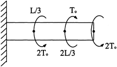
  Figure 4.26

• 4.3 A laboratory test involves “potting” part of the femur in cement and then applying two loads ƒ, each at a distance d from the centerline (cf. Fig. 4.4); this yields a couple or twisting moment T _o  = 2fd. A strain gauge is placed at an angle α on the bone a distance L/2 from the fixed end. Derive a formula for the strain in the gauge that can be related to experimentally measurable quantities. Assume the bone exhibits a LEHI behavior and that it has a cross section at z = L given by inner and outer radii of a and c. Discuss for what such an experiment could be utilized. Discuss why the strain gauge is not applied at length L and angle α = 0.

• 4.4 For a solid shaft of diameter d for z ∊ [0, 2L/3) and diameter nd for z ∊ (2L/3, L], subject to torques T _o at 2L/3 and 2T _o at L, (a) find the value of n such that the maximum shear stress σ _zθ is the same in each segment and (b) find the twist Θ at the free end if n = 1.

• 4.5 Some papillary muscles in the heart (which connect the valves to the endocardium through the chordae) are nearly cylindrical. We wish to perform a torsion test on such a tissue, but measuring the applied torque is difficult because of the small size. Assume that we can use the device in Fig. 4.20, that the wire is made of copper, and that the distance between points A and B is 15 mm. Also assume Θ _A and Θ _B are measurable, their difference being ~90°. If the maximum torque achieved is ~0.5 mN mm, find an appropriate diameter for the wire.

• 4.6 Carter and Beaupré (2001) discuss an interesting finding by Lanyon and Rubin in 1984. It was suggested that the number of cycles of loading per day and the maximum achieved strain both serve as mechanobiological stimuli for bone growth. In particular, they found that bone mass was maintained (i.e., production and removal were balanced) given a strain history of 4 cycles/day at a maximum value of 0.002 or similarly at 100 cycles/day at a maximum value between 0.0005 and 0.001 (assume 0.0008). They suggested that these combined effects can be accounted for via a “daily bone stimulus” parameter ξ that is computed via the following formula

  $$ \xi ={\left(\sum_{\mathrm{day}},{\mathit{\mathrm{n}\upvarepsilon}}^m\right)}^{1/\operatorname{m}} $$

  where n is the number of cycles/day, ε is the maximum strain attained per cycle, and m is an empirically determined material parameter. Given the data listed here, find a value for m.

• 4.7 Based on the results of the previous exercise, determine the number of cycles that one should walk per day if the strain during normal walking is 400 με (i.e., microstrain, where 1 με = 1 × 10⁻⁶). Carter and Beaupré (2001) suggest that 10,000 cycles of walking per day will maintain bone mass. If the normal person advances 3 ft per stride, how far should he/she walk per day to maintain bone mass?

• 4.8 Based on the previous exercise and an assumed Young’s modulus E = 16 GPa and Poisson’s ratio v = 0.325 for bone, compute the axial load necessary to cause a strain of 400 με in the normal adult diaphysial region of the femur. Express your results in terms of percent body weight, assuming a weight of 70 kg. What would the associated axial compressive stress be? Similarly, estimate the load on the femur during running and the associated compressive stress and strain. Based on these values and the previous exercise, if a person advances 4 ft per stride when running, how far should he/she run per day?

• 4.9 If a 17.2-Nm torque induces a maximum shearing strain of 1,132 με at the periosteal surface in the diaphysial region of the femur, what is the associated value of the shearing stress if the shear modulus is 3.3 GPa?

• 4.10 The ratio of the cortical thickness to the outer radius of most human bones is between 0.33 and 0.4. Assume that the cross section of a segment of a long bone is circular and that the periosteal and endosteal radii are 15 mm and 9 mm, respectively. Assume, too, that a 17.2-Nm torque is applied for 10,000 cycles. What is the maximum extensional (principal) strain and, from the equation in Exercise 4.6, what is the value of the daily bone stimulus parameter ξ?

• 4.11 According to Carter and Beaupré (2001), “bone cross-sections that are formed are very dependent on the full history of loading throughout life. In the age range of 30–60 years, the normal bone has a diameter of about 32 mm and a cortical thickness of 5 mm. When the loads are reduced to 40 % of normal at the age of 20, the bone in later adulthood has diameter of about 30 mm and a cortical thickness of about 2 mm. The bone that forms while loads are reduced to 40 % throughout development has an adult diameter of about 22 mm and a thickness of 4 mm.” What are the implications of such observations with regard to space travel, especially a voyage to Mars?

• 4.12 Referring to the previous exercise, note that the strains in adapting bones are generally the same regardless of the applied loads and associated cross-sectional radii. What does this suggest with regard to growth and remodeling?

• 4.13 Carter and Beaupré (2001, p. 81) suggest a phenomenological descriptor of bone growth (actually the rate of increase of the outer radius) of the form, $\dot{r}={\dot{r}}_b+{\dot{r}}_m=c{e}^{-0.9t}+{\dot{r}}_m,$ where $\dot{r}$ is the time rate of change of the radius, having units of microns per day; subscripts b and m denote an intrinsic biological rate and an adaptive mechanobiologic rate, respectively, and t denotes time measured in days. They suggest further that the intrinsic rate becomes relatively small shortly after birth or in early childhood, thus its representation as an exponential decay; that is, they assume that most growth and remodeling occur due to mechanobiologic factors in adolescence and maturity. In simulations, the maximum rate of biological growth was varied from 1 to 20 μm/day. Given these numbers, what would the radius be due to biological growth alone at 6 years of age? Is this value consistent with data on long bones such as the femur?

• 4.14 Referring to Exercise 4.13, Carter and Beaupré (2001, p. 151) note that the mass density of cancellous bone (usually ρ from 570 up to 1,200 kg/m³) is nearly constant from early adolescence to early adulthood. They suggest that this implies that in the absence of bone diseases, the intrinsic biological rate of growth is negligible with respect to the mechanobiological rate during this period. If this is true, what are the implications with regard to the modeling of bone adapatation?

• 4.15 Galileo thought that long bones were hollow because this afforded maximum strength with minimum weight. Discuss this in terms of the ability of a hollow versus a solid cylindrical bone of the same mass to resist a torque; assume the bone is cortical, which has a mass density of ~1,700 kg/m³. Alternatively, is the “hollowness” of a long bone consistent with a stress- or strain-based growth model wherein a maximum compressive strain of 1,000 με is homeostatic—assume that the bone is either subjected to a torque alone or to a combined torque and axial load wherein the stresses due to torsion exceed those due to axial loading?

• 4.16 A long bone is subjected to a torsion test. Assume that the inner diameter is 0.375 in. and the outer diameter is 1.25 in., both for a circular cross section. If E = 16 GPa and v = 0.325, find the largest torque that can be applied prior to yield, where σ _yield = 1.25 ksi (i.e., a maximum normal stress).

• 4.17 A solid circular cylinder 10 cm long and 2 cm in outer radius behaves as a LEHI material with G = 10 GPa. If the twisting moment (torque) applied at the free end is 3 kNm, show that J = 25.13 × 10⁻⁸ m⁴, Θ = 6.84° at the free end, σ _zθ (r = c) = 238.76 MPa, and 2ε _zθ (r = c) = 0.02388. Assume one end is fixed.

• 4.18 A rectangular bar 2 × 2 × 20 cm in dimension is subjected to an axial force (uniform) of 4 × 10⁶ N. Assuming E = 100 GPa and v = 0.30, find σ _xx , ε _xx , ε _yy  = ε _zz , and the deformed dimensions (assuming homogenous strains).

• 4.19 A human femur is mounted in a torsion testing device and loaded to failure. Assuming that one end is fixed and the other rotated, failure (fracture) occurs when T = 180 Nm and Θ(L) = 20°. Assume that L = 37 cm and that the failure occurs at 25 cm from the fixed end, where the inner and outer radii are 7 mm and 13 mm, respectively. Find the value of the shear stress at which fracture occurs; estimate the shear modulus G. Finally, note that “torsional fractures are usually initiated at regions of the bones where the cross-sections are the smallest. Some particularly weak sections of human bones are the upper and lower thirds of the humerus, femur, and fibula; the upper third of the radius; and the lower fourth of the ulna and tibia” (Özkaya and Nordin 1999).

• 4.20 A rectangular aluminum bar (~1.5 × 2.1 cm in cross section) and a circular steel rod (~1 cm in radius) are each subjected to an axial force of 20 kN. Assuming that both are 30 cm long in their unloaded configuration, find (a) the stress in each, (b) the extensional strain in each, and (c) the amount of lengthening in each. Let E = 70 GPa for aluminum and 200 GPa for steel.

• 4.21 A brittle behavior is characterized by an abrupt fracture soon after the elastic limit is exceeded. In contrast, a ductile behavior is characterized by a plastic behavior, including strain hardening, following yield. Recall Fig. 2.25. We know that yield and the subsequent plastic behavior are governed by shear stresses, which cause atoms to “slip” past one another irreversibly. Hence, it is important to compute the maximum shear stress. Although a shear stress at which a material yields is easy to determine in a torsion test, tensile tests are more common. Recall from Chap. 2, therefore, that the maximum shear stress in a 1-D tension test $\left({\sigma}_{xx}={\sigma}_1,\;{\sigma}_{yy}=0,\;{\sigma}_{xy}=0\right)$ is

  $$ {\sigma}_{xy}^{\prime}\Big){}_{\max }=\sqrt{{\left(\frac{\sigma_1-0}{2}\right)}^2+{0}^2}=\frac{\sigma_1}{2}. $$

  This value of σ ₁ at yield is called σ _y , the yield stress. Hence, a yield criterion in uniaxial tension is as follows: If ∣σ _xx ∣ ≤ σ _y , then the material has not yielded. In multiaxial states of stress, more general yield criteria are needed. Two common yield theories are the Tresca yield condition and the von Mises yield conditions. Research these two yield theories and submit a two-page summary.

References

Alberts B, Johnson A, Lewis J, Raff M, Roberts K, Walter P (2002) Molecular biology of the cell. Garland, New York, NY
Carter DR, Beaupré GS (2001) Skeletal function and form: mechanobiology of skeletal development, aging, and regeneration. Cambridge University Press, Cambridge
Fawcett DW (1986) Bloom and Fawcett: a textbook of histology, 11th edn. W.B. Saunders, Philadelphia, PA
Humphrey JD (2001) Stress, strain and mechanotransduction in cells. J Biomech Eng 123:638–641
Humphrey JD (2002) Cardiovascular solid mechanics: cells, tissues, and organs. Springer, New York, NY
Özkaya N, Nordin M (1999) Fundamentals of biomechanics: equilibrium, motion, and deformation. Springer, New York, NY
Rubin CT, Lanyon L (1985) Regulation of bone mass by mechanical loading: the effect of peak strain magnitude. Calcif Tissue Int 37:441–447
Sten-Knudsen O (1953) Torsional elasticity of the isolated cross striated muscle fibre. Acta Physiol Scand 28:7–240
Wolff J (1986) The law of bone remodeling. Springer, Berlin
Author information
Authors and Affiliations