Synchronization: Why and How to Avoid It

Abstract

Let us underscore this up front: if you don’t need to use the synchronization features described in this chapter, so much the better. Here, we cover synchronization mechanisms and alternatives to achieve mutual exclusion. “Synchronization” and “exclusion” should have quite a negative connotation for parallel programmers caring about performance. These are operations that we want to avoid because they cost time and, in some cases, processor resources and energy. If we can rethink our data structures and algorithm so that it does not require synchronization nor mutual exclusion, this is great! Unfortunately, in many cases, it is impossible to avoid synchronization operations, and if this is your case today, keep reading! An additional take-home message that we get from this chapter is that careful rethinking of our algorithm can usually result in a cleaner implementation that does not abuse synchronization. We illustrate this process of rethinking an algorithm by parallelizing a simple code following first a naïve approach that resorts to mutexes, evolve it to exploit atomic operations, and then further reduce the synchronization between threads thanks to privatization and reduction techniques. To this final end, we show how to leverage thread local storage (TLS) as a way to avoid highly contended mutual exclusion overhead. In the sequel, we assume you are, to some extent, familiarized with the concepts of “lock,” “shared mutable state,” “mutual exclusion,” “thread safety,” “data race,” and other synchronization-related issues. If not, a gentle introduction to them is provided in the Preface of this book.

Let us underscore this up front: if you don’t need to use the synchronization features described in this chapter, so much the better. Here, we cover synchronization mechanisms and alternatives to achieve mutual exclusion. “Synchronization” and “exclusion” should have quite a negative connotation for parallel programmers caring about performance. These are operations that we want to avoid because they cost time and, in some cases, processor resources and energy. If we can rethink our data structures and algorithm so that it does not require synchronization nor mutual exclusion, this is great! Unfortunately, in many cases, it is impossible to avoid synchronization operations, and if this is your case today, keep reading! An additional take-home message that we get from this chapter is that careful rethinking of our algorithm can usually result in a cleaner implementation that does not abuse synchronization. We illustrate this process of rethinking an algorithm by parallelizing a simple code following first a naïve approach that resorts to mutexes, evolve it to exploit atomic operations, and then further reduce the synchronization between threads thanks to privatization and reduction techniques. In the latter of these, we show how to leverage thread local storage (TLS) as a way to avoid highly contended mutual exclusion overhead. In this chapter, we assume you are, to some extent, familiarized with the concepts of “lock,” “shared mutable state,” “mutual exclusion,” “thread safety,” “data race,” and other synchronization-related issues. If not, a gentle introduction to them is provided in the Preface of this book.

A Running Example: Histogram of an Image

Let’s us start with a simple example that can be implemented with different kinds of mutual exclusion (mutex) objects, atomics, or even by avoiding most of the synchronization operations altogether. We will describe all these possible implementations with their pros and cons, and use them to illustrate the use of mutexes, locks, atomic variables, and thread local storage.

There are different kinds of histograms, but an image histogram is probably the most widely used, especially in image and video devices and image processing tools. For example, in almost all photo editing applications, we can easily find a palette that shows the histogram of any of our pictures, as we see in Figure 5-1.

Figure 5-1.

Grayscale picture (of Ronda, Málaga) and its corresponding image histogram

For the sake of simplicity, we will assume grayscale images. In this case, the histogram represents the number of pixels (y-axis) with each possible brightness value (x-axis). If image pixels are represented as bytes, then only 256 tones or brightness values are possible, with zero being the darkest tone and 255 the lightest tone. In Figure 5-1, we can see that the most frequent tone in the picture is a dark one: out of the 5 Mpixels, more than 70 thousand have the tone 30 as we see at the spike around x=30. Photographers and image professionals rely on histograms as an aid to quickly see the pixel tone distribution and identify whether or not image information is hidden in any blacked out, or saturated, regions of the picture.

In Figure 5-2, we illustrate the histogram computation for a 4×4 image where the pixels can only have eight different tones from 0 to 7. The bidimensional image is usually represented as a unidimensional vector that stores the 16 pixels following a row-major order. Since there are only eight different tones, the histogram only needs eight elements, with indices from 0 to 7. The elements of the histogram vector are sometime called “bins” where we “classify” and then count the pixels of each tone. Figure 5-2 shows the histogram, hist, corresponding to that particular image. The “4” we see stored in bin number one is the result of counting the four pixels in the image with tone 1. Therefore, the basic operation to update the value of the bins while traversing the image is hist[<tone>]++.

Figure 5-2.

Computing the histogram, hist, from an image with 16 pixels (each value of the image corresponds to the pixel tone)

From an algorithmic point of view, a histogram is represented as an array of integers with enough elements to account for all possible tone levels. Assuming the image is an array of bytes, there are now 256 possible tones; thus, the histogram requires 256 elements or bins. The sequential code that computes the histogram of such an image is presented in Figure 5-3.

Figure 5-3.

Code listing with the sequential implementation of the image histogram computation. The relevant statements are highlighted inside a box.

If you already understand everything in the previous code listing, you will probably want to skip the rest of this section. This code first declares the vector image of size n (say one million for a Megapixel image) and, after initializing the random number generator, it populates the image vector with random numbers in the range [0,255] of type uint8_t. For this, we use a Mersenne_twister_engine, mte, which generates random numbers uniformly distributed in the range [0, num_bins) and inserts them into the image vector. Next, the hist vector is constructed with num_bins positions (initialized to zero by default). Note that we declared an empty vector image for which we later reserved n integers instead of constructing image(n). That way we avoid traversing the vector first to initialize it with zeros and once again to insert the random numbers.

The actual histogram computation could have been written in C using a more traditional approach:

for (int i = 0; i < N; ++i) hist[image[i]]++;

which counts in each bin of the histogram vector the number of pixels of every tonal value. However, in the example of Figure 5-3, we fancied showing you a C++ alternative that uses the STL for_each algorithm and may be more natural for C++ programmers. Using the for_each STL approach, each actual element of the image vector (a tone of type uint8_t) is passed to the lambda expression, which increments the bin associated with the tone. For the sake of expediency, we rely on the tbb::tick_count class in order to account for the number of seconds required in the histogram computation. The member functions now and seconds are self-explanatory, so we do not include further explanation here.

An Unsafe Parallel Implementation

The first naïve attempt to parallelize the histogram computation consists on using a tbb: :parallel_for as shown in Figure 5-4.

Figure 5-4.

Code listing with the unsafe parallel implementation of the image histogram computation

In order to be able to compare the histogram resulting from the sequential implementation of Figure 5-3, and the result of the parallel execution, we declare a new histogram vector hist_p. Next, the crazy idea here is to traverse all the pixels in parallel… why not? Aren’t they independent pixels? To that end, we rely on the parallel_for template that was covered in Chapter 2 to have different threads traverse different chunks of the iteration space and, therefore, read different chunks of the image. However, this is not going to work: the comparison of vectors hist and hist_p (yes, hist!=hist_p does the right thing in C++), at the end of Figure 5-4, reveals that the two vectors are different:

   c++ -std=c++11 -O2 -o fig_5_4 fig_5_4.cpp -ltbb    ./fig_5_4    Serial: 0.606273, Parallel: 6.71982, Speed-up: 0.0902216    Parallel computation failed!!

A problem arises because, in the parallel implementation, different threads are likely to increment the same shared bin at the same time. In other words, our code is not thread-safe (or unsafe). More formally, as it is, our parallel unsafe code exhibits “undefined behavior” which also means that our code is not correct. In Figure 5-5 we illustrate the problem supposing that there are two threads, A and B, running on cores 0 and 1, each one processing half of the pixels. Since there is a pixel with brightness 1 in the image chunk assigned to thread A, it will execute hist_p[1]++. Thread B also reads a pixel with the same brightness and will also execute hist_p[1]++. If both increments coincide in time, one executed on core 0 and the other on core 1, it is highly likely that we miss an increment.

Figure 5-5.

Unsafe parallel update of the shared histogram vector

This happens because the increment operation is not atomic (or indivisible), but on the contrary it usually consists of three assembly level operations: load the variable from memory into a register, increment the register, and store the register back into memory.¹ Using a more formal jargon, this kind of operation is known as a Read-Modify-Write or RMW operation. Having concurrent writes to a shared variable is formally known as shared mutable state. In Figure 5-6, we illustrate a possible sequence of machine instructions corresponding to the C++ instruction hist_p[1]++.

Figure 5-6.

Unsafe update of a shared variable or shared mutable state

If at the time of executing these two increments we have already found one previous pixel with brightness 1, hist_p[1] contains a value of one. This value could be read and stored in private registers by both threads which will end up writing two in this bin instead of three, which is the correct number of pixels with brightness 1 that have been encountered thus far. This example is somehow oversimplified, not taking into account caches and cache coherence, but serve us to illustrate the data race issue. A more elaborated example is included in the Preface (see Figures P-15 and P-16).

We might think that this series of unfortunate events are unlikely to happen, or even if they happen, that slightly different result will be acceptable when running the parallel version of the algorithm. Is not the reward a faster execution? Not quite: as we saw in the previous page, our unsafe parallel implementation is ~10× slower than the sequential one (running with four threads on a quad-core processor and with n equal to one thousand million pixels). The culprit is the cache coherency protocol that was introduced in the Preface (see “Locality and the Revenge of the Caches” section in the Preface). In the serial execution, the histogram vector is likely to be fully cached in the L1 cache of the core running the code. Since there are a million pixels, there will be a million of increments in the histogram vector, most of them served at cache speed.

Note

On most Intel processors, a cache line can hold 16 integers (64 bytes). The histogram vector with 256 integers will need just 16 cache lines if the vector is adequately aligned. Therefore, after 16 cache misses (or much less if prefetching is exercised), all histogram bins are cached and each one accessed in only around three cycles (that’s very fast!) in the serial implementation (assuming a large enough L1 cache and that the histogram cache lines are never evicted by other data).

On the other hand, in the parallel implementation, all threads will fight to cache the bins in per-core private caches, but when one thread writes in one bin on one core, the cache coherence protocol invalidates the 16 bins that fit in the corresponding cache line in all the other cores. This invalidation causes the subsequent accesses to the invalidated cache lines to cost an order of magnitude more time than the much desired L1 access time. The net effect of this ping-pong mutual invalidation is that the threads of the parallel implementation end up incrementing un-cached bins, whereas the single thread of the serial implementation almost always increments cached bins. Remember once again that the one-megapixel image requires one million increments in the histogram vector, so we want to create an increment implementation that is as fast as possible. In this parallel implementation of the histogram computation, we find both false sharing (e.g., when thread A increments hist_p[0] and thread B increments hist_p[15], due to both bins land in the same cache line) and true sharing (when both threads, A and B, increment hist_p[i]). We will deal with false and true sharing in subsequent sections.

A First Safe Parallel Implementation: Coarse-Grained Locking

Let’s first solve the problem of the parallel access to a shared data structure. We need a mechanism that prevents other threads from reading and writing in a shared variable when a different thread is already in the process of writing the same variable. In more layman terms, we want a fitting room where a single person can enter, see how the clothes fit, and then leaves the fitting room for the next person in the queue. Figure 5-7 illustrates that a closed door on the fitting room excludes others. In parallel programming, the fitting room door is called a mutex , when a person enters the fitting room he acquires and holds a lock on the mutex by closing and locking the door, and when the person leaves they release the lock by leaving the door open and unlocked. In more formal terms, a mutex is an object used to provide mutual exclusion in the execution of a protected region of code. This region of code that needs to be protected with mutual exclusion is usually known as a “critical section.” The fitting room example also illustrates the concept of contention, a state where the resource (a fitting room) is wanted by more than one person at a time, as we can see in Figure 5-7(c). Since the fitting room can be occupied just by a single person at a time, the use of the fitting room is “serialized.” Similarly, anything protected by a mutex can reduce the performance of a program, first due to the extra overhead introduced by managing the mutex object, and second and more importantly because the contention and serialization it can elicit. A key reason we want to reduce synchronization as much as possible is to avoid contention and serialization which in turns limits scaling in parallel programs.

Figure 5-7.

Closing a door on a fitting room excludes others

In this section, we focus on the TBB mutex classes and related mechanisms for synchronization. While TBB predates C++11, it is worth noting that C++11 did standardize support for a mutex class, although it is not as customizable as the ones in the TBB library. In TBB, the simplest mutex is the spin_mutex that can be used after including tbb/spin_mutex.h or the all-inclusive tbb.h header file. With this new tool in our hands, we can implement a safe parallel version of the image histogram computation as we can see in Figure 5-8.

Figure 5-8.

Code listing with our first safe parallel implementation of the image histogram computation that uses coarse-grained locking

The object my_lock that acquires a lock on my_mutex, when it is created automatically unlocks (or releases) the lock in the object destructor, which is called when leaving the object scope. It is therefore advisable to enclose the protected regions with additional braces, {}, to keep the lifetime of the lock as short as possible, so that the other waiting threads can take their turn as soon as possible.

Note

If in the code of Figure 5-8 we forget to put a name to the lock object, for example:

// was my_lock{my_mutex} my_mutex_t::scoped_lock {my_mutex};

the code compiles without warning, but the scope of the scoped_lock ends at the semicolon. Without the name of the object (my_lock), we are constructing an anonymous/unnamed object of the scoped_lock class, and its lifetime ends at the semicolon because no named object outlives the definition. This is not useful, and the critical section is not protected with mutual exclusion.

A more explicit, but not recommended, alternative of writing the code of Figure 5-8 is presented in Figure 5-9.

Figure 5-9

A discouraged alternative for acquiring a lock on a mutex

C++ pundits favor the alternative of Figure 5-8, known as “Resource Acquisition Is Initialization,” RAII, because it frees us from remembering to release the lock. More importantly, using the RAII version, the lock object destructor, where the lock is released, is also called in case of an exception so that we avoid leaving the lock acquired due to the exception. If in the version of Figure 5-9 an exception is thrown before the my_lock.release() member function is called, the lock is also released anyway, because the destructor is invoked and there, the lock is released. If a lock leaves its scope but was previously released with the release() member function, then the destructor does nothing.

Back to our code of Figure 5-8, you are probably wondering, “but wait, haven’t we serialized our parallel code with a coarse-grained lock?” Yes, you are right! As we can see in Figure 5-10, each thread that wants to process its chunk of the image first tries to acquire the lock on the mutex, but only one will succeed and the rest will impatiently wait for the lock to be released. Not until the thread holding the lock releases it, can a different thread execute the protected code. Therefore, the parallel_for ends up being executed serially! The good news is that now, there are no concurrent increments of the histogram bins and the result is finally correct. Yeah!

Figure 5-10

Thread A holds the coarse-grained lock to increment bin number one, while thread B waits because the whole histogram vector is locked

Actually, if we compile and run our new version, what we get is a parallel execution a little bit slower than the sequential one:

   c++ -std=c++11 -O2 -o fig_5_8 fig_5_8.cpp -ltbb    ./fig_5_8    Serial: 0.61068, Parallel: 0.611667, Speed-up: 0.99838

This approach is called coarse-grained locking because we are protecting a coarse-grained data structure (actually the whole data structure – the histogram vector – in this case). We could partition the vector in several sections and protect each section with its own lock. That way, we would increase the concurrency level (different threads accessing different sections can proceed in parallel), but we would have increased the complexity of the code and the memory required for each of the mutex objects.

A word of caution is in order! Figure 5-11 shows a common mistake of parallel programming newbies.

Figure 5-11

Common mistake made by parallel programming newbies

This code compiles without errors nor warnings, so what is wrong with it? Back to our fitting-room example, our intention was to avoid several people entering in the fitting-room at the same time. In the previous code, my_mutex is defined inside the parallel section, and there will be a mutex object per task, each one locking its own mutex, which does not prevent concurrent access to the critical section. As we can see in Figure 5-12, the newbie code essentially has a separate door for each person into the same fitting room! That is not what we want! The solution is to declare my_mutex once (as we did in Figure 5-8) so that all accesses have to enter the fitting room through the same door.

Figure 5-12

A fitting room with more than one door

Before tackling a fine-grained locking alternative, let’s discuss two aspects that deserve a comment. First, the execution time of the “parallelized-then-serialized” code of Figure 5-8 is greater than the time needed by the serial implementation. This is due to the “parallelization-then-serialization” overhead, but also due to a poorer exploitation of the caches. Of course, there is no false sharing nor true sharing, because in our serialized implementation there is no “sharing” whatsoever! Or is there? In the serial implementation, only one thread accesses a cached histogram vector. In the coarse-grained implementation, when one thread processes its chunk of the image, it will cache the histogram in the cache of the core where the thread is running. When the next thread in the queue can finally process its own chunk, it may need to cache the histogram in a different cache (if the thread is running on a different core). The threads are still sharing the histogram vector, and more cache misses will likely occur with the proposed implementation than with the serial one.

The second aspect that we want to mention is the possibility of configuring the mutex behavior by choosing one of the possible mutex flavors that are shown in Figure 5-13. It is therefore recommended to use

using my_mutex_t = <mutex_flavor>

or the equivalent C-ish alternative

typedef <mutex_flavor> my_mutex_t;

and then use my_mutex_t onward. That way, we can easily change the mutex flavor in a single program line and experimentally evaluate easily which flavor suits us best. It may be necessary to also include a different header file, as indicated in Figure 5-13, or use the all-inclusive tbb.h .

Figure 5-13

Different mutex flavors and their properties

Mutex Flavors

In order to understand the different flavors of mutex, we have to first describe the properties that we use to classify them:

• Scalable mutexes do not consume excessive core cycles nor memory bandwidth while waiting to have their turn. The motivation is that a waiting thread should avoid consuming the hardware resources that may be needed by other nonwaiting threads.

• Fair mutexes use a FIFO policy for the threads to take their turn.

• Recursive mutexes allow that a thread already holding a lock on a mutex can acquire another lock on the same mutex. Rethinking your code to avoid mutexes is great, doing it to avoid recursive mutexes is almost a must! Then, why does TBB provide them? There may be corner cases in which recursive mutexes are unavoidable. They may also come in handy when we can’t be bothered or have no time to rethink a more efficient solution.

In the table in Figure 5-13, we also include the size of the mutex object and the behavior of the thread if it has to wait for a long time to get a lock on the mutex. With regard to the last point, when a thread is waiting its turn it can busy-wait, block, or yield. A thread that blocks will be changed to the blocked state so that the only resource required by the thread is the memory that keeps its sleeping state. When the thread can finally acquire the lock, it wakes up and moves back to the ready state where all the ready threads wait for their next turn. The OS scheduler assigns time slices to the ready threads that are waiting in a ready-state queue. A thread that yields while waiting its turn to hold a lock is kept in the ready state. When the thread reaches the top of the ready-state queue, it is dispatched to run, but if the mutex is still locked by other thread, it again gives away its time slice (it has nothing else to do!) and goes back to the ready-state queue.

Note

Note that in this process there may be two queues involved: (i) the ready-state queue managed by the OS scheduler, where ready threads are waiting, not necessarily in FIFO order, to be dispatched to an idle core and become running threads, and (ii) the mutex queue managed by the OS or by the mutex library in user space, where threads wait their turn to acquire a lock on a queueing mutex.

If the core is not oversubscribed (there is only one thread running in this core), a thread that yields because the mutex is still locked will be the only one in the ready-state queue and be dispatched right away. In this case, the yield mechanism is virtually equivalent to a busy-wait.

Now that we understand the different properties that can characterize the implementation of a mutex, let’s delve into the particular mutex flavors that TBB offers.

mutex and recursive_mutex are TBB wrappers around the OS-provided mutex mechanism. Instead of the “native” mutex, we use TBB wrappers because they add exception-safe and identical interfaces to the other TBB mutexes. These mutexes block on long waits, so they waste fewer cycles, but they occupy more space and have a longer response time when the mutex becomes available.

spin_mutex , on the contrary, never blocks. It spins busy-waiting in the user space while waiting to hold a lock on a mutex. The waiting thread will yield after a number of tries to acquire the loop, but if the core is not oversubscribed, this thread keeps the core wasting cycles and power. On the other hand, once the mutex is released, the response time to acquire it is the fastest possible (no need to wake up and wait to be dispatched to run). This mutex is not fair, so no matter for how long a thread has been waiting its turn, a quicker thread can overtake it and acquire the lock if it is the first to find the mutex unlocked. A free-for-all prevails in this case, and in extreme situations, a weak thread can starve, never getting the lock. Nonetheless, this is the recommended mutex flavor under light contention situations because it can be the fastest one.

queueing_mutex is the scalable and fair version of the spin_mutex. It still spins, busy-waiting in user space, but threads waiting on that mutex will acquire the lock in FIFO order, so starvation is not possible.

speculative_spin_mutex is built on top of Hardware Transactional Memory (HTM) that is available in some processors. The HTM philosophy is to be optimistic! HTM lets all threads enter a critical section at the same time hoping that there will be no shared memory conflicts! But what if there are? In this case, the hardware detects the conflict and rolls back the execution of one of the conflicting threads, which has to retry the execution of the critical section. In the coarse-grained implementation shown in Figure 5-8, we could add this simple line:

using my_mutex_t = speculative_spin_mutex;

and then, the parallel_for that traverses the image becomes parallel once again. Now, all threads are allowed to enter the critical section (to update the bins of the histogram for a given chunk of the image), but only if there is an actual conflict updating one of the bins, one of the conflicting threads has to retry the execution. For this to work efficiently, the protected critical section has to be small enough so that conflicts and retries are rare, which is not the case in the code of Figure 5-8.

spin_rw_mutex, queueing_rw_mutex, and speculative_spin_rw_mutex are the Reader-Writer mutex counterparts of the previously covered flavors. These implementations allow multiple readers to read a shared variable at the same time. The lock object constructor has a second argument, a boolean, that we set to false if we will only read (not write) inside the critical section:

If for any reason, a reader lock has to be promoted to a writer lock, TBB provides an upgrade_to_writer() member function that can be used as follows:

which returns true if the my_lock is successfully upgraded to a writer lock without releasing the lock, or false otherwise.

Finally, we have null_mutex and null_rw_mutex that are just dummy objects that do nothing. So, what’s the point? Well, we can find these mutexes useful if we pass a mutex object to a function template that may or may not need a real mutex. In case the function does not really need the mutex, just pass the dummy flavor.

A Second Safe Parallel Implementation: Fine-Grained Locking

Now that we know a lot about the different flavors of mutexes, let’s think about an alternative implementation of the coarse-grained locking one in Figure 5-8. One alternative is to declare a mutex for every bin of the histogram so that instead of locking the whole data structure with a single lock, we only protect the single memory position that we are actually incrementing. To do that, we need a vector of mutexes, fine_m, as the one shown in Figure 5-14.

Figure 5-14

Code listing with a second safe parallel implementation of the image histogram computation that uses fine-grained locking

As we see in the lambda used inside the parallel_for, when a thread needs to increment the bin hist_p[tone], it will acquire the lock on fine_m[tone], preventing other threads from touching the same bin. Essentially “you can update other bins, but not this particular one.” This is illustrated in Figure 5-15 where thread A and thread B are updating in parallel different bins of the histogram vector.

Figure 5-15

Thanks to fine-grained locking, we exploit more parallelism

However, from a performance standpoint, this alternative is not really an optimal one (actually it is the slowest alternative up to now):

c++ -std=c++11 -O2 -o fig_5_14 fig_5_14.cpp -ltbb ./fig_5_14 Serial: 0.59297, Parallel: 26.9251, Speed-up: 0.0220229

Now we need not only the histogram array but also an array of mutex objects of the same length. This means a larger memory requirement, and moreover, more data that will be cached and that will suffer from false sharing and true sharing . Bummer!

In addition to the lock inherent overhead, locks are at the root of two additional problems: convoying and deadlock. Let’s cover first “convoying.” This name comes from the mental image of all threads convoying one after the other at the lower speed of the first one. We need an example to better illustrate this situation, as the one depicted in Figure 5-16. Let’s suppose we have threads 1, 2, 3, and 4 executing on the same core the same code, where there is a critical section protected by a spin mutex A. If these threads hold the lock at different times, they run happily without contention (situation 1). But it may happen that thread 1 runs out of its time slice before releasing the lock, which sends A to the end of the ready-state queue (situation 2).

Figure 5-16

Convoying in the case of oversubscription (a single core running four threads, all of them wanting the same mutex A)

Threads 2, 3, and 4 will now get their corresponding time slices, but they cannot acquire the lock because 1 is still the owner (situation 3). This means that 2, 3, and 4 can now yield or spin, but in any case, they are stuck behind a big truck in first gear. When 1 is dispatched again, it will release the lock A (situation 4). Now 2, 3, and 4 are all poised to fight for the lock, with only one succeeding and the others waiting again. This situation is recurrent, especially if now threads 2, 3, and 4 need more than a time slice to run their protected critical section. Moreover, threads 2, 3, and 4 are now inadvertently coordinated, all running in step the same region of the code, which leads to a higher probability of contention on the mutex! Note that convoying is especially acute when the cores are oversubscribed (as in this example where four threads compete to run on a single core) which also reinforces our recommendation to avoid oversubscription.

An additional well-known problem arising from locks is “deadlock.” Figure 5-17(a) shows a nightmare provoking situation in which nobody can make progress even when there are available resources (empty lines that no car can use). This is deadlock in real life, but get this image out of your head (if you can!) and come back to our virtual world of parallel programming. If we have a set of N threads that are holding a lock and also waiting to acquire a lock already held by any other thread in the set, our N threads are deadlocked. An example with only two threads is presented in Figure 5-17(b): thread 1 holds a lock on mutex A and is waiting to acquire a lock on mutex B, but thread 2 is already holding the lock on mutex B and waiting to acquire the lock on mutex A. Clearly, no thread will progress, forever doomed in a deadly embrace! We can avoid this unfortunate situation by not requiring the acquisition of a different mutex if the thread is already holding one. Or at least, by having all threads always acquire the locks in the same order.

Figure 5-17

Deadlock situations

We can inadvertently provoke deadlock if a thread already holding a lock calls a function that also acquires a different lock. The recommendation is to eschew calling a function while holding a lock if we don’t know what the function does (usually advised as don’t call other people’s code while holding a lock). Alternatively, we should carefully check that the chain of subsequent functions call won’t induce deadlock. Ah! and we can also avoid locks whenever possible!

Although convoying and deadlock are not really hitting our histogram implementation, they should have helped to convince us that locks often bring more problems than they solve and that they are not the best alternative to get high parallel performance. Only when the probability of contention is low and the time to execute the critical section is minimal are locks a tolerable choice. In these cases, a basic spin_lock or speculative_spin_lock can yield some speedup. But in any other cases, the scalability of a lock based algorithm is seriously compromised and the best advice is to think out of the box and devise a new implementation that does not require a mutex altogether. But, can we get fine-grained synchronization without relying on several mutex objects, so that we avoid the corresponding overheads and potential problems?

A Third Safe Parallel Implementation: Atomics

Fortunately, there is a less expensive mechanism to which we can resort to get rid of mutexes and locks in many cases. We can use atomic variables to perform atomic operations. As was illustrated in Figure 5-6, the increment operation is not atomic but divisible into three smaller operations (load, increment, and store). However, if we declare an atomic variable and do the following:

the increment of the atomic variable is an atomic operation. This means that any other thread accessing the value of counter will “see” the operation as if the increment is done in a single step (not as three smaller operations, but as a single one). This is, any other “sharp-eyed” thread will either observe the operation completed or not, but it will never observe the increment half-complete.

Atomic operations do not suffer from convoying or deadlock² and are faster than mutual exclusion alternatives. However, not all operations can be executed atomically, and those that can, are not applicable to all data types. More precisely, atomic<T> supports atomic operations when T is an integral, enumeration, or pointer data type. The atomic operations supported on a variable x of such a type atomic<T> are listed in Figure 5-18.

Figure 5-18

Fundamental operations on atomic variables

With these five operations, a good deal of derived operations can be implemented. For example, x++, x--, x+=..., and x-=... are all derived from x.fetch_and_add().

Note

As we have already mentioned in previous chapters, C++ also incorporated threading and synchronization features, starting at C++11. TBB included these features before they were accepted in the C++ standard. Although starting at C++11, std::mutex and std::atomic, among others, are available, TBB still provides some overlapping functionalities in its tbb::mutex and tbb::atomic classes, mainly for compatibility with previously developed TBB-based applications. We can use both flavors in the same code without problem, and it is up to us to decide if one or the other is preferable for a given situation. Regarding std::atomic, some extra performance, w.r.t. tbb::atomic, can be wheedle out if used to develop lock-free algorithms and data structures on “weakly-ordered” architectures (as ARM or PowerPC; in contrast, Intel CPUs feature a strongly-ordered memory-model). In the last section of this chapter, “For More Information,” we recommend further readings related to memory consistency and C++ concurrency model where this topic is thoroughly covered. For our purpose here, suffice it to say that fetch_and_store, fetch_and_add, and compare_and_swap adhere by default to the sequential consistency (memory_order_seq_cst in C++ jargon), which can prevent some out-of-order execution and therefore cost a tiny amount of extra time. To account for that, TBB also offers release and acquire semantic: acquire by default in atomic read (...=x); and release by default in atomic write (x=...). The desired semantic can also be specified using a template argument, for example, x.fetch_and_add<release> enforces only the release memory order. In C++11, other more relaxed memory orders are also allowed (memory_order_relaxed and memory_order_consume) which in particular cases and architectures can allow for more latitude on the order of reads and writes and squeeze a small amount of extra performance. Should we want to work closer to the metal for the ultimate performance, even knowing the extra coding and debugging burden, then C++11 lower level features are there for us, and yet we can combine them with our higher-level abstractions provided by TBB.

Another useful idiom based on atomics is the one already used in the wavefront example presented in Figure 2-23 (Chapter 2). Having an atomic integer refCount initialized to “y” and several threads executing this code:

will result in only the y-th thread executing the previous line entering in the “body.”

Of these five fundamental operations, compare_and_swap (CAS) can be considered as the mother of all atomic read-modify-write, RMW, operations. This is because all atomic RMW operations can be implemented on top of a CAS operation.

Note

Just in case you need to protect a small critical section and you are already convinced of dodging locks at any rate, let’s dip our toes into the details of the CAS operation a little bit. Say that our code requires to atomically multiply a shared integer variable, v, by 3 (don’t ask us why! we have our reasons!). We are aiming for a lock-free solution, though we know that multiplication is not included as one of the atomic operations. Here is where CAS comes in. First thing is to declare v as an atomic variable:

tbb::atomic<uint_32_t> v;

so now we can call v.compare_and_swap(new_v, old_v) which atomically does

This is, if and only if v is equal to old_v, we can update v with the new value. In any case, we return ov (the shared v used in the “==” comparison). Now, the trick to implement our “times 3” atomic multiplication is to code what is dubbed CAS loop:

Our new fetch_and_triple is thread-safe (can be safely called by several threads at the same time) even when it is called passing the same shared atomic variable. This function is basically a do-while loop in which we first take a snapshot of the shared variable (which is key to later compare if other thread has managed to modify it). Then, atomically, if no other thread has changed v (v==old_v), we do update it (v=old_v*3) and return v. Since in this case v == old_v (again: no other thread has changed v), we leave the do-while loop and return from the function with our shared v successfully updated.

However, after taking the snapshot, it is possible that other thread updates v. In this case, v!=old_v which implies that (i) we do not update v and (ii) we stay in the do-while loop hoping that lady luck will smile on us next time (when no other greedy thread dares to touch our v in the interim between the moment we take the snapshot and we succeed updating v). Figure 5-19 illustrates how v is always updated either by thread 1 or thread 2. It is possible that one of the threads has to retry (as thread 2 that ends up writing 81 when initially it was about to write 27) one or more times, but this shouldn’t be a big deal in well-devised scenarios.

The two caveats of this strategy are (i) it scales badly and (ii) it may suffer from the “ABA problem” (there is background on the classic ABA problem in Chapter 6 on page 201). Regarding the first one, consider P threads contending for the same atomic, only one succeeds with P-1 retrying, then another succeeds with P-2 retrying, then P-3 retrying, and so on, resulting in a quadratic work. This problem can be ameliorated resorting to an “exponential back off” strategy that multiplicatively reduces the rate of consecutive retries to reduce contention. On the other hand, the ABA problem happens when, in the interim time (between the moment we take the snapshot and we succeed updating v), a different thread changes v from value A to value B and back to value A. Our CAS loop can succeed without noticing the intervening thread, which can be problematic. Double check you understand this problem and its consequences if you need to resort to a CAS loop in your developments.

Figure 5-19

Two threads concurrently calling to our fetch_and_triple atomic function implemented on top of a CAS loop

But now it is time to get back to our running example. A re-implementation of the histogram computation can now be expressed with the help of atomics as shown in Figure 5-20.

Figure 5-20

Code listing with a third safe parallel implementation of the image histogram computation that uses atomic variables

In this implementation, we get rid of the mutex objects and locks and declare the vector so that each bin is a tbb::atomic<int> (initialized to 0 by default). Then, in the lambda, it is safe to increment the bins in parallel. The net result is that we get parallel increments of the histogram vector, as with the fine-grained locking strategy, but at a lower cost both in terms of mutex management and mutex storage.

However, performance wise, the previous implementation is still way too slow:

c++ -std=c++11 -O2 -o fig_5_20 fig_5_20.cpp -ltbb ./fig_5_20 Serial: 0.614786, Parallel: 7.90455, Speed-up: 0.0710006

In addition to the atomic increment overhead, false sharing and true sharing are issues that we have not addressed yet. False sharing is tackled in Chapter 7 by leveraging aligned allocators and padding techniques. False sharing is a frequent showstopper that hampers parallel performance, so we highly encourage you to read in Chapter 7 the recommended techniques to avoid it.

Great, assuming that we have fixed the false sharing problem, what about the true sharing one? Two different threads will eventually increment the same bin, which will be ping-pong from one cache to other. We need a better idea to solve this one!

A Better Parallel Implementation: Privatization and Reduction

The real problem posed by the histogram reduction is that there is a single shared vector to hold the 256 bins that all threads are eager to increment. So far, we have seen several implementations that are functionally equivalent, like the coarse-grained, fine-grained, and atomic-based ones, but none of those are totally satisfactory if we also consider nonfunctional metrics such as performance and energy.

The common solution to avoid sharing something is to privatize it. Parallel programming is not different in this respect. If we give a private copy of the histogram to each thread, each one will happily work with its copy, cache it in the private cache of the core in which the thread is running, and therefore increment all the bins at the cache speed (in the ideal case). No more false sharing, nor true sharing, nor nothing, because the histogram vector is not shared any more.

Okay, but then… each thread will end up having a partial view of the histogram because each thread has only visited some of the pixels of the full image. No problem, now is when the reduction part of this implementation comes into play. The final step after computing a privatized partial version of the histogram is to reduce all the contributions of all the threads to get the complete histogram vector. There is still some synchronization in this part because some threads have to wait for others that have not finished their local/private computations yet, but in the general case, this solution ends up being much less expensive than the other previously described implementations. Figure 5-21 illustrates the privatization and reduction technique for our histogram example.

Figure 5-21

Each thread computes its local histogram, my_hist, that is later reduced in a second step.

TBB offers several alternatives to accomplish privatization and reduction operations, some based on thread local storage, TLS, and a more user-friendly one based on the reduction template. Let’s go first for the TLS version of the histogram computation.

Thread Local Storage, TLS

Thread local storage, for our purposes here, refers to having a per-thread privatized copy of data. Using TLS, we can reduce accesses to shared mutable state between threads and also exploit locality because each private copy can be (sometimes partially) stored in the local cache of the core on which the thread is running. Of course, copies take up space, so they should not be used to excess.

An important aspect of TBB is that we do not know how many threads are being used at any given time. Even if we are running on a 32-core system, and we use parallel_for for 32 iterations, we cannot assume there will be 32 threads active. This is a critical factor in making our code composable, which means it will work even if called inside a parallel program, or if it calls a library that runs in parallel (see Chapter 9 for more details). Therefore, we do not know how many thread local copies of data are needed even in our example of a parallel_for with 32 iterations. The template classes for thread local storage in TBB are here to give an abstract way to ask TBB to allocate, manipulate, and combine the right number of copies without us worrying about how many copies that is. This lets us create scalable, composable, and portable applications.

TBB provides two template classes for thread local storage. Both provide access to a local element per thread and create the elements (lazily) on demand. They differ in their intended use models:

• Class enumerable_thread_specific, ETS, provides thread local storage that acts like an STL container with one element per thread. The container permits iterating over the elements using the usual STL iteration idioms. Any thread can iterate over all the local copies, seeing the other threads local data.

• Class combinable provides thread local storage for holding per-thread subcomputations that will later be reduced to a single result. Each thread can only see its local data or, after calling combine, the combined data.

enumerable_thread_specific , ETS

Let’s see first, how our parallel histogram computation can be implemented thanks to the enumerable_thread_specific class. In Figure 5-22, we see the code needed to process in parallel different chunks of the input image and have each thread write on a private copy of the histogram vector.

Figure 5-22

Parallel histogram computation on private copies using class enumerable_thread_specific

We declare first an enumerable_thread_specific object, priv_h, of type vector<int>. The constructor indicates that the vector size is num_bins integers. Then, inside the parallel_for, an undetermined number of threads will process chunks of the iteration space, and for each chunk, the body (a lambda in our example) of the parallel_for will be executed. The thread taking care of a given chunk calls my_hist = priv_h.local() that works as follows. If it is the first time this thread calls the local() member function, a new private vector is created for this thread. If on the contrary, it is not the first time, the vector was already created, and we just need to reuse it. In both cases, a reference to the private vector is returned and assigned to my_hist, which is used inside the parallel_for to update the histogram counts for the given chunk. That way, a thread processing different chunks will create the private histogram for the first chunk and reuse it for the subsequent ones. Quite neat, right?

At the end of the parallel_for, we end up with undetermined number of private histograms that need to be combined to compute the final histogram, hist_p, accumulating all the partial results. But how can we do this reduction if we do not even know the number of private histograms? Fortunately, an enumerable_thread_specific not only provides thread local storage for elements of type T, but also can be iterated across like an STL container, from beginning to end. This is carried out at the end of Figure 5-22, where variable i (of type priv_h_t::const_iterator) sequentially traverses the different private histograms, and the nested loop j takes care of accumulating on hist_p all the bin counts.

If we would rather show off our outstanding C++ programming skills, we can take advantage of that fact that priv_h is yet another STL container and write the reduction as we show in Figure 5-23.

Figure 5-23

A more stylish way of implementing the reduction

Since the reduction operation is a frequent one, enumerable_thread_specific also offers two additional member functions to implement the reduction: combine_each() and combine(). In Figure 5-24, we illustrate how to use the member function combine_each in a code snippet that is completely equivalent to the one in Figure 5-23.

Figure 5-24

Using combine_each() to implement the reduction

The member function combine_each() has this prototype:

and as we see in Figure 5-24, Func f is provided as a lambda, where the STL transform algorithm is in charge of accumulating the private histograms into hist_p. In general, the member function combine_each calls a unary functor for each element in the enumerate_thread_specific object. This combine function, with signature void(T) or void(const T&), usually reduces the private copies into a global variable.

The alternative member function combine() does return a value of type T and has this prototype:

where a binary functor f should have the signature T(T,T) or T(const T&,const T&). In Figure 5-25, we show the reduction implementation using the T(T,T) signature that, for each pair of private vectors, computes the vector addition into vector a and return it for possible further reductions. The combine() member function takes care of visiting all local copies of the histogram to return a pointer to the final hist_p.

Figure 5-25

Using combine() to implement the same reduction

And what about the parallel performance?

   c++ -std=c++11 -O2 -o fig_5_22 fig_5_22.cpp -ltbb    ./fig_5_22    Serial: 0.668987, Parallel: 0.164948, Speed-up: 4.05574

Now we are talking! Remember that we run these experiments on a quad-core machine, so the speedup of 4.05 is actually a bit super-linear (due to the aggregation of L1 caches of the four cores). The three equivalent reductions shown in Figures 5-23, 5-24, and 5-25 are executed sequentially, so there is still room for performance improvement if the number of private copies to be reduced is large (say that 64 threads are computing the histogram) or the reduction operation is computationally intensive (e.g., private histograms have 1024 bins). We will also address this issue, but first we want to cover the second alternative to implement thread local storage.

combinable

A combinable<T> object provides each thread with its own local instance, of type T, to hold thread local values during a parallel computation. Contrary to the previously described ETS class, a combinable object cannot be iterated as we did with priv_h in Figures 5-22 and 5-23. However, combine_each() and combine() member functions are available because this combinable class is provided in TBB with the sole purpose of implementing reductions of local data storage.

In Figure 5-26, we re-implement once again the parallel histogram computation, now relying on the combinable class.

Figure 5-26

Re-implementing the histogram computation with a combinable object

In this case, priv_h is a combinable object where the constructor provides a lambda with the function that will be invoked each time priv_h.local() is called. In this case, this lambda just creates an empty vector of num_bins integers. The parallel_for, which updates the per-thread private histograms, is quite similar to the implementation shown in Figure 5-22 for the ETS alternative, except that my_hist is just a reference to a vector of integers. As we said, now we cannot iterate the private histograms by hand as we did in Figure 5-22, but to make up for it, member functions combine_each() and combine() work pretty much the same as the equivalent member functions of the ETS class that we saw in Figures 5-24 and 5-25. Note that this reduction is still carried out sequentially, so it is only appropriate when the number of objects to reduce and/or the time to reduce two objects is small.

ETS and combinable classes have additional member functions and advanced uses which are documented in Appendix B.

The Easiest Parallel Implementation: Reduction Template

As we covered in Chapter 2, TBB already comes with a high-level parallel algorithm to easily implement a parallel_reduce. Then, if we want to implement a parallel reduction of private histograms, why don’t we just rely on this parallel_reduce template? In Figure 5-27, we see how we use this template to code an efficient parallel histogram computation.

Figure 5-27

Code listing with a better parallel implementation of the image histogram computation that uses privatization and reduction

The first argument of parallel_reduce is just the range of iterations that will be automatically partitioned into chunks and assigned to threads. Somewhat oversimplifying what is really going on under the hood, the threads will get a private histogram initialized with the identity value of the reduction operation, which in this case is a vector of bins initialized to 0. The first lambda is taking care of the private and local computation of the partial histograms that results from visiting just some of the chunks of the image. Finally, the second lambda implements the reduction operation, which in this case could have been expressed as

which is exactly what the std: :transform STL algorithm is doing. The execution time is similar to the one obtained with ETS and combinable:

   c++ -std=c++11 -O2 -o fig_5_27 fig_5_27.cpp -ltbb    ./fig_5_27    Serial: 0.594347, Parallel: 0.148108, Speed-up: 4.01293

In order to shed more light on the practical implications of the different implementations of the histogram we have discussed so far, we collect in Figure 5-28 all the speedups obtained on our quad-core processor. More precisely, the processor is a Core i7-6700HQ (Skylake architecture, sixth generation) at 2.6 GHz, 6 MB L3 cache, and 16 GB RAM.

Figure 5-28

Speedup of the different histogram implementations on an Intel Core i7-6700HQ (Skylake)

We clearly identify three different sets of behaviors. Unsafe, fine-grained locking, and atomic solutions are way slower with four cores than in sequential (way slower here means more than one order of magnitude slower!). As we said, frequent synchronization due to locks and false sharing/true sharing is a real issue, and having histogram bins going back and forth from one cache to the other results in very disappointing speedups. Fine-grained solution is the worst because we have false sharing and true sharing for both the histogram vector and the mutex vector. As a single representative of its own kind, the coarse-grained solution is just slightly worse than the sequential one. Remember that this one is just a “parallelized-then-serialized” version in which a coarse-grained lock obliges the threads to enter the critical section one by one. The small performance degradation of the coarse-grained version is actually measuring the overhead of the parallelization and mutex management, but we are free from false sharing or true sharing now. Finally, privatization+reduction solutions (TLS and parallel_reduction) are leading the pack. They scale pretty well, even more than linearly, since the parallel_reduction, being a bit slower due to the tree-like reduction, does not pay off in this problem. The number of cores is small, and the time required for the reduction (adding to 256 int vectors) is negligible. For this tiny problem, the sequential reduction implemented with TLS classes is good enough.

Recap of Our Options

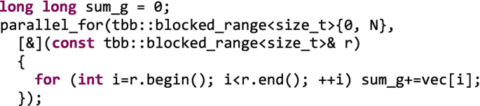
For the sake of backing up all the different alternatives that we have proposed to implement just a simple algorithm like the histogram computation one, let’s recap and elaborate on the pros and cons of each alternative. Figure 5-29 illustrates some of our options with an even simpler vector addition of 800 numbers using eight threads. The corresponding sequential code would be similar to

As in “The Good, the Bad and the Ugly,” the “cast” of this chapter are “The Mistaken, the Hardy, the Laurel, the Nuclear, the Local and the Wise”:

Figure 5-29

Avoid contention when summing 800 numbers with eight threads: (A) atomic: protecting a global sum with atomic operations, (B) local: using enumerable_thread_specific, (C) wise: use parallel_reduce.

• The Mistaken: We can have the eight threads incrementing a global counter, sum_g, in parallel without any further consideration, contemplation, or remorse! Most probably, sum_g will end up being incorrect, and the cache coherence protocol will also ruin performance. You have been warned.

  

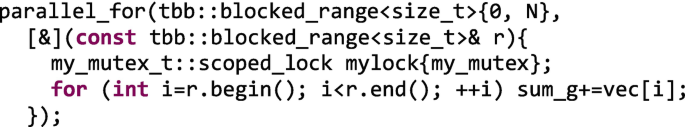
• The Hardy: If we use coarse-grained locking, we get the right result, but usually we also serialize the code unless the mutex implements HTM (as the speculative flavor does). This is the easiest alternative to protect the critical section, but not the most efficient one. For our vector sum example, we will illustrate the coarse-grained locking by protecting each vector chunk accumulation, thus getting a coarse-grained critical section.

  

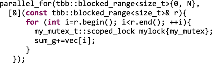
• The Laurel: Fine-grained locking is more laborious to implement and typically requires more memory to store the different mutexes that protect the fine-grained sections of the data structure. The silver lining though is that the concurrency among threads is increased. We may want to assess different mutex flavors to choose the best one in the production code. For the vector sum, we don’t have a data structure that can be partitioned so that each part can be independently protected. Let’s consider a fine-grained implementation the following one in which we have a lighter critical section (in this case is as serial as the coarse-grained one, but threads compete for the lock at finer granularity).

  

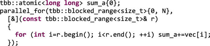
• The Nuclear: In some cases, atomic variables can come to our rescue. For example, when the shared mutable state can be stored in an integral type and the needed operation is simple enough. This is less expensive than the fine-grained locking approach and the concurrency level is on par. The vector sum example (see Figure 5-29(A)) would be as follows, in this case, as sequential as the two previous approaches and with the global variable as highly contended as in the finer-grained case.

  

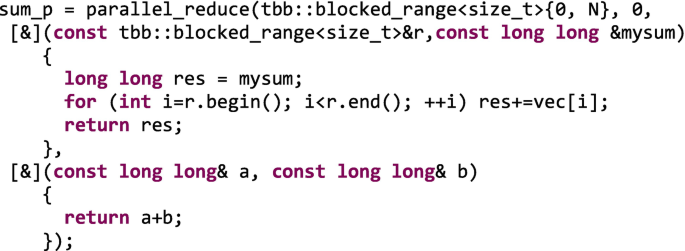
• The Local: Not always can we come up with an implementation in which privatizing local copies of the shared mutable state saves the day. But in such a case, thread local storage, TLS, can be implemented thanks to enumerate_thread_specific, ETS, or combinable classes. They work even when the number of collaborating threads is unknown and convenient reduction methods are provided. These classes offer enough flexibility to be used in different scenarios and can suit our needs when a reduction over a single iteration space does not suffice. To compute the vector sum, we present in the following an alternative in which the private partial sums, priv_s, are later accumulated sequentially, as in Figure 5-29(B).

  

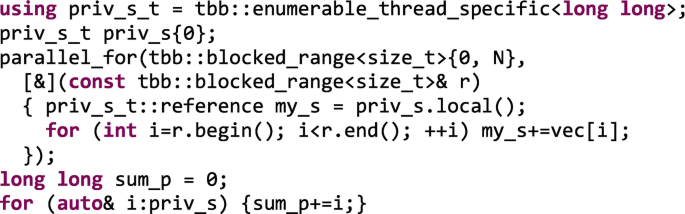
• The Wise: When our computation fits into a reduction pattern, it is highly recommendable to relay on the parallel_reduction template instead of hand-coding the privatization and reduction using the TBB thread local storage features. The following code may look more intricate than the previous one, but wise software architects devised clever tricks to fully optimize this common reduction operation. For instance, in this case the reduction operation follows a tree-like approach with complexity O(log n) instead of O(n), as we see in Figure 5-29(C). Take advantage of what the library puts in your hands instead of reinventing the wheel. This is certainly the method that scales best for a large number of cores and a costly reduction operation.

  

As with the histogram computation, we also evaluate the performance of the different implementations of the vector addition of size 10⁹ on our Core i7 quad-core architecture, as we can see in Figure 5-30. Now the computation is an even finer-grained one (just incrementing a variable), and the relative impact of 10⁹ lock-unlock operations or atomic increments is higher, as can be seen in the speedup (deceleration more properly speaking!) of the atomic (Nuclear) and fine-grained (Laurel) implementations. The coarse-grained (Hardy) implementation takes a slightly larger hit now than in the histogram case. The TLS (Local) approach is only 1.86× faster than the sequential code. Unsafe (Mistaken) is now 3.37× faster than sequential, and now the winner is the parallel_reduction (Wise) implementation that delivers a speedup of 3.53× for four cores.

Figure 5-30

Speedup of the different implementations of the vector addition for N=10⁹ on an Intel Core i7-6700HQ (Skylake)

You might wonder why we went through all these different alternatives to end up recommending the last one. Why did we not just go directly to the parallel_reduce solution if it is the best one? Well, unfortunately, parallel life is hard, and not all parallelization problems can be solved with a simple reduction. In this chapter, we provide you with the devices to leverage synchronization mechanisms if they are really necessary but also show the benefits of rethinking the algorithm and the data structure if at all possible.

Summary

The TBB library provides different flavors of mutexes as well as atomic variables to help us synchronize threads when we need to access shared data safely. The library also provides thread local storage, TLS, classes (as ETS and combinable) and algorithms (as parallel_reduction) that help us avoid the need for synchronization. In this chapter, we walked through the epic journey of parallelizing an image histogram computation. For this running example, we saw different parallel implementations starting from an incorrect one and then iterated through different synchronization alternatives, like coarse-grained locking, fine-grained-locking, and atomics, to end up with some alternative implementations that do not use locks at all. On the way, we stopped at some remarkable spots, presenting the properties that allow us to characterize mutexes, the different kinds of mutex flavors available in the TBB library, and common problems that usually arise when relying on mutexes to implement our algorithms. Now, at the end of the journey, the take-home message from this chapter is obvious: do not use locks unless performance is not your target!

For More Information

Here are some additional reading materials we recommend related to this chapter:

• C++ Concurrency in action, Anthony Williams, Manning Publications, Second Edition, 2018.

• A Primer on Memory Consistency and Cache Coherence, Daniel J. Sorin, Mark D. Hill, and David A. Wood, Morgan & Claypool Publishers, 2011.

Photo of Ronda, Málaga, in Figure 5-1, taken by author Rafael Asenjo, used with permission.

Memes shown within Chapter 5 figures used with permission from 365psd.com “33 Vector meme faces.”

Traffic jam in Figure 5-17 drawn by Denisa-Adreea Constantinescu while a PhD student at the University of Malaga, used with permission.