Electric Circuits

Abstract

In the first part of this book, we examined various mechanical systems. In this chapter, we will study what appears to be a very different type of system—electrical circuits, which have three primary passive elements: resistors, capacitors, and inductors. These elements may seem quite different than the mechanical elements we studied previously: dampers, springs, and masses. However, we will see that there are mathematical analogies between the electrical and mechanical elements that make their behavior nearly identical. Therefore, all of the mathematical tools that we have developed for mechanical systems are directly applicable to the analysis of electrical systems.

Problems

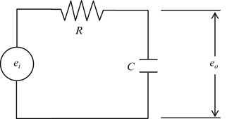
• 1. Consider the R-C circuit shown in the figure. Suppose the input voltage is a step function: e _i (t) = E ₀ ⋅ u(t), where E ₀ = 5 V. The resistance is 100 Ω and the capacitance is 10 μF. Find the time domain differential equation describing the output voltage, e _o (t). Calculate the time constant of the system. Solve the equation for e _o (t) using Laplace transforms assuming the initial charge in the capacitor is zero. Plot e _o (t) using Matlab ^® for four time constants of the system; use units of ms for the time axis. Apply the final value theorem and initial value theorem to the solution in the Laplace domain and show that the results agree with your plot.

  

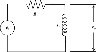
• 2. Consider the R-L circuit shown in the figure. Suppose the input voltage is a step function: e _i (t) = E ₀ ⋅ u(t), where E ₀ = 5 V. The resistance is 100 Ω and the inductance is 10 mH. Find the time domain differential equation describing the output voltage, e _o (t). Calculate the time constant for the system. Solve the equation for e _o (t) using Laplace transforms assuming the initial voltage drop across the inductor is zero. Plot e _o (t) using Matlab ^® for four time constants of the system; use units of ms for the time axis. Apply the final value theorem and initial value theorem to the solution in the Laplace domain and show that the results agree with your plot.

  

• 3. Using the fact that impedance is in units of ohms, prove that the time constants you calculated in Problems 1 and 2 have units of seconds. (Hint: What are the units of the Laplace variable s?)

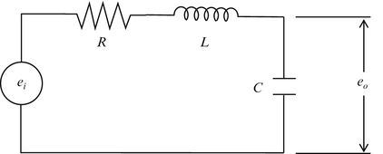
• 4. Consider the R-L-C circuit shown in the figure. Suppose the input voltage is a step function: e _i (t) = E ₀ ⋅ u(t), where E ₀ = 5 V. The initial conditions are zero. The resistance is 50 Ω, the capacitance is 5 μF, and the inductance is 100 mH. Find the time domain differential equation describing the output voltage, e _o (t). Calculate the natural frequency, ω _n , and damping ratio, ζ, for the system. Using a script file in Matlab ^®, find e _o (t) using the ilpalace command and plot e _o (t) for four time constants of the system; use units of ms for the time axis.

  

• 5. Consider the circuit shown in the figure. Using impedance methods, find the transfer function $\frac{E_o(s)}{E_i(s)}$.

  

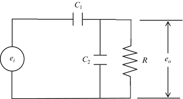
  The values of the system constants are provided.

  $$ \begin{array}{l}{C}_1=0.01\;\mathrm{F}\\ {}{C}_2=0.01\;\mathrm{F}\\ {}\kern0.5em R=100\;\varOmega \end{array} $$

  Using a script file in Matlab ^® and the step command, find and plot the unit step response e _o (t). Apply the final value theorem and initial value theorem to the solution in the Laplace domain and show that the results agree with your plot.

• 6. Consider the circuit shown in the figure. Using impedance methods, find the transfer function $\frac{E_o(s)}{E_i(s)}$.

  

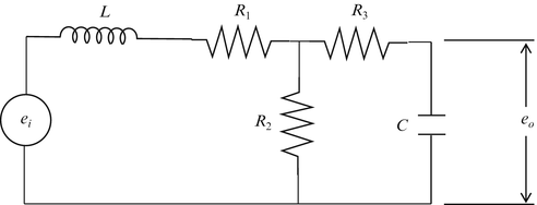
  The values of the system constants are provided.

  $$ \begin{array}{l}\kern0.45em L=0.1\;\mathrm{H}\\ {}\kern0.35em C=1\;\mathrm{F}\\ {}{R}_1=100\;\varOmega \\ {}{R}_2=100\;\varOmega \\ {}{R}_3=150\;\varOmega \end{array} $$

  Using a script file in Matlab ^® and the command step, find and plot the unit step response e _o (t). Apply the final value theorem and initial value theorem to the solution in the Laplace domain and show that the results agree with your plot.

• 7. Consider the circuit shown in the figure. Using impedance methods, find the transfer function $\frac{E_o(s)}{E_i(s)}$.

  

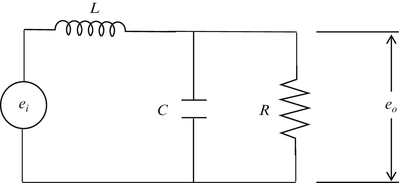
  Choose values for R, L, and C that ensure the system will oscillate. Using a script file in Matlab ^® and the command step, find and plot the unit step response e _o (t) using your values. Apply the final value theorem and initial value theorem to the solution in the Laplace domain and show that the results agree with your plot.

• 8. Consider the op-amp circuit shown in the figure. Using impedance methods, find the transfer function $\frac{E_o(s)}{E_i(s)}$.

  

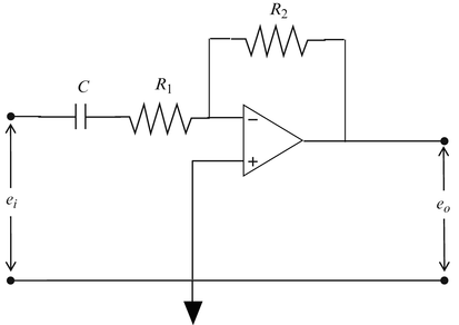
  The values of the system constants are provided.

  $$ \begin{array}{l}\kern0.35em C=20\;\upmu \mathrm{F}\\ {}{R}_1=100\;\varOmega \\ {}{R}_2=200\;\varOmega \end{array} $$

  Using a script file in Matlab ^® and the command step, find and plot the unit step response e _o (t). Apply the final value theorem and initial value theorem to the solution in the Laplace domain and show that the results agree with your plot.

• 9. Consider the op-amp circuit shown in the figure. Using impedance methods, find the transfer function $\frac{E_o(s)}{E_i(s)}$.

  

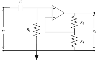
  The values of the system constants are provided.

  $$ \begin{array}{l}\ C=20\kern0.5em \upmu \mathrm{F}\\ {}{R}_1=100\kern0.5em \varOmega \\ {}{R}_2=100\kern0.5em \varOmega \\ {}{R}_3=100\kern0.5em \varOmega \end{array} $$

  Using a script file in Matlab ^® and the command step, find and plot the unit step response e _o (t). Apply the final value theorem and initial value theorem to the solution in the Laplace domain and show that the results agree with your plot.