Frequency Domain Analysis

Abstract

So far, we have mostly examined the response of dynamic systems to relatively simple inputs: impulses, steps, and ramps. While we have used Matlab ^® to calculate the response of systems to more complex inputs numerically, there are also analytical methods that can be used to identify the response of systems to inputs of a general form. The most common analytical method is frequency domain analysis: the analysis of the steady state response for a linear system to sinusoidal (harmonic) inputs.

Problems

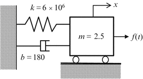
• 1. A single degree of freedom spring-mass-damper system is shown with m = 2.5 kg, k = 6 × 10⁶ N/m, and b = 180 N-s/m. A force harmonic f(t) is applied to the mass.

  

  Complete the following.

  • (a) Calculate the natural frequency ω _n (in rad/s), the damping ratio ζ, the damped natural frequency ω _d (in rad/s), and the resonant frequency ω _r (in rad/s).

  • (b) Find the transfer function $G(s)=\frac{X(s)}{F(s)}$ for the system and then, by replacing s with jω, find the FRF for the system, G( jω).

  • (c) Write a Matlab ^® script file to plot the magnitude (in m/N), phase (in deg), and real and imaginary parts (in m/N) of the FRF.

  • (d) Identify the frequency (in Hz) and amplitude (in m/N) for the key features from the plots.

  • (e) Determine the value of the magnitude of the FRF for this system at a forcing frequency of 1500 rad/s by combining the find and the min or max commands in Matlab ^®. If the harmonic force magnitude is 250 N, determine the amplitude of the steady state response (in mm) at this frequency.

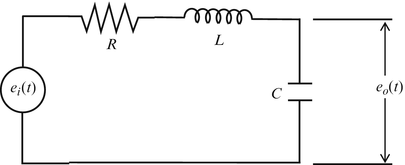
• 2. In the R-L-C circuit shown, the C, L, and R values are 10 μF, 250 mH, and 50 Ω, respectively. The circuit is subjected to a harmonic forcing voltage, e _i (t).

  

  Complete the following.

  • (a) Calculate the natural frequency ω _n (in rad/s), the damping ratio ζ, the damped natural frequency ω _d (in rad/s), and the resonant frequency ω _r (in rad/s).

  • (b) Find the transfer function $G(s)=\frac{E_o(s)}{E_{in}(s)}$ for the system and then, by replacing s with jω, find the FRF of the system, G( jω).

  • (c) Write a Matlab ^® script file to plot the magnitude, phase (in deg), and real and imaginary parts of the FRF.

  • (d) Identify the frequency (in Hz) and amplitude for the key features from the plots.

  • (e) Determine the value of the magnitude of the FRF for this system at a forcing frequency of 600 rad/s by combining the find and the min or max commands in Matlab ^®. If the harmonic voltage magnitude is 5 V, determine the amplitude of the steady state response (in V) at this frequency.

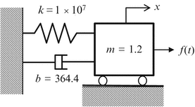
• 3. A single degree of freedom lumped parameter system has mass, stiffness, and damping values of 1.2 kg, 1 × 10⁷ N/m, and 364.4 N-s/m, respectively.

  

  Complete the following.

  • (a) Plot the magnitude (m/N) vs. frequency (Hz) and phase (deg) vs. frequency (Hz) of the FRF.

  • (b) Plot the real part (m/N) vs. frequency (Hz) and imaginary part (m/N) vs. frequency (Hz) of the FRF.

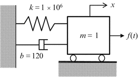
• 4. A single degree of freedom spring-mass-damper system with m = 1 kg, k = 1 × 10⁶ N/m, and b = 120 N-s/m is subjected to forced harmonic vibration.

  

  Complete the following.

  • (a) Calculate the natural frequency ω _n (in rad/s), the damping ratio ζ, the damped natural frequency ω _d (in rad/s), and the resonant frequency ω _r (in rad/s).

  • (b) Write expressions for the real part, imaginary part, magnitude, and phase of the system frequency response function (FRF). These expressions should be written as a function of the frequency ratio, $r=\frac{\omega }{\omega_n}$, stiffness, k, and damping ratio, ζ.

  • (c) Plot the real part (in m/N), imaginary part (in m/N), magnitude (in m/N), and phase (in deg) of the system FRF as a function of the frequency ratio, r. Use a range of 0 to 2 for r (note that r = 1 is near the resonant frequency).

• 5. A single degree of freedom spring-mass-damper system with m = 1.2 kg, k = 1 × 10⁷ N/m, and b = 364.4 N-s/m is subjected to a forcing function f(t) = 15 sin(ω _n t) N, where ω _n is the system’s natural frequency. Determine the steady-state magnitude (in μm) and phase (in deg) of the vibration due to this harmonic force.