Simple Linear Regression and the Correlation Coefficient

Abstract

In Sect. 6.9, we used correlation to provide a measure of the strength of any linear relationship between a pair of random variables X and Y. The random variables are treated perfectly symmetrically; that is, “the correlation between X and Y” is equivalent to “the correlation between Y and X.” In this chapter, we first discuss the linear relationship between a pair of variables without perfect symmetry. In other words, we assume that Y is a dependent variable and X an independent variable: Y depends on X. Then we discuss the bivariate normal relationship and concepts related to the correlation coefficient.

Appendices

Appendix 1: Derivation of Normal Equations and Optimal Portfolio Weights

In this appendix, we derive the normal equations that are used to obtain the least-squares estimates of population regression parameters. For convenience, we denote the function to be minimized as

$$ F=\sum\limits_{i=1}^n {e_i^2=\sum\limits_{i=1}^n {{{{\left( {{y_i}-a-b{x_i}} \right)}}^2}} } $$

(13.36)

Because this function is to be minimized with respect to a and b, it is necessary to take the partial derivatives of F with respect to these two variables. The partial derivatives are

$$ \begin{array}{llll} \frac{{\partial F}}{{\partial a}}=\sum\limits_{i=1}^n {2\left( {{y_i}-a-b{x_i}} \right)\left( {-1} \right)} \hfill \\\frac{{\partial F}}{{\partial b}}=\sum\limits_{i=1}^n {2\left( {{y_i}-a-b{x_i}} \right)\left( {-{x_i}} \right)} \hfill \end{array} $$

Setting these partial derivatives equal to zero yields the following two normal equations:

$$ \begin{array}{llll} \sum\limits_{i=1}^n {{y_i}=na+b\sum\limits_{i=1}^n {{x_i}} } \hfill \cr \sum\limits_{i=1}^n {{x_i}{y_i}=a\sum\limits_{i=1}^n {{x_i}+b\sum\limits_{i=1}^n {x_i^2} } } \hfill \end{array} $$

(13.37)

These are Eqs. 13.12 and 13.13 in the text. Note that setting the first partial equal to zero is identical to requiring that the sum of the residuals be zero because the term in parentheses is the residual e _i  = (y _i – a – bx _i ).

Now we use the technique of deriving Eq. 13.37 to derive the optimal weight of a portfolio. Following Equation (6.29) in Chap. 6, the variance of rates of return for a portfolio is defined as

$$ \begin{array}{llll} \mathrm{ Var}\left( {Rp} \right)&= W_1^2\sigma_1^2+W_2^2\sigma_2^2+2{W_1}{W_2}{\sigma_{12 }} \hfill \cr&\quad \left( {{W_1}+{W_2}=1} \right) \hfill \end{array} $$

(13.38)

where W ₁ and W ₂ represent percentage money invested in security 1 and security 2, respectively; $\sigma_1^2$ = variance of rates of return for security $1,\sigma_2^2$ = variance of rates of return for security 2, and $\sigma_{12 }$ = covariance between the rates of return for security 1 and the rates of return for security 2.

If the objective of the investor is to minimize the variance of a portfolio, then the optimal weights of a two-security portfolio can be obtained by taking partial derivatives of Var(Rp) with respect to the variance of W ₁ and W ₂ = 1 – W ₁ as:

$$ \frac{{\partial \mathrm{ Var}\left( {Rp} \right)}}{{\partial {W_1}}}=2{W_1}\sigma_1^2-2\left( {1-{W_1}} \right)\sigma_2^2+2\left( {1-{W_1}} \right){\sigma_{12 }} $$

Setting this partial derivative to zero and solving for W ₁, we obtain

$$ \begin{array}{llll} {W_1}=\frac{{\sigma_2^2-{\sigma_{12 }}}}{{\sigma_1^2+\sigma_2^2-2{\sigma_{12 }}}}\end{array}$$

(13.39)

$$ {W_2}=1-{W_1}=\frac{{\sigma_1^2-{\sigma_{12 }}}}{{\sigma_1^2+\sigma_2^2-2{\sigma_{12 }}}} $$

(13.40)

Substituting the data of Example 6.21 in Chap. 6 into these two equations, we can estimate W ₁ and W ₂ as¹¹

$$ \begin{array}{llll} {W_1}=\frac{.008+.00375 }{{.00625+.008+2\left( {.00375} \right)}}=.5402 \cr {W_2}=1-.542=.4598 \end{array} $$

Appendix 2: The Derivation of Equation 13.20

The left-hand side of Eq. 13.20 can be written as

$$ \sum\limits_{i=1}^n {{{{\left( {{y_i}-\bar{y}} \right)}}^2}} =\sum\limits_{i=1}^n {{{{\left( {{y_i}-{{\hat{y}}_i}} \right)}}^2}} +2\sum\limits_{i=1}^n {\left( {{y_i}-{{\hat{y}}_i}} \right)} \left( {{{\hat{y}}_i}-\bar{y}} \right)+\sum\limits_{i=1}^n {{{{\left({{{\hat{y}}_i}-\bar{y}} \right)}}^2}} $$

(13.41)

In addition, we know that

$$ \begin{array}{llll} \sum\limits_{i=1}^n {\left( {{y_i}-{{\hat{y}}_i}} \right)} \left( {{{\hat{y}}_i}-\bar{y}} \right) &=\sum\limits_{i=1}^n {\left[ {a+b{x_i}-\left( {a+b\bar{x}} \right)} \right]} \left[ {{y_i}-{{\hat{y}}_i}} \right] \cr& =b\sum\limits_{i=1}^n {\left( {{x_i}-\bar{x}} \right)} \left( {{y_i}-{{\hat{y}}_i}} \right) \\& =-b\bar{x}\sum\limits_{i=1}^n {\left( {{y_i}-\hat{y}} \right)} +b\sum\limits_{i=1}^n {\left( {{y_i}-{{\hat{y}}_i}} \right)} \left( {{x_i}} \right) \end{array} $$

Because assumptions C and A discussed in Sect. 13.4 imply that

$$ \sum\limits_{i=1}^n {\left( {{y_i}-\hat{y}} \right)} =\sum\limits_{i=1}^n {{e_i}=0}\mathrm{ and}\sum\limits_{i=1}^n {\left( {{y_i}-{{\hat{y}}_i}} \right)} \left( {{x_i}} \right)=\sum\limits_{i=1}^n {{e_i}{x_i}=0} $$

Hence,

$$ \sum\limits_{i=1}^n {\left( {{y_i}-{{\hat{y}}_i}} \right)\left( {{{\hat{y}}_i}-\bar{y}} \right)} =0+0=0 $$

(13.42)

Substituting Eq. 13.42 into Eq. 13.41, we obtain Eq. 13.20.

Appendix 3: The Bivariate Normal Density Function

In correlation analysis, we assume a population where both X and Y vary jointly. It is called a joint distribution of two variables. If both X and Y are normally distributed, then we call this known distribution a bivariate normal distribution.

Following Appendix 1 of chap. 7, we can define the probability density function (PDF) of the normally distributed random variables X and Y as

$$ f(X)=\frac{1}{{{\sigma_X}\sqrt{{2\pi }}}}\rm exp\left[ {\frac{{-{{{\left( {X-{\mu_X}} \right)}}^2}}}{{2\sigma_X^2}}} \right], - \infty < X<\infty $$

(13.43)

$$ f(Y)=\frac{1}{{{\sigma_Y}\sqrt{{2\pi }}}}\rm exp\left[ {\frac{{-\left( {Y-{\mu_Y}} \right)}}{{2\sigma_Y^2}}} \right], - \infty < Y<\infty $$

(13.44)

where μ _X and μ _Y are population means for X and Y, respectively; σ _X and σ _Y are population standard deviations of X and Y, respectively; π = 3.1416; and exp represents the exponential function.

If ρ represents the population correlation between X and Y, then the PDF of the bivariate normal distribution can be defined as

$$ \begin{array}{llll} f\left( {X,Y} \right) &=\frac{1}{{2\pi {\sigma_X}{\sigma_Y}\sqrt{{1-{\rho^2}}}}}\exp \left( {-q/2} \right), \hfill \\&\quad- \infty <\; X<\;\infty, -\infty < \;Y\;<\;\infty \hfill \end{array} $$

(13.45)

where σ _X  > 0, σ _Y  > 0, and −1 < ρ < 1,

$$ q=\frac{1}{{1-{\rho^2}}}\left[ {\left( {{{{\left( {\frac{{X-{\mu_X}}}{{{\sigma_X}}}} \right)}}^2}-2\rho \left( {\frac{{X-{\mu_X}}}{{{\sigma_X}}}} \right)\left( {\frac{{Y-{\mu_Y}}}{{{\sigma_Y}}}} \right)+{{{\left( {\frac{{Y-{\mu_Y}}}{{{\sigma_Y}}}} \right)}}^2}} \right)} \right] $$

It can be shown that the conditional mean of Y, given X, is linear in x and given by

$$ E\left( {Y|X} \right)={\mu_Y}+\rho \left\{ {\frac{{{\sigma_Y}}}{{{\sigma_X}}}} \right\}\left( {X-{\mu_X}} \right) $$

(13.46)

It is also clear that given X, we can define the conditional variance of Y as

$$ {\sigma^2}\left( {Y|X} \right)=\sigma_Y^2\left( {1-{\rho^2}} \right) $$

(13.47)

Equation 13.46 can be regarded as describing the population linear regression line. For example, if we have a bivariate normal distribution of heights of brothers and sisters, we can see that they vary together and there is no cause-and-effect relationship. Accordingly, a linear regression in terms of the bivariate normal distribution variable is treated as though there were a two-way relationship instead of an existing causal relationship. It should be noted that regression implies a causal relationship only under a prediction case.

Equation 13.45 represents a joint PDF for X and Y. If p = 0, then Eq. 13.45 becomes

$$ f\left( {X,Y} \right)=f(X)f(Y) $$

(13.48)

This implies that the joint PDF of X and Y is equal to the PDF of X times the PDF of Y. We also know that both X and Y are normally distributed. Therefore, X is independent of Y.

Example 13.5 Using a Mathematics Aptitude Test to Predict Grade in Statistics

Let X and Y represent scores in a mathematics aptitude test and numerical grade in elementary statistics, respectively. In addition, we assume that the parameters in Eq. 13.45 are

$$ \mu_X=550 \,\sigma_X=40\, \mu_Y=80 \sigma_Y=4\rho =.7 $$

Substituting this information into Equations 13.46 and 13.47, respectively, we obtain

$$ \begin{array}{llll} E\left( {Y|X} \right)& =80+.7\left( {4/40} \right)\left( {X-550} \right) \cr &=41.5+.07X \end{array} $$

(13.49)

$$ {\sigma^2}\left( {Y|X} \right)=\left( {16} \right)\left( {1-.49} \right)=8.16 $$

(13.50)

If we know nothing about the aptitude test score of a particular student (say, John), we have to use the distribution of Y to predict his elementary statistics grade.

$$ 95\%\mathrm{ interval} = 80 \pm \left( {1.96} \right)(4)=80\pm 7.84 $$

That is, we predict with 95 % probability that John’s grade will fall between 87.84 and 72.16.

Alternatively, suppose we know that John’s mathematics aptitude score is 650. In this case, we can use Eqs. 13.49 and 13.50 to predict John’s grade in elementary statistics.

$$ E\left( {Y|X=650} \right)=41.5+\left( {.07} \right)\left( {650} \right)=87 $$

and

$$ {\sigma^2}\left( {Y|X=650} \right)=8.16 $$

We can now base our interval on a normal probability distribution with a mean of 87 and a standard deviation of 2.86.

$$ 95 \% \, \mathrm{ interval}=87\pm \left( {1.96} \right)\left( {2.86} \right)=87\pm 5.61 $$

That is, we predict with 95 percent probability that John’s grade will fall between 92.61 and 81.39.

Two things have happened to this interval. First, the center has shifted upward to take into account the fact that John’s mathematics aptitude score is above average. Second, the width of the interval has been narrowed from 87.84−72.16 = 15.68 grade points to 92.61−81.39 = 11.22 grade points. In this sense, the information about John’s mathematics aptitude score has made us less uncertain about his grade in statistics. This issue is discussed in further detail in Sect. 14.4 in the next chapter.

Appendix 4: American Call Option and the Bivariate Normal CDF

The call option pricing model discussed in Appendix 2 of chap. 6 and Appendices 2 and 3 of chap. 7 is derived in terms of an option contract which can be exercised only on the expiration date. This kind of option is called European call. If the contract of a call option can be exercised at any time of the option’s contract period, then this kind of call option is called American call.

When a stock pays a dividend, the American call is more complex. The American call is with one known dividend payment. The valuation equation can be defined as¹²

$$ \begin{array}{llll} C\left( {S,T,X} \right)&= \;{S^x}\left[ {{N_1}\left( {{b_1}} \right)+{N_2}\left( {{a_1},-{b_1};-\sqrt{t/T }} \right)} \right] \cr&\quad - X{e^{-rT }}\left[ {{N_1}\left( {{b_2}} \right){e^{r(T-t) }}+{N_2}\left( {{a_2},-{b_2};-\sqrt{t/T }} \right)} \right] \cr&\quad+ D{e^{-rT }}{N_1}\left( {{b_2}} \right) & \end{array} $$

(13.51)

where

$$ \begin{array}{llll} {a_1}=\frac{{\mathrm{ In}\left( {\frac{{{S^x}}}{X}} \right)+\left( {r+\frac{1}{2}{\sigma^2}} \right)T}}{{\sigma \sqrt{T}}}, &{a_2}={a_1}-\sigma \sqrt{T} \hfill \\& & \hfill \end{array} $$

(13.52)

$$ {b_1}=\frac{{\mathrm{ In}\left( {{{{{S^x}}} \left/ {S} \right.}_t^{*}} \right)+\left( {r+\frac{1}{2}{\sigma^2}} \right)t}}{{\sigma \sqrt{t}}},{b_2}={b_1}-\sigma \sqrt{t} $$

(13.53)

$$ {S^x}=S-D{e^{-rT }} $$

(13.54)

S ^X represents the correct stock net price of the present value of the promised dividend per share (D). t represents the time dividend to be paid.

$$ \begin{array}{llll} S_t^{*} \mathrm{ is} \,\mathrm{ the} \,\mathrm{ ex}\text{--}\mathrm{ dividend}\,\mathrm{ stock}\, \mathrm{ price}\,\mathrm{ for\, the\, American\, call\ option}\, \mathrm{ which} \hfill \\C\left( {S_t^{*},T-t,X} \right)=S_t^{*}+D-X\qquad\qquad\qquad\qquad & \hfill \end{array} $$

(13.55)

S, X, r, σ ², T have been defined in Appendix 3 of chap. 7.

Both N ₁(b ₁) and N ₁(b ₂) are cumulative univariate normal density function. N ₂ (a, b; p) is the cumulative bivariate normal density function with upper integral limits, a and b, and correlation coefficient, $\rho =-\sqrt{t/T }$.

American call option on a non-dividend-paying stock will never optimally be exercised prior to expiration. Therefore, if there exist no dividend payments, Eqs. 13.51, 13.52, 13.53 will reduce to the valuation Equation of the European Option with no dividend payment as defined in Eq. 7.35 of Appendix 2 of chap. 7.

In Appendices 1 and 2 of chap. 7, we have shown how the cumulative univariate normal density function can be used to evaluate the European call option. In this appendix, we found that if a common stock pays a discrete dividend during the option’s life, the American call option valuation equation requires the evaluation of a cumulative bivariate normal density function. While there are many available approximations for the cumulative bivariate normal distribution, the approximation provided here relies on Gaussian quadratures. The approach is straightforward and efficient, and its maximum absolute error is.00000055.

Following Eq. 13.45 in Appendix 3, the probability that x′ is less than a and that y′ is less than b for the standardized cumulative bivariate normal distribution

$$ P\left( {X{\prime}< a,Y{\prime}< b} \right)=\frac{1}{{2\pi \sqrt{{1-{\rho^2}}}}}\int_{{-\infty}}^a {\int_{{-\infty}}^b {\exp \left[ {\frac{{2x{{\prime}^2}-2\rho x{\prime}y{\prime}+y{{\prime}^2}}}{{2\left( {1-{\rho^2}} \right)}}} \right]} dx{\prime}dy{\prime}} $$

where ${x}^{{\prime}}=\frac{{x-{\mu_X}}}{{{\sigma_X}}},{y}^{\prime}\frac{{y-{\mu_Y}}}{{{\sigma_Y}}}$ and ρ is the correlation between the random variables x′ and y′.

The first step in the approximation of the bivariate normal probability N ₂(a,b;ρ) is as follows:

$$ \phi \left( {a,b;\rho } \right)\approx.31830989\sqrt{{1-{\rho^2}}}\sum\limits_{i=1}^5 {\sum\limits_{j=1}^5 {{w_i}{w_j}f\left( {x{^{\prime}_i},x{^{\prime}_j}} \right),} } $$

(13.56)

where

$$ f\left( {x{^{\prime}_i},x{^{\prime}_j}} \right)=\exp \left[ {{a_1}\left( {2x{^{\prime}_i}-{a_1}} \right)+{b_1}\left( {2x{^{\prime}_j}-{b_1}} \right)+2\rho \left( {x{^{\prime}_i}-{a_1}} \right)\left( {x{^{\prime}_j}-{b_1}} \right)} \right], $$

The pairs of weights (w) and corresponding abscissa values (x′) are¹³

i, j	w	x′
1	.24840615	.10024215
2	.39233107	.48281397
3	.21141819	1.0609498
4	.033246660	1.7797294
5	.00082485334	2.6697604

and the coefficients a ₁ and b ₁ are computed using

$$ {a_1}=\frac{a}{{\sqrt{{2\left( {1-{\rho^2}} \right)}}}}\mathrm{ and}\,{b_1}=\frac{b}{{\sqrt{{2\left( {1-{\rho^2}} \right)}}}} $$

The second step in the approximation involves computing the product abρ.

If abρ ≤ 0, compute the bivariate normal probability, N ₂ (a,b;ρ), using the following rules:

$$ \begin{array}{llll} 1.\mathrm{ If}a\le0,b\le 0,\mathrm{ and}\rho \le 0,\mathrm{ then}{N_2}\left( {a,b;\rho } \right)=\phi \left( {a,b;\rho } \right). \hfill \\2.\mathrm{ If}a\le0,b\ge 0,\mathrm{ and}\rho >0,\mathrm{ then}\ {N_2}\left( {a,b;\rho } \right)={N_1}(a)-\phi \left( {a,-b;-\rho } \right). \hfill \\3.\mathrm{ If}a\ge0,b\le 0,\mathrm{ and}\rho >0,\mathrm{ then}{N_2}\left( {a,b;\rho } \right)={N_1}(b)-\phi \left( {-a,b;-\rho } \right). \hfill \\4.\mathrm{ If}a\ge0,b\ge 0,\mathrm{ and}\rho \le 0,\mathrm{ then}{N_2}\left( {a,b;\rho } \right)={N_1}(a)+{N_1}(b)-1+\phi \left( {-a,-b;\rho } \right). \hfill \end{array} $$

(13.57)

If abρ > 0, compute the bivariate normal probability, N ₂ (a,b; ρ), as

$$ {N_2}\left( {a,b;\rho } \right)={N_2}\left( {a,0;{\rho_{ab }}} \right)+{N_2}\left( {b,0;{\rho_{ba }}} \right)-\delta $$

(13.58)

where the values of N ₂ (•) on the right-hand side are computed from the rules for abρ ≤ 0,

$$ \begin{array}{llll} {\rho_{ab }}=\frac{{\left( {\rho a-b} \right)\mathrm{ Sgn}(a)}}{{\sqrt{{{a^2}-2\rho ab+{b^2}}}}}, \;\quad\quad& {\rho_{ba }}=\frac{{\left( {\rho b-a} \right)\mathrm{ Sgn}(b)}}{{\sqrt{{{a^2}-2\rho ab+{b^2}}}}} \\\delta =\frac{{1-\mathrm{ Sgn}(a)\times \mathrm{ Sgn}(b)}}{4} \end{array} $$

and

$$ \mathrm{ S}gn(x)=\left\{ \begin{array}{llll} 1x\ge 0 \hfill \\-1\quad x<0 \hfill \end{array} \right. $$

N ₁(d) is the cumulative univariate normal probability.

Example 13.6 Valuating American Option

An American call option whose exercise price is $45 has an expiration time of 90 days. Assume the risk-free rate of interest is 8 percent annually, the underlying price is $50, the standard deviation of the rate of return of the stock is 20 percent, and the stock pays a dividend of $1.5 in exactly 50 days, (a) what is the European call value? (b) Can the early exercise be predicted? (c) What is the value of the American call?

• (a) The current stock net price of the present value of the promised dividend is

  $$ {s^x} = 50 - \left( {1.5} \right){e^{{-0.8\left( {\frac{50 }{365 }} \right)}}} = 48.516 $$

  Following Equation 7B.2, the European call value can be calculated as

  $$ C = \left( {48.516} \right)N\left( {{d_1}} \right) - \left( {45} \right)\left( {{e^{{-0.8\left( {\frac{90 }{365 }} \right)}}}} \right)N\left( {{d_2}} \right) $$

  where

  $$ \begin{array}{llll} {d_1}& = \frac{{[\mathrm{ In}(48.516/45) + (.08 +.5{(.20)^2})(90/365)]}}{{.20\sqrt{90/365 }}} \cr &= \frac{{.075 +.025}}{.099 } \cr& = 1.010 \cr {d_2}& = 1.010 -.099 =.911 \end{array} $$

  From Table A.l, we obtain

  $$ \begin{array}{llll} N\left( {1.010} \right) =.5 +.3438 =.8438 \\N\left( {.911} \right) =.5 +.3186 =.8186 \end{array} $$

  So the European call value is

  $$ \begin{array}{llll} C& = \left( {48.516} \right)\left( {.8438} \right) - 45\left( {.980} \right)\left( {.8186} \right) \cr& = 4.8375 \end{array} $$

• (b) The present value of the interest income that would be earned by deferring exercise until expiration is

  $$ \begin{array}{llll} X(1 - {e^{-r(T-t) }})& = (45)[1 - {e^{{-.08(90\text{--} 50)/365}}}] \cr& = 45[1 -.991] \cr& =.405 \end{array} $$

  Since d = 1.5 > .405, therefore, the early exercise is not precluded.

• (c) The value of the American call is now calculated as

  $$ \begin{array}{llll} C& = \; \left( {48.208} \right)\left[ {{N_1}\left( {{b_1}} \right) + {N_2}\left( {{a_1}, - {b_1}; - \sqrt{50/90 }} \right)} \right] \cr &\quad- \left( {45} \right){e^{{-.08\left( {90/365} \right)}}}\left[ {{N_1}\left( {{b_2}} \right){e^{{.08\left( {40/365} \right)}}} + {N_2}\left( {{a_2}, - {b_2}; - \sqrt{50/90 }} \right.} \right] \cr&\quad + 2{e^{{-.08\left( {50/365} \right)}}}{N_1}\left( {{b_2}} \right) &&\end{array} $$

  (13.59)

  since both b ₁ and b ₂ depend on the critical ex-dividend stock price $S_t^{*}$, which can be determined by

  $$ C\left( {S_t^{*},40/365;45} \right) = S_t^{*} + 1.5 - 45 $$

  By using trial and error, we find that $S_t^{*} = 44.756$. An Excel program used to calculate this value is presented in Fig. 13.11.

  Fig. 13.11

  

  Microsoft Excel program for calculating $S_t^{*}$

  Substituting S ^x = 48.208, X = $45, and $S_t^{*}$ into Eqs. 13.52 and 13.53, we can calculate a ₁, a ₂, b ₁, and b ₂ as follows:

  $$ \begin{array}{llll} {a_1} = {d_1} = 1.010 \cr {a_2} = {d_2} =.911 \cr {b_1} = \frac{{\mathrm{ In}\displaystyle\left( {\frac{48.516}{44.756}} \right)+\left[ {.08 + \frac{1}{2}{{{\left( {.20} \right)}}^2}} \right]\displaystyle\left( {\frac{50 }{365 }} \right)}}{{\left( {.20} \right)\sqrt{50/365 }}} \cr\quad = \frac{{.0807 +.0137}}{.0740}1.2757 \cr {b_2} = 1.2757 -.0740 = 1.2017 \end{array} $$

  In addition, we also know $\rho =\sqrt{{\tfrac{50 }{90 }}}=.7454$.

  From the above information, we now calculate the related normal probability as follows:

  Using Equation 7A.9 in Appendix 7A, we obtain

  $$ \begin{array}{llll} {N_1}\left( {{b_1}} \right) = {N_1}\left( {1.2757} \right) =.8988 \\{N_1}\left( {{b_2}} \right) = N\left( {1.2017} \right) =.8851 \end{array} $$

  Following Eq. 13.58, we now calculate the values of N ₂(1.010, −1.2757; −.7454) and 7 N ₂(.911, −1.2017; −.7454) as follows:

  Since abρ > 0 for both cumulative bivariate normal density function, therefore, we can use Eq. 13.58 to calculate the value of both N ₂(a,b,ρ) as follows:

  $$ \begin{array}{llll} {\rho_{ab }} = \frac{{\left[ {\left( {-.7454} \right)\left( {1.010} \right) + 1.2757} \right](1)}}{{\sqrt{{{{{\left( {1.010} \right)}}^2} - 2\left( {-.7454} \right)\left( {1.010} \right)\left( {-1.2757} \right)+{{{\left( {-1.2757} \right)}}^2}}}}} =.6133 \hfill \cr {\rho_{ba }} = \frac{{\left[ {\left( {-.7454} \right)\left( {-1.2757} \right) - 1.010} \right]\left( {-1} \right)}}{{\sqrt{{{{{\left( {1.010} \right)}}^2} - 2\left( {-.7454} \right)\left( {1.010} \right)\left( {-1.2757} \right) + {{{\left( {-1.2757} \right)}}^2}}}}} =.0693 \hfill \cr \delta = \frac{{1 - (1)\left( {-1} \right)}}{4} = \frac{1}{2}. \hfill \cr {N_2}\left( {1.010, - 1.2757; -.7454} \right) = {N_2}\left( {1.010,0,.6133} \right) + {N_2}\left( {-1.2757,0;0693} \right) -.5 \hfill \cr = {N_1}(0) + {N_1}\left( {-1.2757} \right) - \phi\left( {-1.010,0; -.6133} \right) - \phi\left( {-1.2757,0; -.0693} \right) -.5 \hfill \cr =.5 +.1010 -.0202 -.0456 -.5 =.0352 \hfill \end{array} $$

  Using Microsoft Excel programs presented in Figs. 13.12 and 13.13, we obtain

  $$ \begin{array}{llll} \phi \left( {-1.010,0;.6133} \right) =.0202 \hfill \cr \phi \left( {-1257,0; -.0693} \right) =.0460 \hfill \\ {N_2}\left( {1.010, - 1.2757; -.7454} \right) = 0.0350 \hfill \cr \phi \left( {-.911,0; -.6559} \right) =.0218 \hfill \cr \phi \left( {-1.2017,0; -.0143} \right) =.0563 \hfill \cr {N_2}\left( {.911, - 1.2017; -.7454} \right) = 0.0368 \hfill \end{array} $$

  Substituting the related information into Eq. 13.59, we obtain

  $$ \begin{array}{llll} C = \left( {48.208} \right)\left[ {.8988 +.0350} \right] \cr \quad\; - \left( {45} \right){e^{{-.08\left( {90/365} \right)}}}\left[ {\left( {.8851} \right){e^{{-.08\left( {40/365} \right)}}} +.0368} \right] \cr \quad\; + 2{e^{{-.08\left( {50/365} \right)}}}\left( {.8851} \right) \cr = \rm\$5.603 \end{array} $$

  All related results are presented in column C of Fig. 13.13.¹⁴

  Fig. 13.12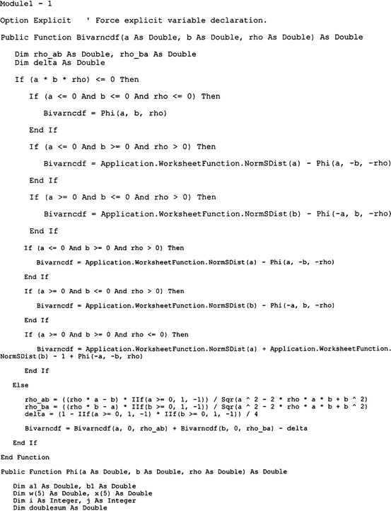

  

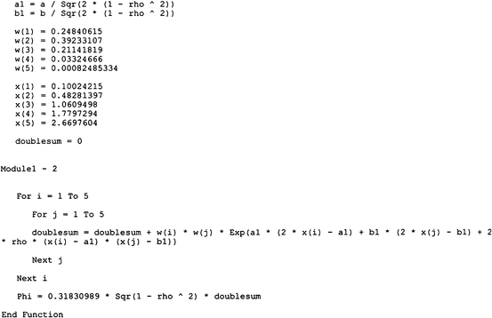
  Microsoft Excel program for calculating function Phi (φ)

  Fig. 13.13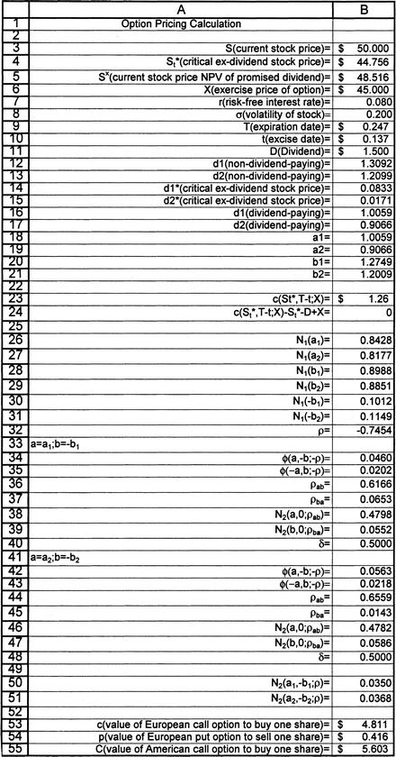

  

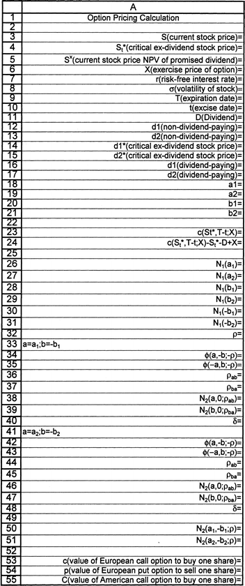
  Microsoft Excel program for calculating two alternative American call options