Model Development by Modal Analysis

Abstract

In Chaps. 1–5, we assumed a model and then used that model to determine the system response in the time or frequency domain (or both). More often, however, we have an actual dynamic system and would like to build a model that we can use to represent its vibratory behavior in response to some external excitation. For example, in milling operations, the flexibility of the cutting tool–holder–spindle–machine structure (and sometimes the workpiece) determines the limiting axial depth of cut to avoid chatter, a self-excited vibration (Schmitz and Smith 2009). In this case, the dynamic response at the free end of the tool (and/or at the cutting location on the workpiece) is measured. Using this measured response, a model in the form of modal parameters can be developed for use in a time-domain simulation¹ of the milling process. How can we work this “backward problem” of starting with a measurement and developing a model? To begin, we need to determine the modal mass, stiffness, and damping values from the measured frequency response function (FRF).

Exercises

• 1. For a single-degree-of-freedom spring–mass–damper system subject to forced harmonic vibration, the measured FRF is displayed in Figs. P6.1a and P6.1b. Using the peak picking method, determine m (in kg), k (in N/m), and c (in N-s/m).

  Fig. P6.1a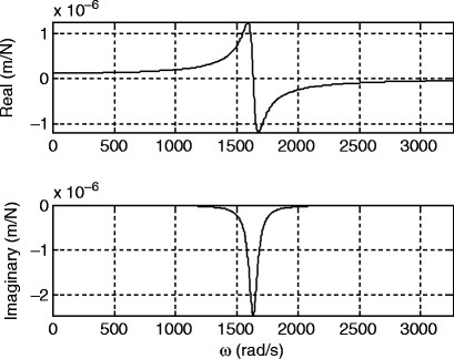

  

  Measured FRF

  Fig. P6.1b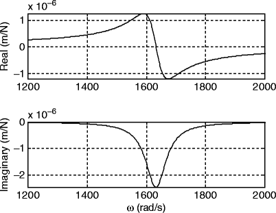

  

  Measured FRF (smaller frequency scale)

• 2. The direct and cross FRFs for the two degree of freedom system shown in Fig. P6.2a are provided in Figs. P6.2b and P6.2c.

  Fig. P6.2a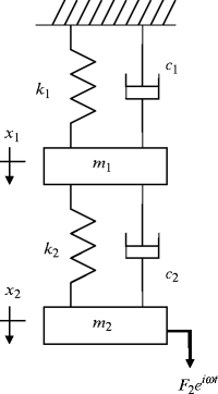

  

  Two degree of freedom spring-mass-damper system under forced vibration

  Fig. P6.2b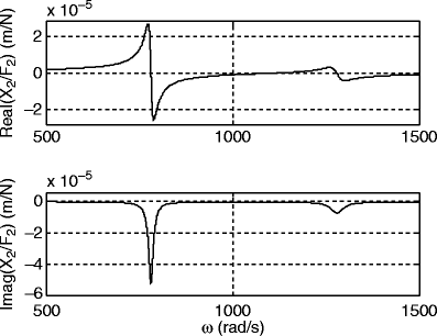

  

  Direct FRF X ₂/F ₂

  Fig. P6.2c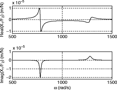

  

  Cross FRF X ₁/F ₂

  • (a) If the modal damping ratios are ζ _q1 = 0.01 and ζ _q2 = 0.016, determine the modal stiffness values k _q1 and k _q2 (N/m) by peak picking.

  • (b) Determine the mode shapes by peak picking.

• 3. An FRF measurement was completed to give the two degree of freedom response shown in Fig. P6.3. Use the peak picking approach to identify the modal mass, stiffness, and damping parameters for the two modes. Arrange your results in the 2 × 2 modal matrices m _q , c _q , and k _q .

  Fig. P6.3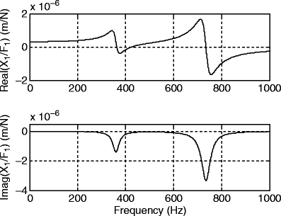

  

  Measured direct FRF for two degree of freedom system

• 4. An FRF measurement was completed to give the two degree of freedom response shown in Fig. P6.4 (a limited frequency range is displayed to aid in the peak picking activity).

  Fig. P6.4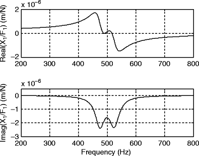

  

  FRF measurement for two degree of freedom system

  • (a) Use the peak picking approach to identify the modal mass, stiffness, and damping parameters for the two modes. Arrange your results in the 2×2 modal matrices m _q , c _q , and k _q .

  • (b) The FRF “measurement” in part (a) was defined using the following Matlab ^® code.

    

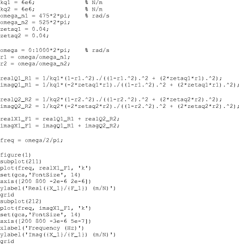
  Plot your modal fit together with the measured FRF and comment on their agreement.

• 5. Figures P6.5a through P6.5e show direct, X ₁/F ₁, and cross FRFs, X ₂/F ₁ through X ₅/F ₁, measured on a fixed-free beam. They were measured at the beam’s free end and in 20 mm increments toward its base; see Fig. 6.36. Determine the mode shape associated with the 200 Hz natural frequency.

  Fig. P6.5a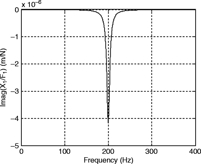

  

  Direct FRF X ₁/F ₁

  Fig. P6.5b

  

  Cross FRF X ₂/F ₁

  Fig. P6.5c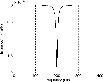

  

  Cross FRF X ₃/F ₁

  Fig. P6.5d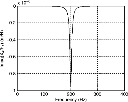

  

  Cross FRF X ₄/F ₁

  Fig. P6.5e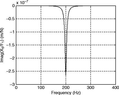

  

  Cross FRF X ₅/F ₁

  Fig. P6.5f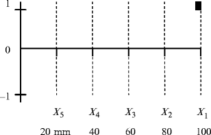

  

  Coordinates for direct and cross FRF measurements

  When plotting the mode shape, normalize the free end response at coordinate x ₁ to 1 (this is normalizing the mode shape to x ₁) and show the relative amplitudes at the other coordinates x ₂ through x ₅. See Fig. P6.5f.

• 6. For the same fixed-free beam as Problem 5, the measurement bandwidth was increased so that the first three modes were captured. Again, the direct, X ₁/F ₁, and cross FRFs, X ₂/F ₁ through X ₅/F ₁, were measured. The imaginary part of the direct FRF for the entire bandwidth is shown in Fig. P6.6a. The three natural frequencies are 200, 550, and 1,250 Hz.

  Fig. P6.6a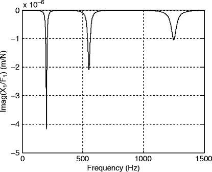

  

  Direct FRF X ₁/F ₁

  Use Figs. P6.6b through P6.6f to identify the mode shape that corresponds to the 1,250 Hz natural frequency. Plot your results using the same approach described in Problem 5.

  Fig. P6.6b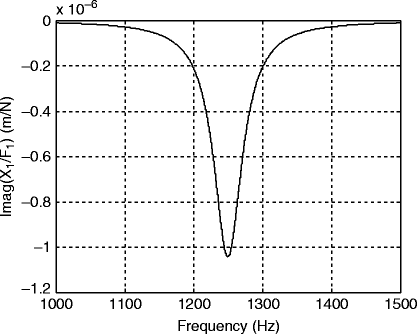

  

  Direct FRF X ₁/F ₁ (mode 3 only)

  Fig. P6.6c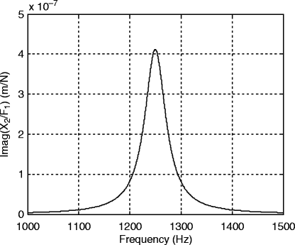

  

  Cross FRF X ₂/F ₁

  Fig. P6.6d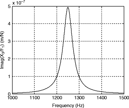

  

  Cross FRF X ₃/F ₁

  Fig. P6.6e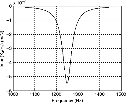

  

  Cross FRF X ₄/F ₁

  Fig. P6.6f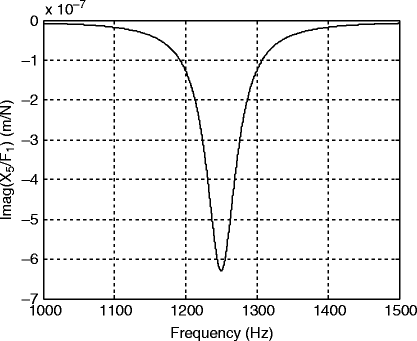

  

  Cross FRF X ₅/F ₁

• 7. Find the mass matrix (in local coordinates) for the two degree of freedom system displayed in Fig. P6.7 using the shortcut method described in Sect. 6.6 if m ₁ = 10 kg and m ₂ = 12 kg.

  Fig. P6.7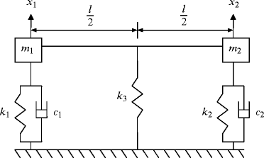

  

  Two degree of freedom system with a rigid, massless bar connecting the two masses, m ₁ and m ₂

• 8. Find the stiffness matrix (in local coordinates) for the two degree of freedom system displayed in Fig. P6.7 using the shortcut method described in Sect. 6.6 if k ₁ = 2 × 10⁵ N/m, k ₂ = 2 × 10⁵ N/m, and k ₃ = 1 × 10⁵ N/m.

• 9. Find the mass matrix (in local coordinates) for the two degree of freedom system displayed in Fig. P6.9 using the shortcut method described in Sect. 6.6 if m ₁ = 10 kg and m ₂ = 12 kg.

  Fig. P6.9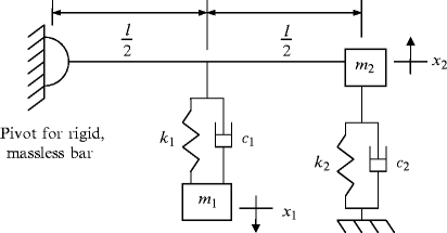

  

  Two degree of freedom system with a rigid, massless bar connecting the mass, m ₂, to a fixed pivot

• 10. Find the stiffness matrix (in local coordinates) for the two degree of freedom system displayed in Fig. P6.9 using the shortcut method described in Sect. 6.6 if k ₁ = 2 × 10⁵ N/m, k ₂ = 2 × 10⁵ N/m, and k ₃ = 1 × 10⁵ N/m.

References

Blevins RD (2001) Formulas for natural frequency and mode shape. Krieger, Malabar (Table 8–1)
Schmitz T, Smith KS (2009) Machining dynamics: Frequency response to improved productivity. Springer, New York
Author information
Authors and Affiliations
Corresponding author