Single Degree of Freedom Forced Vibration

Abstract

Let’s continue our study of the lumped parameter spring–mass–damper model, but now consider forced vibration. While the oscillation decays over time for a damped system under free vibration, the vibratory motion is maintained at a constant magnitude and frequency when an external energy source (i.e., a forcing function) is present.

Exercises

• 1. An apparatus known as a centrifuge is commonly used to separate solutions of different chemical compositions. It operates by rotating at high speeds to separate substances of different densities.

  Fig. P3.1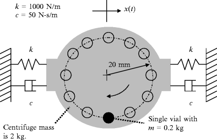

  

  Centrifuge model with a single vial

  • (a) If a single vial with a mass of 0.2 kg is placed in the centrifuge (see Fig. P3.1) at a distance of 20 mm from the rotating axis, determine the magnitude of the resulting vibration, X (in mm), of the single degree of freedom centrifuge structure. The rotating speed is 200 rpm.

  • (b) Determine the magnitude of the forcing function (in N) due to the single 0.2 kg vial rotating at 200 rpm.

• 2. For a single degree of freedom spring–mass–damper system with m = 2.5 kg, k = 6 × 10⁶ N/m, and c = 180 N-s/m, complete the following for the case of forced harmonic vibration.

  • (a) Calculate the undamped natural frequency (in rad/s) and damping ratio.

  • (b) Sketch the imaginary part of the system FRF versus frequency. Identify the frequency (in Hz) and amplitude (in m/N) of the key features.

  • (c) Determine the value of the imaginary part of the vibration (in mm) for this system at a forcing frequency of 1500 rad/s if the harmonic force magnitude is 250 N.

• 3. A single degree of freedom lumped parameter system has mass, stiffness, and damping values of 1.2 kg, 1 × 10⁷ N/m, and 364.4 N-s/m, respectively. Generate the following plots of the frequency response function.

  • (a) Magnitude (m/N) versus frequency (Hz) and phase (deg) versus frequency (Hz)

  • (b) Real part (m/N) versus frequency (Hz) and imaginary part (m/N) versus frequency (Hz)

  • (c) Argand diagram, real part (m/N) versus imaginary part (m/N).

• 4. For the single degree of freedom torsional system under harmonic forced vibration (see Fig. P3.4), complete parts a through c if J = 40 kg-m²/rad, C = 150 N-m-s/rad, K = 5 × 10⁵ N-m/rad, and T ₀ = 65 N-m.

  Fig. P3.4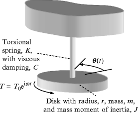

  

  Single degree of freedom torsional system under harmonic forced vibration

  • (a) Calculate the undamped natural frequency (rad/s) and damping ratio.

  • (b) Sketch the Argand diagram (complex plane representation) of $\frac{\theta }{T}\left( \omega \right)$. Numerically identify key frequencies (rad/s) and amplitudes (rad/N-m).

  • (c) Given a forcing frequency of 100 rad/s for the harmonic external torque, determine the phase (in rad) between the torque and corresponding steady-state vibration of the system, θ.

• 5. For a single degree of freedom spring–mass–damper system subject to forced harmonic vibration with m = 1 kg, k = 1 × 10⁶ N/m, and c = 120 N-s/m, complete the following.

  • (a) Calculate the damping ratio.

  • (b) Write expressions for the real part, imaginary part, magnitude, and phase of the system frequency response function (FRF). These expressions should be written as a function of the frequency ratio, r, stiffness, k, and damping ratio, ζ.

  • (c) Plot the real part (in m/N), imaginary part (in m/N), magnitude (in m/N), and phase (in deg) of the system frequency response function (FRF) as a function of the frequency ratio, r. Use a range of 0 to 2 for r (note that r = 1 is the resonant frequency). [Hint: for the phase plot, try using the Matlab ^® atan2 function. It considers the quadrant dependence of the tan⁻¹ function.]

• 6. A single degree of freedom spring–mass–damper system which is initially at rest at its equilibrium position is excited by an impulsive force over a time interval of 1.5 ms; see Fig. P3.6. If the mass is 2 kg, the stiffness is 1 × 10⁶ N/m, and the viscous damping coefficient is 10 N-s/m, complete the following.

  Fig. P3.6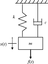

  

  Spring–mass–damper system excited by an impulsive force

  • (a) Determine the maximum allowable force magnitude if the maximum deflection is to be 1 mm.

  • (b) Plot the impulse response function, $h(t)$, for this system. Use a time step size of 0.001 s.

  • (c) Calculate the impulse of the force (N-s).

• 7. For a single degree of freedom spring–mass–damper system subject to forced harmonic vibration, the following FRF was measured (two figures are provided with different frequency ranges). Using the “peak picking” fitting method, determine m (in kg), k (in N/m), and c (in N-s/m).

  Fig. P3.7a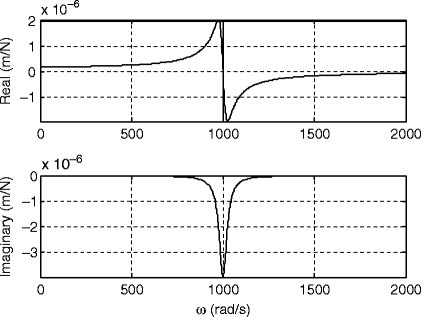

  

  Measured FRF

  Fig. P3.7b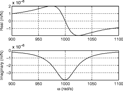

  

  Measured FRF (smaller frequency scale)

• 8. For a single degree of freedom spring–mass–damper system with m = 2 kg, k = 1 × 10⁷ N/m, and c = 200 N-s/m, complete the following for the case of forced harmonic vibration.

  • (a) Calculate the natural frequency (in rad/s) and damping ratio.

  • (b) Plot the Argand diagram (real part vs imaginary part of the system FRF).

  • (c) Identify the point on the Argand diagram that corresponds to resonance.

  • (d) Determine the magnitude of vibration (in m) for this system at a forcing frequency of 2,000 rad/s if the harmonic force magnitude is 100 N.

• 9. In a crank-slider setup, it is desired to maintain a constant rotational speed for driving the crank. Therefore, a flywheel was added to increase the spindle inertia and reduce the speed sensitivity to the driven load. See Fig. P3.9. If the spindle rotating speed is 120 rpm, determine the maximum allowable eccentricity-mass product, me (in kg-m), for the flywheel if the spindle vibration magnitude is to be less than 25 μm. The total spindle/flywheel mass is 10 kg, the effective spring stiffness (for the spindle and its support) is 1 × 10⁶ N/m, and the corresponding damping ratio is 0.05 (5%).

  Fig. P3.9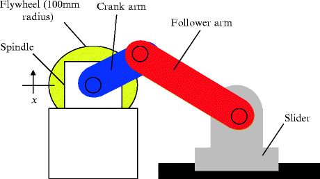

  

  Crank-slider with flywheel

  Given your me result, comment on the accuracy requirements for the flywheel manufacture (you may assume no rotating unbalance in the spindle).

• 10. A single degree of freedom spring–mass–damper system with m = 1.2 kg, k = 1 × 10⁷ N/m, and c = 364.4 N-s/m is subjected to a forcing function $f(t) = 15{e^{{i{\omega_n}t}}}\;{\hbox{N}}$, where ${\omega_n}$ is the system’s natural frequency. Determine the steady-state magnitude (in μm) and phase (in deg) of the vibration due to this harmonic force.

References

Kamen E (1990) Introduction to signals and systems, 2nd edn. Macmillan, New York
Smith S (2000) Flexures: elements of elastic mechanisms. CRC Press, Boca Raton
Xu Z, Naughton J, Lindberg W (2009) 2-D and 3-D numerical modelling of a dynamic resonant shear stress sensor. Comput Fluids 38:340–346
Author information
Authors and Affiliations
Corresponding author