Single Degree of Freedom Free Vibration

Abstract

For the discussions in this chapter, we will use what is referred to as a lumped parameter model to describe free vibration. The “lumped” designation means that the mass is concentrated at a single coordinate (degree of freedom) and it is supported by a massless spring and damper. Recall from Sect. 1.2.1 that free vibration means that the mass is disturbed from its equilibrium position and vibration occurs at the natural frequency, but a long-term external force is not present.

Exercises

• 1. For a single degree of freedom spring–mass system with m = 1 kg and k = 4 × 10⁴ N/m, complete the following for the case of free vibration.

  • (a) Determine the natural frequency in Hz and the corresponding period of vibration.

  • (b) Given an initial displacement of 5 mm and zero initial velocity, write an expression for the time response of free vibration using the following form:

    $$ x(t) = {X_1}{e^{{i{\omega_n}t}}} + {X_2}{e^{{ - i{\omega_n}t}}}\;{\hbox{mm}} $$

  • (c) Plot the first ten cycles of motion for the result from part (b).

• 2. For a single degree of freedom spring–mass system, complete the following.

  • (a) If the free vibration is described as $x(t) = A\cos \left( {{\omega_n}t + {\Phi_c}} \right)$, determine expressions for A and Φ _c if the initial displacement is x ₀ and the initial velocity is ${\dot{x}_0}$.

  • (b) If the free vibration is described as $x(t) = A\cos \left( {{\omega_n}t} \right) + B\sin \left( {{\omega_n}t} \right)$, determine expressions for A and B if the initial displacement is x ₀ and the initial velocity is ${\dot{x}_0}$.

• 3. The differential equation of motion for a cylinder rolling on a concave cylindrical surface is $\ddot{\theta } + \frac{2}{3}\frac{g}{{R - r}}\theta = 0$, where g is the gravitational constant.

  Fig. P2.3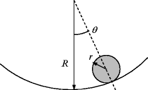

  

  Cylinder rolling on a concave cylindrical surface

  • (a) Write the expression for the natural frequency, ω _n (rad/s).

  • (b) If the free vibration is described as $\theta (t) = A\sin \left( {{\omega_n}t + {\Phi_s}} \right)$, determine expressions for A and Φ _s if the initial angle is θ ₀ and the initial angular velocity is ${\dot{\theta }_0}$.

  • (c) If R = 200 mm, r = 10 mm, θ ₀ = 5° = 0.087 rad, and ${\dot{\theta }_0} = 0$, plot $\theta (t)$ (deg) using the function from part b for the time interval from t = 0 to 5 s in steps of 0.005 s.

• 4. For a single degree of freedom spring–mass–damper system with m = 1 kg, k = 4×10⁴ N/m, and c = 10 N-s/m, complete the following for the case of free vibration.

  • (a) Calculate the natural frequency (in rad/s), damping ratio, and damped natural frequency (in rad/s).

  • (b) Given an initial displacement of 5 mm and zero initial velocity, write the expression for the underdamped, free vibration in the form $x(t) = {e^{{ - \zeta {\omega_n}t}}}\left( {A\cos \left( {{\omega_d}t} \right) + B\sin \left( {{\omega_d}t} \right)} \right)$ mm.

  • (c) Plot the first ten cycles of motion.

  • (d) Calculate the viscous damping value, c (in N-s/m), to give the critically damped case for this system.

• 5. For a single degree of freedom spring–mass–damper system with m = 0.2 lb_m, k = 2.5×10³ lb_f/in., c = 10.92 lb_f-s/ft, x ₀ = 0.1 in., and ${\dot{x}_0} = 0$, complete the following for the case of free vibration.

  Fig. P2.5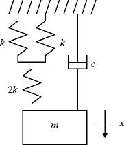

  

  Single degree of freedom spring–mass–damper system under free vibration

  • (a) Determine the equivalent spring constant (in lb_f/in) for the spring configuration shown in the figure.

  • (b) Determine the force (in lb_f) required to cause the initial displacement of 0.1 in. (assume the system was at static equilibrium prior to introducing the initial displacement).

  • (c) Calculate the damping ratio. You will need the units correction factor: (32.2 ft-lb_m)/(lb_f-s²). Is this system underdamped or overdamped?

  • (d) Calculate the damped natural frequency (in Hz).

• 6. For a single degree of freedom spring–mass–damper system under free vibration, determine the values for the mass, m (kg), viscous damping coefficient, c (N-s/m), and spring constant, k (N/m), given the following information:

  • the damping ratio is 0.1

  • the undamped natural frequency is 100 Hz

  • the initial displacement is 1 mm

  • the initial velocity is 5 mm/s

  • if the system was critically damped, the value of the damping coefficient would be 586.1 N-s/m.

• 7. For a single degree of freedom spring–mass–damper system under free vibration, the following information is known: m = 2 kg, k = 1×10⁶ N/m, c = 500 N-s/m, x ₀ = 4 mm, and ${\dot{x}_0} = 0$ mm/s.

  Determine the corresponding expression for velocity (mm/s) if position is given in the form $x(t) = A{e^{{ - \zeta {\omega_n}t}}}\cos \left( {{\omega_d}t + {\varphi_c}} \right)$. Numerically evaluate all coefficients and constant terms in your final expression.

• 8. The requirement for small features on small parts has led to increased demands on measuring systems. One approach for determining the size of features (such as a hole’s diameter) is to use a probe to touch the surface at several locations (e.g., points on the hole wall) and then use these coordinates to calculate the required dimension. To probe small features, small probes are required. However, at small size and force scales, intermolecular forces can dominate.

  An example is the interaction between very small, flexible probes and surfaces. As shown in Fig. P2.8, a 72-μm diameter probe tip comes into contact with a measurement surface (1) and the probe begins to deflect. The attractive (van der Waals) force between the probe and surface causes the tip to “stick” to the surface as it is retracted after contact (2). The motion is provided by an axis which moves the probe relative to the surface. Once the retraction force on the probe overcomes the attractive force, the probe is released from the surface (3) and it oscillates under free vibration conditions. Given the probe’s free vibration response, determine the damping ratio using the logarithmic decrement approach. The peaks from the free vibration response are provided in Table P2.8. (The data in Fig. P2.8 is courtesy of IBS Precision Engineering, Eindhoven, The Netherlands.)

  Fig. P2.8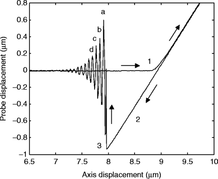

  

  Probe displacement as a function of the axis position

  Table P2.8 Peak values for probe-free vibration

• 9. If the free vibration of a single degree of freedom spring–mass system is described as $x(t) = A\sin \left( {{\omega_n}t + {\Phi_s}} \right)$, determine expressions for A and Φ _s if the initial displacement is x ₀ and the initial velocity is ${\dot{x}_0}$.

• 10. For a single degree of freedom spring–mass–damper system, the free vibration response shown in the Fig. P2.10a was obtained due to an initial displacement with no initial velocity.

  • (a) Determine the damping ratio using the logarithmic decrement. Figure P2.10b, which shows just the first few cycles of oscillation, is provided to aid in this calculation.

  • (b) What was the initial displacement for this system?

  • (c) Determine the period of oscillation and corresponding damped natural frequency (in Hz).

    Fig. P2.10a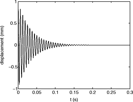

    

    Free vibration response for a single degree of freedom spring–mass–damper system

    Fig. P2.10b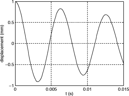

    

    First few cycles of free vibration response for a single degree of freedom spring–mass–damper system

  • (d) If the system mass is 1 kg, determine the spring constant (in N/m).

References

http://en.wikipedia.org/wiki/Linear_variable_differential_transformer
Inman D (2001) Engineering vibration, 2nd edn. Prentice Hall, Upper Saddle River
Taylor B, Kuyatt C (1994) NIST technical note 1297, 1994 edn. Guidelines for evaluating and expressing the uncertainty of NIST measurement results, National Institute of Standards and Technology, Gaithersburg
Thomson W, Dahley M (1998) Theory of vibrations with applications, 5th edn. Prentice Hall, Upper Saddle River
Author information
Authors and Affiliations
Corresponding author