Errata and Comments

Okuyama, Yoshifumi

doi:10.1007/978-1-4471-5667-3_8

Yoshifumi Okuyama²

1809 Accesses

The online version of the original chapters can be found under doi:10.1007/978-1-4471-5667-3.

You have full access to this open access chapter, Download chapter PDF

Keywords

These keywords were added by machine and not by the authors. This process is experimental and the keywords may be updated as the learning algorithm improves.

The following ‘’ letters are errata that should be corrected (or inserted).

Chapter 1: Mathematical Descriptions and Models

1.
Page 5: Eq. (1.10),
2.
Page 6: Eq. (1.18),
3.
Fig. 1.5: Time sequence of the solution for Example 1.6
4.
Below Fig. 1.5: Note that the response is delayed by one step as shown in Fig. 1.5 if (i.e., y(k)=x ₁(k−1)) is applied to the computer program for (1.55). This response corresponds to the result of Exercise (7).
5.
Page 7: Eq. (1.21),
6.
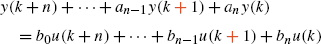
Page 13: Eq. (1.35),
7.
Page 13:
8.
Page 13: For simplicity, the initial conditions are assumed to be zero (i.e., y(0)=y(1)=⋯=y(n−1)=0 and also u(0)=u(1)=⋯=u(n−1)=0).

Comments: There would be no contradiction, because y(κ) and u(κ) in (1.35) defined for κ=k+n (κ≥n). However, in a computer simulation, backward expressions (1.19), (1.21), and (1.40) should be used.
9.
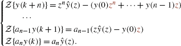
Page 13: Eq. (1.36),
10.
Page 14: Eq. (1.38), The is given as
and
11.
Page 18:
12.
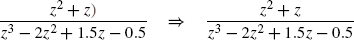
Page 18:
Tips: The z-transforms of the above equations are given as:
$$ \begin{bmatrix} z-1 & -1\\ 0.5 & z \end{bmatrix} \begin{bmatrix} \hat{x}_1(z)\\ \hat{x}_2(z) \end{bmatrix} = \begin{bmatrix} \hat{u}(z)\\ \hat{u}(z) \end{bmatrix} $$
Then,
$$\begin{bmatrix} \hat{x}_1(z)\\ \hat{x}_2(z) \end{bmatrix} = \frac{1}{z^2-z+0.5} \begin{bmatrix} z & 1\\ 0.5 & z-1 \end{bmatrix} \begin{bmatrix} z/(z-1)\\ z/(z-1) \end{bmatrix}. $$
Thus,
$$\hat{y}(z)=\hat{x}_1(z) =\frac{z^2+z}{(z^2)-z+0.5)(z-1)} =\frac{z^2+z}{z^3-2z^2+1.5z-0.5}. $$
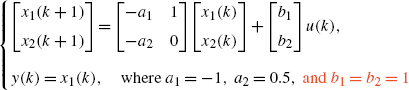
13.
Page 19: The caption in Fig. 1.6, Fig. 1.6 Block diagram for Example 1.6, where a ₁=1, , and b ₁=b ₂=1
14.
Page 23: Eq. (1.68),
15.
Page 24: In Table 1.2, The fourth line in ‘Discrete time’,
16.
Page 25: Eq. (1.76),
where
$$\boldsymbol{I}= \begin{bmatrix} 1 & 0\\ 0 & 1 \end{bmatrix} $$
17.
Page 26: Eqs. (1.78), (1.79), and (1.80), My first manuscript was written as follows:
$$\begin{cases} \boldsymbol{x}(k+1)=\boldsymbol{\Phi}(h)\boldsymbol{x}(k)+\boldsymbol{\Gamma}(h)u(k),\quad \boldsymbol{\Gamma}(h) =\int_0^h\boldsymbol{\Phi}(\tau)\boldsymbol{B}\mathrm{d}\tau\\ y(k)=\boldsymbol{Cx}(k). \end{cases} $$

$$\begin{cases} z\hat{\boldsymbol{x}}(z)=\boldsymbol{\Phi}\hat{\boldsymbol{x}}(z) +\boldsymbol{\Gamma}\hat{u}(z)\\ \hat{y}(z)=\boldsymbol{C}\hat{\boldsymbol{x}}(z). \end{cases} $$

$$\hat{y}(z)=\boldsymbol{C}[\boldsymbol{I}-\boldsymbol{\Phi}z^{-1}]^{-1}\boldsymbol{\Gamma}z^{-1}\hat{u}(z). $$
These expressions might be preferable to (1.78), (1.79), and (1.80).

Chapter 2: Discretized Feedback Systems

1.
Page 50: Eq. (2.7),
2.
Page 56: In Eq. (2.25),
3.
Page 69: Eq. (2.62),
4.
Page 71: In the last line ⋯and the problem is proved.

Chapter 3: Robust Stability Analysis

1.
Page 75: Eq. (3.8),
2.
Page 94: Eq. (3.46) in Theorem 3.3,
3.
Page 94: The verification of robust stability using the above modified Hall diagram (off-axis -circles) is based on the following theorem.

Chapter 4: Model Reference Feedback and PID Control

1.
Page 114: In Eqs. (4.16), (4.17), (4.20), and (4.21),
2.
Page 117: In Eq. (4.22),
3.
Page 117: In the first line under Fig. 12, ⋯ , characteristic equation is given as
4.
Page 132:
5.
Page 140: In Exercise (3), determine the characteristic equation , $\mathcal{F}(z)=0$, for Example 4.1 (A) ⋯ .
6.
Page 140: (4) Show that the approximate PID control system in Fig. 4.18 is obtained from the model-reference feedback system in Fig. 4.17, when $\mathcal{D}_{m}(\cdot)$ and $\mathcal{D}_{f}(\cdot)$, are .

Chapter 5: Multi-Loop Feedback Systems

1.
Page 153:
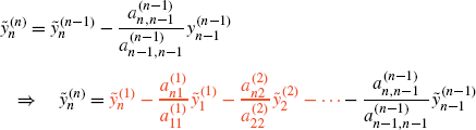
2.
Page 153: ⋯, where $y_{j}^{(j)}$ ⇒ ⋯, where $\tilde{y}_{j}^{(j)}$
3.
Page 153: ⋯all principal minors of matrix $\mathcal{A}$ ⇒ ⋯all principal minors of matrix
4.
Page 163:
5.
Page 163: ⋯, where $y_{j}^{(j)}$ ⇒ ⋯, where $\tilde{y}_{j}^{(j)}$
6.
Page 163: ⋯all principal minors of matrix $\mathcal{A}$ ⇒ ⋯all principal minors of matrix
7.
Page 177:

Chapter 6: Interval Polynomials and Robust Performance

1.
Page 186: Equation (6.17) should be written as follows:
2.
Page 191: Fig. 6.3 ⋯ for discrete control system ⇒ Fig. 6.3 ⋯ for discrete control
3.
Page 192:
The proof of Lemma 6.1 is given as follows:
$$\begin{aligned} & \qquad x^2+(y-\gamma)^2= \frac{[1-(1+\gamma^2)\theta^2]^2+[-\gamma+2\theta(1+\gamma^2) -\gamma(1+\gamma^2)\theta^2]^2}{ [1-2\gamma\theta+(1+\gamma^2)\theta^2]^2} \\ & {=}\,\frac{(1+\gamma^2)[1+(1+\gamma^2)\theta^4-2\theta^2 +4(1+\gamma^2)\theta^2+\gamma^2(1+\gamma^2)\theta^4 -4\gamma\theta-4\gamma(1+\gamma^2)\theta^3+2\gamma^2\theta^2]}{ [1-2\gamma\theta+(1+\gamma^2)\theta^2]^2} \\ & {=}\,\frac{(1+\gamma^2)[1+4\gamma^2\theta^2 +(1+\gamma^2)^2\theta^4 -4\gamma\theta-4\gamma(1+\gamma^2)\theta^3 +2(1+\gamma^2)\theta^2]}{ [1-2\gamma\theta+(1+\gamma^2)\theta^2]^2} =1+\gamma^2. \end{aligned}$$
Thus, Lemma 6.1 has been proved. □
4.
Page 204:

Chapter 7: Relation to Discrete Event Systems

1.
Page 228: Fig. 7.6 Petri net systems ⇒ Fig. 7.6 Petri net systems
2.
Page 232: In (7.21),
3.
Page 234: Their notation is ⋯ ⇒
4.
Page 234:
and
5.
Page 235: In (7.28) and (7.33),
6.
Page 236:
7.
Page 237: ⋯ and three events. ⇒ ⋯ and events.
8.
Page 239:
9.
Page 239: The equations for continuous-time systems should be corrected as follows:
and
furthermore,