Hidden Markov Model

Abstract

Real-time processes produce observations that can be discrete, continuous, stationary, time variant, or noisy. The fundamental challenge is to characterize the observations as a parametric random process, the parameters of which should be estimated, using a well-defined approach. This allows us to construct a theoretical model of the underlying process that enables us to predict the process output as well as distinguish the statistical properties of the observation itself. The hidden Markov model (HMM) is one such statistical model. HMM interprets the (nonobservable) process by analyzing the pattern of a sequence of observed symbols. An HMM consists of a doubly stochastic process, in which the underlying (or hidden) stochastic process can be indirectly inferred by analyzing the sequence of observed symbols of another set of stochastic processes. HMM comprises (hidden) states that represent an unobservable, or latent, attribute of the process being modeled. HMM-based approaches are widely used to analyze features or observations, such as usage and activity profiles and transitions between different states of the process, to predict the most probable sequence of states. The HMM is a stochastic model of discrete events and a variation of the Markov chain, a chain of linked states or events, in which the next state depends only on the current state of the system. The states of an HMM are hidden (or can only be inferred from the observed symbols). For a given model and sequence of observations, HMM is used to analyze the solution to problems related to model selection, state-sequence determination, and model training (for more details, see the section “The Three Basic Problems of HMM”).

The best thing about the future is that it comes one day at a time.

—Abraham Lincoln

These keywords were added by machine and not by the authors. This process is experimental and the keywords may be updated as the learning algorithm improves.

Real-time processes produce observations that can be discrete, continuous, stationary, time variant, or noisy. The fundamental challenge is to characterize the observations as a parametric random process, the parameters of which should be estimated, using a well-defined approach. This allows us to construct a theoretical model of the underlying process that enables us to predict the process output as well as distinguish the statistical properties of the observation itself. The hidden Markov model (HMM) is one such statistical model. HMM interprets the (nonobservable) process by analyzing the pattern of a sequence of observed symbols. An HMM consists of a doubly stochastic process, in which the underlying (or hidden) stochastic process can be indirectly inferred by analyzing the sequence of observed symbols of another set of stochastic processes. HMM comprises (hidden) states that represent an unobservable, or latent, attribute of the process being modeled. HMM-based approaches are widely used to analyze features or observations, such as usage and activity profiles and transitions between different states of the process, to predict the most probable sequence of states. The HMM can be represented as a stochastic model of discrete events and a variation of the Markov chain, a chain of linked states or events, in which the next state depends only on the current state of the system. The states of an HMM are hidden (or can only be inferred from the observed symbols). For a given model and sequence of observations, HMM is used to analyze the solution to problems related to model selection, state-sequence determination, and model training (for more details, see the section “The Three Basic Problems of HMM”).

• The fundamental theory of HMMs was developed on the basis of pioneering work by Baum and colleagues (Baum and Petrie 1966; Baum and Eagon 1967; Baum and Sell 1968; Baum et al. 1970; Baum 1972). Earlier work in this area is credited to Stratonovich (1960), who proposed an optimal nonlinear filtering model, based on the theory of conditional Markov processes. A recent contribution to the application of HMM was made by Rabiner (1989), in the formulation of a statistical method of representing speech. The author established a successful implementation of an HMM system, based on discrete or continuous density parameter distributions.

• This chapter describes HMM techniques, together with their real-life applications, in such management solutions as intrusion detection, workload optimization, and fault prediction.

Discrete Markov Process

A system may be described at any time as being in one of the states S ₁, S ₂, S _n (see Figure 5-1). When the system undergoes a change from state S _i to S _j at regular time intervals with a certain probability p _ij, this can be described by a simple stochastic process, in which the distribution of future states depends only on the present state and not on how the system arrived at the present state. The matrix P, with elements p _ij, is called the transition probability matrix of the Markov chain. In other words, we can describe a discrete Markov process as a phenomenon evolving in regularly spaced intervals, such that, for a given present state, past and future are statistically independent. Conventionally, a time-evolving phenomenon in which only the present state affects the future state, is called a dynamic system. The exclusive dependence of future states on present states allows us to model the solutions, using random variables instead of deterministic objects. A random variable defines a set of possible outcomes (the sample space Ω) and a probability distribution that associates each outcome with a probability.

Figure 5-1.

Markov chain with five states (S1–S5) with selected state transitions P(i, j)

A simple example of a discrete Markov process—a Markov chain—is a random walk in one dimension. In this case, an individual may move forward or backward with a certain probability. Formally, you can define independent random variables , where each variable is either +1 (forward movement) or −1 (backward movement), with a 50 percent probability for each value. Statistically, you may define a random walk as a sequence Q _t of random variables that increments, using independent and identically distributed (iid) random variables S, such that

where expectation E(Q _n) = 0, and variance . If is the sequence of integers, then

This equation tells us that the probability that the random walk will be at S _j at time t + 1 depends only on its current value and not on how it got there. Formally, the discrete Markov process admits three definitions, described in the following sections.

Definition 1

A Markov chain on Ω is a stochastic process {q0, q1,...,qt}, with each , such that

You construct Ω × Ω transition matrix P, whose (i, j) th entry represents , with the following properties:

A matrix P with these properties is called a stochastic matrix.

Definition 2

The (ij) th entry P ⁿ(i, j) of the matrix P ⁿ gives the probability that the Markov chain, starting in state i, will be in state j after n steps.

Definition 3

Let u ⁽⁰⁾ be the probability vector that represents the starting distribution. Then, the probability that the chain is in state j after n steps is the jth entry in the vector:

u ⁽ⁿ⁾ = u⁽⁰⁾P⁽ⁿ⁾

If you want to examine the behavior of the chain under the assumption that it starts in a certain state i, you simply choose u to be the probability vector, with ith entry equal to 1 and all other entries equal to 0. The stochastic process defined in the following sections can also be characterized as an observable Markov model, because each state can be represented as physical event.

Introduction to the Hidden Markov Model

The previous sections discussed a stochastic process characterized by a Markov model in which states correspond to an observable physical phenomenon. This model may be too restrictive to be of practical use in realistic problems in which states cannot directly correspond to a physical event. To improve its flexibility, you expand the model into one in which the observed output is a probabilistic function of a state. Each state can produce a number of outputs, according to a unique probability distribution, and each distinct output can potentially be generated at any state. The resulting model is the doubly embedded stochastic model referred to as the HMM. The underlying stochastic process in the HMM produces a state sequence that is not directly observable and that can only be approximated through another set of stochastic processes that produces the sequence of observations.

Figure 5-2 illustrates an extension of a discrete Markov process into a doubly stochastic HMM. The new HMM allows observation symbols to be emitted from each state, with a finite probability distribution. This lets the model be more expressive and flexible than the simple Markov chain. Additionally, as illustrated in Figure 5-3, you can model physical processes through a sequence of observed symbols that is true in most practical cases. The key difference from a conventional Markov chain is that, in analyzing the sequence of observed states, you cannot say exactly which state sequence produced these observations; you can, however, calculate the likelihood of a certain state sequence’s having produced them. This indicates that state sequence is hidden and can only be observed through a sequence of observed states or symbols.

Figure 5-2.

Hidden Markov model with four hidden states and three observed states

Figure 5-3.

Hidden Markov model: trellis representation

Essentials of the Hidden Markov Model

A complete specification of the HMM (Rabiner 1989) requires formal definition of the following elements:

• Number of hidden states: (N) in the model. Individual states are represented as ; the state at time t is represented as q _t.

• State transition probability distribution: , to represent state transition from state i to state j, where , . This property is similar to Definition 5-1 of a Markov chain.

• Observation symbol probability distribution: () for state j, where .

• Initial state distribution: (), where .

Once the HMM parameters are defined for a physical process by appropriate values of N, M, P, B, p, you can analyze an observation sequence (output) , in which each x _t is one of the symbols from observation matrix O at time t.

Formally, an HMM can be defined by specifying model parameters N and M, observation symbols O, and three probability matrices P, B, and p. For simplicity, you can use the compact form,

to indicate the complete parameter set of the model. The HMM described here makes two assumptions:

• Markov assumption: The current state is dependent only on the previous state; this represents the memory of the model.

• Independence assumption: Output observation o _t at time t is dependent only on the current state; it is independent of previous observations and states.

The Three Basic Problems of HMM

The preceding section described the model for HMM. This section identifies the basic problems that need to be solved to apply the model to real-world problems.

These basic problems fall into three categories:

• Problem 1. Evaluation: Given the observation sequence and an HMM model , how do we compute the probability of X? The solution to this problem allows us to select the competing model that best matches the observation sequence.

• Problem 2. Decoding: Given the observation sequence and an HMM model , how do we find the state sequence that best explains the observations? The solution to this problem attempts to uncover the hidden part of the stochastic model.

• Problem 3. Learning: How do we adjust the model parameters to maximize ? The solution to this problem attempts to optimize the model parameters to best describe the observation sequence. Furthermore, the solution allows us to adapt the model parameters, according to the observed training data sequence.

Consider the problem of failure prediction, which assesses the risk of failure in future time. In a typical system, components have underlying dependencies that allow an error to propagate from one component to another. Additionally, there exist health states that cannot be cannot be measured but that can induce errors among dependable components. These health states progress through normal performance state, subperformance state, attention-needed state, and, ultimately, failure state. It is therefore essential to identify the operational states accurately to avoid a reactive shutdown of the system. In this scenario, health states correspond to hidden states, and observations correspond to a sequence of error conditions. This lets the system administrator schedule preventive maintenance ahead of a complete system failure. Because faults are hidden (and so cannot be measured) and produce symbols corresponding to errors, you can model the problem of failure prediction to an HMM. For the sake of simplicity, you may assume that faults can be predicted by identifying unique patterns of errors that can be measured, using system counters.

Although the complete system can be modeled, using a normal state and failed states, such models do not provide component-level granularity for tracking the progression of failure through dependent components. For this reason, system architects categorize failure into multiple domains to attribute the prediction of a failure to a specific component and thus avoid a system-level catastrophic shutdown.

The first task is performed by using the solution to Problem 3, in which individual models for each failure domain () are constructed through a training process. This process assigns the HMM parameters to the descriptive model that enables an optimal match between error patterns and the corresponding transition to a fault state by the system. In a computer system this training can be supported by system event-log information, which contains error information as well as failure descriptions.

To understand the physical meaning of the model states, you identify the solution to Problem 2. In this case, the statistical properties of error counters translate into the sequence of observations occurring in each health state of the models. The definition and the number of states are dependent on the objectives and characteristics of the application. This process allows us to fine-tune the model to improve its capability to represent the various states that characterize system health. Normal state and failure state are the two end states of the HMM; intermediate states are added as needed to help predict the progression of the faulty behavior. Adding intermediate states affords modeling of predictive and critical scenarios that facilitate incorporation of repair mechanisms in anticipation of an actual failure.

Once you have the set of HMMs (Λ) designed and optimized, recognition of a component health state is performed by using the solution to Problem 1.

Solutions to the Three Basic Problems of HMM

The following sections present the solutions to the three fundamental problems of HMM. The solutions to these problems are critical to building a probabilistic framework.

Solution to Problem 1

The solution to Problem 1 involves evaluating the probability of observation sequence given the model λ; that is, . Consider a state sequence , where q ₁ and q _t are initial and final states, respectively. The probability of an observation X sequence for a state sequence Q and a model λ can be represented as

From the property of a Markov chain, you can represent the probability of the state sequence as

Summation over all possible state sequences is as follows:

Unfortunately, direct computation is not very practical, because it requires 2nN ⁿ multiplications. At every , N possible states can be reached, which turns out to be a large number. For example, at n = 100 (number of observation sequences) and N = 5 (states), there can be possible computations. Fortunately, an efficient approach, called the forward algorithm, achieves the same result.

Forward Algorithm

Consider a forward variable α _t(i) that represents the probability of a partial observation sequence up to time t, such that the underlying Markov process is in state S _i at time t, given the HMM model λ:

You can compute α _t(i) recursively via the following steps:

• 1. Initialize the forward probability as a joint probability of state S _i and initial observation x ₁. Let for 1 £ i £N.

• 2. Compute α_n(j) for all states j and t = n, using the induction procedure, substituting :

• 3. Using the results from the preceding step, compute

The total number of computations involved in evaluating the forward probability is N ² n rather than 2nN ⁿ, as required by direct computation. For n = 100 and N = 5 the total number of computations is 2,500, which is 10⁶⁹ times smaller in magnitude.

Backward Algorithm

For the forward algorithm you can also define a backward variable β_t(i) that represents the probability of a partial observation sequence from time t + 1 to the end (instead of up to t. as in the forward algorithm), where the Markov process is in state S _i at time t for a given model λ. Mathematically, you can represent the backward variable as

You can compute α _t(i) recursively via the following steps:

• 1. Define β _n(i) = 1 for 1 ≤i £N.

• 2. Compute

Scaling

A practical impediment in modeling long sequences of HMMs is the numerical scaling of conditional probabilities. Efficient computation of conditional probabilities helps in estimating the most likely sequence of states for a given model. For a sufficiently large sequence the probability of observing a long sequence tends to be so extremely small that numerical instability occurs. In most cases, the resulting computations exceed the precision range of essentially any machine (including double-precision). The most common approach for mitigating this situation is to rescale the conditional probabilities, using efficient scaling mechanisms.

For example, let’s revisit the forward variable equation,

In the case of forward variable α _t(i), you obtain the new value α _t+1(i) by multiplying by p_ij and b _j(x _t). These probabilities tend to be small and can underflow. Logarithms may not be helpful, because you are dealing with the sum of products. Furthermore, logarithms require computation of the logarithm and exponential for each addition. Basic scaling procedure multiplies α _t(i) with the scaling coefficient, with the goal of keeping the scaled α _t(i) within the dynamic precision range of the machine. At the end of computation, scaling coefficients are canceled out. The scaling coefficients need not be applied at every t-step but can be used whenever necessary.

Solution to Problem 2

Unlike the solution of Problem 1, identifying the optimal state sequence is a complex problem, because there can be many criteria. Part of the complexity originates from the definition of the measure of optimality, in which several unique criteria are possible. One solution is to identify the states q _t that are most likely to occur individually at time t. This solution attempts to maximize the expected number of correct individual states. To implement the solution to Problem 2, you define the variable γ _t(i) as the probability of being in state S _i at time t, given the observation sequence X and model λ, such that

Using the definition of conditional probability, you can express this equation as

You can rewrite Equation 5-7, using the forward-backward variable, as

where α _t(i) defines the probability of partial observation and state S _i at time t, and β _t(i) defines the remainder of the probability of observation and state S _i at time t. Using γ _t(i), you can solve for the individually most likely state at each time t by calculating the highest probability of being in state S _i at time t, as expressed by the following equation:

Although this equation maximizes the expected number of correct states by choosing the most likely state at each time interval, the state sequence itself may not be valid. For instance, in the case of the individually most likely states in the sequence q _t = S _i and q _t+1 = S_j, the transition probability p _ij may be 0 and hence not valid. This solution identifies the individually most likely state at any time t without giving any consideration as to the probability of the occurrence of the sequence of states.

One way to address this issue is to maximize the occurrence of a sequence of more than one state. This allows automatic evaluation of valid occurrences of states, while evaluating for the most likely sequence. One widely used scheme is to find the single most likely sequence of states that ultimately results in maximizing . This technique, which is based on dynamic programming, is called a Viterbi algorithm. To find the single best state sequence, you define a variable δ _t(i) that represents the highest probability along one state sequence (path) that accounts for first t observations and that ends in state S _i, as follows:

You can compute δ _t+1(j) by induction, as

from which it is clear that to retrieve the state sequence, you need to track the state that maximizes δ _i(i) at each time t. This is done by constructing an array ψ _t+1(j) that defines the state at time t from which a transition to state S _j maximizes the probability δ _t+1(j). Mathematically, this can be represented as

The complete procedure for finding the best state sequence consists of the following steps:

Initialization

Recursion

Termination

State Sequence Backtracking

The Viterbi algorithm is similar to the forward procedure, except that it uses maximization over previous states instead of a summation.

Solution to Problem 3

The solution to Problem 3 involves a method for adjusting the model parameters (P,B,π) to maximize the probability of an observation sequence for a given model. In practice there is no well-known method that maximizes the probability of observation sequence. However, you can select λ = (P,B,p), such that P(X|λ) is locally maximized, using an iterative method, such as the Baum-Welch algorithm.

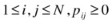
To specify the reestimation of HMM parameters, you define the variable γ _t(i,j) as the probability of being in state S _i at time t and in S _j at time t + 1 for a given model λ and observation sequence X, such that

Using the definition of the forward-backward algorithm, you can rewrite Equation 5-10 as

As defined by Equation 5-8, γ _t(i) is the probability of being in state S _i at time t, given the observation sequence and model. Using this equation, you can relate γ _t(i) to γ _t(i, j) by summing over j as

By summing γ _t(i) over time t, you can quantify the number of times state S _i is visited or, alternatively, the expected number of transitions made from state S _i. Similarly, summation of γ _t(i, j) over time t reveals the expected number of transitions from state S _i to state S _j. Given γ _t(i), γ _t(i, j), and the current model λ, you can build the method to reestimate the parameters of the HMM model (). The method can be broken down as follows:

• 1. At time t = 1 the expected frequency at state S _i is given by

• 2. The probability of transiting from state S _i to state S _j, which is the desired value of , is given by

  

  The numerator is the reestimated value of the expected number of transitions from state S _i to state S _j; the denominator is the expected number of transitions from S _i to any state.

• 3. The probability of observing symbol k, given that the model is in state S _j, is given by

  

  The numerator of the reestimated is the expected number of times the model is in state S _j with observation symbol k; the denominator is the expected number of times the model is in state S _j.

With this method, you use the current model λ(P,B,π) to reestimate the new model , as described by the previous three steps. The reestimation process is an iterative method consisting of the following steps:

• 1. Initialize l(P,B,p) with a best guess or random value, or use the existing model.

• 2. Compute α _t(i),β _t(i),γ _t(i),γ _t(i, j).

• 3. Reestimate the model .

• 4. If , repeat step 2.

The final result of this reestimation process is called the maximum likelihood estimation (MLE) of the parameters of the HMM. The forward-backward algorithm yields only the local maximum.

Continuous Observation HMM

The previous sections considered a scenario in which observations are discrete symbols from a finite alphabet, enabling use of the discrete probability density for each state in the system. For many practical implementations, however, observations are continuous vectors. Although it is possible to quantize continuous vectors via codebooks, and so on, quantization may entail degradation. Therefore, it is advantageous to have an HMM with continuous observations, whose probability density function (PDF) is evaluated as a convex combination of other distribution functions—a mixture distribution, with an associated mixture weight. The number of components is restricted to being finite. For a given pool of observations, mixture distributions are employed to make statistical inferences about the properties of the subpopulations without requiring the label identifying the subpopulation to which the observation belongs. The number of components M (subpopulations) depends on the number of observation clusters (learned through unsupervised algorithms, such as k-means) that group the pool of observations. Generally, each mixture component represents an m-dimensional categorical distribution, where each of the M possible outcomes is specified with the probability of each outcome. Each mixture component follows the similar distributions (normal, log-normal, and so on) and represents a unique qualification for classifying the set of continuous observations at any time instance as a unique symbol (similar to discrete observations). Mixture components that are trained using the EM algorithm are able to self-organize to fit a data set. The continuous observation model produces sequences of hidden clusters (or a mixture symbol) at each time step of the HMM state transition, according to a state-to-cluster-emission probability distribution. Clusters (or mixture symbols) can be considered the hidden symbols embedded in the hidden states. For example, a hidden state may represent a specific workload, and a symbol may represent a specific attribute of the workload, based resource utilization.

You start with the representation of the probability density function (PDF) that allows its parameters to be reestimated in a consistent manner. The most general form of PDF that can be used for the reestimation process is given by a multivariate normal distribution or a mixture of Gaussian distributions:

where

X = observation vector ()

M = number of mixture densities

c _jm = weight of the mth mixture in the jth state

= any elliptically symmetrical density function (e.g., a Gaussian)

μ _jm = mean vector for the mth mixture in the jth state

U _jm= covariance matrix for the mth mixture and jth state

In statistics a mixture model is a probabilistic model in which the underlying data belong to a mixture distribution. In a mixture distribution the density function is a convex combination (i.e., a linear combination in which all coefficients or weights sum to 1) of other PDFs. It can be shown (Liporace 2006; Hwang 1986) that reestimation of the coefficients for mixture density (c _jm,μ _jm,U _jm) can be represented as

where (X _t–μ _jk)^T represents the vector transpose, and ε _t(j, k), the probability of being in state j at time t with the kth mixture accounting for X _t:

The reestimation formula for p _ij is similar to that defined for discrete observation density. The reestimation formula for c _jk is the ratio of the expected number of times the system is in state j, using the kth mixture component to the expected number of times the system is in state j.

To reduce computational complexity, an alternate approach is semicontinuous HMM (SCHMM), which is a special form of continuous observation HMM (CHMM). SCHMM uses state mixture densities that are tied to a general set of mixture densities. All states share the same mixture, and only the mixture density component weights c _jk remain state-specific states.

Multivariate Gaussian Mixture Model

In the CHMM, b _j(X) is a continuous PDF that is often a mixture of multivariate Gaussian distributions of L-dimensional observations. Gaussian mixture model (GMM) density is defined as the weighted sum of Gaussian densities. The choice of the Gaussian distribution is natural and very widespread when dealing with a natural phenomenon. For the Gaussian mixture, in Equation 5-13 can be substituted by Gaussian distribution to take the mathematical form of an emission density,

Each Gaussian mixture is defined by its set of parameters, which includes the mixture distribution c _jk, the mean vectors μ _jk, and the covariance matrices U _jk. Note that a CHMM with finite mixtures of Gaussian PDFs as conditional densities is equivalent to one with simple Gaussian PDFs as conditional densities. Using a Gaussian mixture PDF, you can transform a state with a mixture density into a net of multiple single-density states. Figure 5-4 depicts a scenario in which the state S2, corresponding to a two-component mixture PDF, has been expanded into two states S2_a and S2_b with single-component PDFs and adjusted transition probabilities.

Figure 5-4.

Two-component Gaussian mixture model for state S2 expanded into single-component Gaussian model with two new states (S2_a, S2_b)

Example: Workload Phase Recognition

Recent computer architecture research has demonstrated that program execution exhibits phase behavior that can be characterized on the largest of scales (Perelman et al. 2002). In the majority of cases, workload behavior is neither homogeneous nor totally random; it is well structured, with a class of phases. As you transition between phases, you can initiate a reconfiguration by reusing configuration information for recurring phases.

Trends in datacenter and cloud computing pose interesting challenges related to power optimization and power control in a server system. A system can be represented as a set of components whose cooperative interaction produces useful work. These components may be heterogeneous in nature and may vary in their power consumption and power control mechanisms. A server system with several central processing unit (CPU), memory, and input/output (I/O) components may coordinate power control actions, using embedded controllers or special hardware. The accuracy and agility of control actions are critical in proactive tuning for performance. Observing how variations in a workload affect the power drawn by different server components provides critical data for analysis and for building models relating quality of service (QoS) expectations to power consumption. Therefore, you need an autonomous system that can extract the workload features and proactively tune the system, according to the phase of operation. The following sections present one such approach that uses performance data in a server platform to model the runtime behavior of a system. We describe a trained model that analyzes the behavioral attributes of a workload and that identifies the present and predicts with reasonable accuracy the future phase of workload characteristics, using a CHMM.

Predictive systems are devised for recognition of workload patterns and early detection of phases for characterization. The knowledge base (model) recommends appropriate actions. These systems are self-correcting and require continuous training to adapt to the previously known as well as evolutionary behavior over a period of time. The phase detection model can assist in predicting performance states and proactively adapts by tuning its parameters to meet system constraints.

Monitoring and Observations

Monitoring and measuring events from system activities is the basis for characterizing system phases and predicting the future. Modern processors have built-in performance-monitoring counters that measure real-time access patterns to processor and memory events and that help in designing analytical intelligence for a variety of dynamic decisions. Trends such as memory access patterns, rate of instruction execution, and pipeline stalls can be studied statistically for patterns, hidden correlations, and time-dependent behaviors. Measured events (resource utilization, temperature, energy consumption, performance) can be considered multiple dimensions of observed emissions. Extracted phases can be seen as predictable system characteristics, based on dynamic models that maximize the probability of the sequence of observations. Once you identify the current workload phase of operation and the most likely future phase, you can tune and provision the system with adequate resources and avoid reactive resource allocation. The CHMM-based phase characterization process uses built-in performance counters and sensors. Additionally, synthetic counters are used to abstract time-varying behavior of the workload.

Workload and Phase

Workloads are applications with specialized objectives (queries, searches, analysis, and so on) that undergo phases of execution, while operating under multiple constraints. These constraints are related to power consumption, heat generation, and QoS requirements. Optimal system operation involves complex choices, owing to a variety of degrees of freedom for power and performance parameter tuning. The process involves modeling methodology, implementation choices, and dynamic tuning. Phase detection in a workload acts as an essential ingredient, capturing time-varying behavior of dynamically adaptable systems. This ability aids in reconfiguring hardware and software ahead of variation in demand and enables reuse of trained models for recurring phases. Phase identification also helps predict future phases during workload execution, which prevents reactive response to changes in workload behavior. In this context a phase is a stage of execution in which a workload demonstrates similar power, temperature, and performance characteristics.

CHMM-assisted methodology identifies a phase’s boundaries, which are represented by a latent component of Gaussian density mixture function in the presence of system sensors and performance counters. A state’s variable can be used as a process control parameter that is fed back to the process control loop. For instance, you can feed back the workload phase (or behavioral attributes) to control thermal behavior proactively, because the physical dynamics of the temperature can be represented as a function of utilization of various system components. In general, the HMM is particularly useful, as it can exploit the underlying pattern in a sequence of events and perform state-space analysis. You may use Gaussian observations as an indicator of correctly identifying phase boundaries in a time-varying workload behavior. These phase boundaries can further be used to extract the relationship with various states of physical phenomena, such as server demand projection and thermal variation projection. Figure 5-5 for example displays a test of CPU utilization versus a workload phase that is estimated statistically at regular intervals. This function can be expanded by using more than one variable.

Figure 5-5.

CPU utilization versus phase model. The workload is composed of eight phases with phase-specific power, thermal, and performance characteristics. The red line (bottom graph) identifies the phase number that corresponds to the running average power limit (RAPL) (blue line) for each instance of workload. For example, average utilization of 65–70 percent results in phase 1

Compared with aggregate workload analysis, CHMM-assisted analysis is more accurate and informative. In general, effective tuning of system hardware and software helps in building efficient systems that minimize power and thermal dissipation for given performance constraints. Various attributes of systems can benefit from phase identification:

• For a given performance constraint, you can tune the system components (CPU, memory, I/O) for minimum power usage. Upon identifying a new phase, power is allocated (or deallocated) in a manner such that performance degradation is minimized.

• Proactive compensation for anticipated performance variation aids in avoiding reactive state changes and thus reactive latencies, improving performance.

• Available power is distributed to system components in a way that maximizes overall performance. One strategy may involve individual allocation (or deallocation), according to each component’s share in performance gain.

• Activity vectors are employed to perform thermally balanced computing, thus preventing hot spots. Activity data can also be used to coschedule tasks in a contention-free and energy-efficient manner.

• You can profile task characteristics related to (1) task priority, (2) energy and thermal profile, and (2) optimization methodology regarding latency targets proportional to task priority.

Workload phases can be exploited for adaptive architectures, guiding performance and power optimization through predictive state feedback. Because HMM uses and correlates observations with objective oriented states (such as average temperature or utilization), it may very well be a consideration in system design. Observation points can be characterized by using a reasonable set of system-wide performance counters and sensors. Hidden states that predict a control objective (such as server temperature) are measured by extracting workload phases, using feature extraction techniques. Furthermore, states share probabilistic relationships with these observations. These probabilistic relationships (also called profiles), harden and evolve with the constant use of the workload over its lifetime. If you consider a normal workload behavior to be a pattern of an observed sequence, an HMM should be appropriate for mapping such patterns to one of several states. Furthermore, it is essential to build an adaptive strategy, based on embedding numerous policies that are informed by contextual and environmental inputs. The policies govern various behavioral attributes, enhancing flexibility to maximize efficiency and performance in the presence of high levels of environmental variability. HMM-based approaches correlate the system observations (usage, activity profiles) to predict the most probable system state. HMM training, using initial data and continuous reestimation, creates a profile that consists of component models, transition probabilities, and observation symbol probabilities. CHMM aids in estimating workload phases by clustering the homogeneous behavior of multiple components. Workload phases can be interpreted by a d-dimensional Gaussian (observation vector) model of k mixtures by maximizing the probability of the sequence of observations.

Mixture Models for Phase Detection

The foremost objective of HMM-based methodology is to predict the state of the process by establishing various phase execution boundaries in the presence of time-varying behavior. Unlike traditional approaches, which study aggregate behavior, HMM-based methods can extract representative phases and workload classification, using Gaussian mixture models (GMMs). For instance, HMM can be modeled by training itself against workloads and the corresponding phases that are characterized by an inherent behavioral pattern. These phases can be considered latent symbols (as they cannot be observed directly) that are embedded in the hidden states, which, in this case, is a workload. In a trained model these latent phase patterns can be identified through sets of observed phenomena modeled through a combination of individual mixture component probability densities, along with the presence of a hidden state (evaluated using a state transition matrix). The observations exist in the form of synthetic counters and sensors that measure the performance and power characteristics of the system as well as system components. Various functional blocks that assist in workload phase detection are described in turn in the following sections.

Sensor Block

In autonomic system instrumentation, endpoints (sensors/controllers) are spread all over the platform (see Figure 5-6), and the characteristics of these endpoints can differ from one platform to another. In typical server management architecture a sensor block comprises a mix of performance counters and temperature, airflow, and power sensors. These sensors are accessed through a variety of interfaces, such as PCI Express, SMBus, PECI Bus, and CPU model specific registers (MSR). The output of the sensors is statistically processed and used as feedback. The relative importance of instrumentation may vary, according to the user requirements. In some cases, because of cost constraints, instrumentation is synthesized in lieu of physical sensors by correlating the sensor data with a different set of variables. In other cases, the instrumentation accuracy of physical sensors may vary over the operating region, outside of which it may be highly inaccurate. In such cases, sensitivity is not constant over the entire operating range of the sensor, and nonlinearity results. Nonlinearity depends on the deviation of the sensor output from the ideal behavior over the full range of the sensor. It may be necessary to calibrate the sensor within the linear operating range and then use the calibrated parameters and functions for the rest of the nonlinear operating region. Sensor data can also observe long-term drift, owing to the aging of sensor properties over a long period of time. With digital sensors, you can also have digitization error, because the measured data are an approximation of the actual data. Additionally, limitations on sampling frequency can lead to dynamic error in the measured data. The ability of an application to measure or control an aspect of the platform depends significantly on where it is hosted and its connectivity to the instrumentation endpoint.

Figure 5-6.

Instrumentation telemetry in a typical Intel Xeon server platform

Power, thermal, and performance variations in a system can result in suboptimal behavior that may need correction for platform policy compliance. This behavior must be predicted well in advance so that corrective action can be employed within a window of opportunity. Such conditions can be predicted, using a set of sensors that together can act as component Gaussians to model the overall feature density. In a platform these sensors are available as activity counters; temperature, power, and performance monitors; and so on. Classes of sensor data are as follows:

• CPU performance counters: These are special-purpose hardware counters that are built into modern microprocessors to store the counts of hardware-related activities within a CPU context. The output of these counters is used to forecast common workload behaviors, in terms of CPU utilization (cache, pipeline, idle time, stall, thermal).

• Memory performance counters: Memory performance counters identify memory access patterns, bandwidth utilization, dynamic random access memory (DRAM) power consumption, and proportions of DRAM command activity (read, write), which can be useful for characterizing the memory-intensive behavior of a workload. It is possible to characterize workload patterns by observing the proportion of read/write cycles and time in the precharge, active, and idle states.

• I/O performance counters: Three major indicators of I/O power are (1) direct memory access (DMA), (2) uncacheable access, and (3) interrupt activity. Of these the number of interrupts per cycle is the dominant indicator of I/O power. DMA indicators perform suboptimally, owing to the presence of various performance enhancements (such as write combining) in the I/O chip. I/O interrupts are typically triggered by I/O devices to indicate the completion of large data transfers. Therefore, it is possible to correlate I/O power with the appropriate device. Because this information cannot be obtained through CPU counters, it is made available by the operating system, using performance monitors.

• Thermal data: In addition to the foregoing performance counters, you may also consider using thermal data, which are available in all modern components (CPU, memory, and so on) and accessible via PECI Bus.

• Workload performance feedback: Control theoretic action initiates a defensive response, based on hysteresis, to reduce the effects of variation in resource demands. This response needs to be corrected if it interferes with the performance requirements of useful work. Excessive responses can slow down the system and negatively impact the effectiveness of the control action. State feedback communicates the optimal fulfillment of performance demands (or service-level objectives) at a given time. This feedback has to be estimated by forecasting the attributes of the fitness function that is related to the behavior of the work being performed and its dynamic requirements. Continuous state feedback trains the system-specific control actions and saves the recipe for those actions by relating it to a unique state-phase fingerprint that can repeat in the future.

Model Reduction Block

A model reduction block (MRB) is responsible for reducing the dimensionality of a dataset by retaining key uncorrelated and noncolinear datasets. This allows us to retain the most significant datasets—those that are sufficient to identify the phases of workload operation that demonstrate time-varying behavior. Input to the MRB model is time series data related to microarchitectural performance counters, workload performance counters, and analog sensors (measuring power, temperature, and so on). These data can be collected, using one of the many interfaces (PCI Express, SMBus, PECI Bus, and so on) illustrated in Figure 5-6.

You can use principal component analysis (PCA) for reducing the dimensionality of data without loss of information (see Chapter 2). The resulting output variables are the principal components, which are uncorrelated. For example, PCA transforms N inputs to M principal components , with very little information overlap . Furthermore, variance of each principal component is arranged in descending order , such that x ₁ contains the most information, and x _M, the least. Each principal component defines the dimensionality of an observation.

Emission Block

An emission block (EB) is responsible for collecting noncorrelated emissions as time series data. The raw data that are collected from sensors are noisy and have to be filtered to extract quantifiable information. The noise-reduction procedure identifies a simple dynamic system that is a good representation of the data. During the training cycle the noise reduction scheme consists of a representative distribution that fits the incoming data for a modeling window of δt. Sensor data streaming to the receiving blocks (see Figure 5-7) are delayed by a configurable time period δt. The behavior of data within the δt period is governed by the underlying equation, which is trained to reject (or reconstruct) the datapoints.

Figure 5-7.

Phase detection model, using GMM

The output of a sensor block is processed into an EB, which processes the sequence of polled sensor data to generate a continuous observation sequence. Additionally, an MRB scales down the number of sensor inputs by synthesizing those that are significant and providing independent characteristics. You may use a discrete set of weighted Gaussian PDFs, each with their own mean and covariance matrix, to enable better modeling of phase detection features, using continuous emission. The Gaussian mixture forms parametric models, whose parameters are estimated iteratively from training data, using Equations 5-14 and 5-15. In workload phase detection a d-dimensional Gaussian (independent emission) of k mixtures is modeled as a weighted sum of Gaussian densities (see Equation 5-16).

Training Block

Dynamic systems are characterized by temporal features, whose time-varying properties undergo changes during the operational period. These systems produce a temporal sequence of observations that can be analyzed for dynamic characteristics. A training block (TB) facilitates the construction of a forecast model by feeding it with metric vectors and the corresponding forecast variable for workloads with varying characteristics (such as system power). A TB performs unsupervised classification and builds data structures by partitioning the data into homogeneous clusters, such that similar objects are grouped within the same class. In the simplest case, you may use the k-means clustering algorithm, which partitions the d-dimensional emissions into k clusters, such that each emission belongs to the cluster with the nearest mean. For a given a set of emissions , the k-means clustering algorithm partitions the emissions into k sets by finding the minimum distance to observation of all the k clusters:

Each G element acts as a single-component Gaussian density function for k single-density states, each representing a distinctive workload phase; μ _i represents the mean of cluster i.

Parameter Estimation Block

You can use GMM to represent feature distributions in a workload phase prediction system, in which individual component densities model an underlying set of latent classes. A parameter estimation block (PEB) is responsible for estimating the parameters of the model λ _k that fits the data for that model. In the beginning, the model’s input data are the output sensor data from the TB, which classifies (labels) the observations as a cluster number? The classifier uses the minimum distortion, or nearest-neighbor, approach to classify the input vector, which selects the best Gaussian component from the mixture. Once the training data are buffered for each model for a time interval δt, they are used to estimate the Gaussian mixture parameters of that model. In the absence of an a priori model, a PEB initializes the number of mixtures and estimates the model parameters (c _k,μ _k,U _k). You can use the estimation maximization (EM) method, which maximizes the likelihood of the cluster-tagged data (see Chapter 1). The fundamental idea behind the EM algorithm is to introduce a variable (a Gaussian mixture component) that will simplify the maximization of likelihood. The EM algorithm is a two-step method:

• 1. E-Step: Estimate the probability distribution of each Gaussian mixture component for a given emission (X) and model (λ).

• 2. M-Step: Estimate the joint probability distribution of the data and the latent variable (Gaussian mixture component). This step modifies the model parameters of the Gaussian mixture component to maximize the likelihood of the emission and the Gaussian component itself.

Beginning with an initial model λ, the EM algorithm estimates a new model , such that . The new model then becomes the starting model for the next iteration, and the process is repeated until a convergence threshold is reached. For a given sequence of d-dimensional emission vector sequences , the a posteriori probability for the kth mixture component is given by

The formula used in reestimation of the model parameters is

This block aids in categorizing the sequence of observations to the kth Gaussian component. You can expand a single-state GCHMM into a single-density, multistate GCHMM.

Phase Prediction Model

Workload patterns that can be represented as application phases exhibit certain repetitive behaviors. You need methods to identify and predict repetitive phases to apply feasible dynamic management responses proactively. With a phase predictor block (PPB), you can estimate the observation sequence ahead of time by a configurable period δt (see Figure 5-8).

Figure 5-8.

Prediction of an observation vector for twelve phases, using an exponential smoothing function

PPB analysis is of particular interest when the workload is operating at phase boundaries, and control action has to be optimized for an anticipated phase. To build a simple prediction model, you estimate the future d-dimensional observation vectors, using the observation vector exponential smoothing model. Exponential smoothing can generally be represented as

where ,

where y _t represents the predicted output of the smoothing function at instance t –1, and x _t (our standard notation) represents the raw emission from various sensors. represents the prediction error at instance t. Exponential smoothing takes into account all past data, but the proportional contribution of older samples is diminished geometrically. This allows us to tune the value of α for two different models. In Figure 5-7 this is illustrated by the “Predict T + t” block. Figure 5-9 demonstrates the prediction process, in which a control process consumes the estimated phase signature and associates with a control action. The same action is repeated if the phase appears in the future.

Figure 5-9.

Phase prediction block; control processes use the prediction model and sensor observations to tune the process variables proactively

State Forecasting Block

In the context of workload characterization, a state represents an interesting attribute of a feedback function that, when forecasted, triggers a corrective response proactively to avoid reactive action. Reactive response lags the control action during which the function performs housekeeping and identifies the cause of behavioral change. To prevent performance degradation, you identify a key process variable that, if predicted, can generate a proactive response. A phase represents that unique behavioral characteristic of a workload that varies with time and that needs to be predicted to avoid reactive tuning.

System Adaptation

The preceding sections examined a systematic approach for detecting workload phases in dynamic systems with time-varying properties. Now, the question remains as to why we need to detect system phases.

Typically, workloads are subjected to arbitrary performance and environmental stresses, which are compensated for by using adaptive systems. Adaptation may have to serve functions that are mutually hostile and that pull in different directions. This results in needing to make compromises among solutions to maximize the fitness of the overall solution. An adaptation function will optimize power in a manner that delivers the desired performance, as perceived by the application. The desired performance may not necessarily be the highest performance. In real systems it is impossible to improve all aspects of the target policy to the same degree simultaneously. Therefore, systems develop various feedback control schemes that operate in hardware, software, or software-assisted hardware scenarios. Control objectives include

• Monitoring resource conditions in a continuous mode

• Determining how and when adaptation should be performed by modeling feedback control behavior

• Identifying real-time constraints and resource requirements for a given workload behavior

• Identifying choice of available execution paths for a given autonomic element

• Provisioning future resource requirements of a server, based on current resource usage and work behavior

• Discovering inherent phase dependencies on component power and performance tuning

The QoS profile governs an appropriate level of resource reservation by indicating the output quality levels in a dynamic fashion. In general, the QoS maximization process starts with an initial resource allocation, which it revises, according to changing application demands and satisfaction levels. In the scenarios we have described here, it is noteworthy that intelligent control action requires an understanding of workload behavior; because workload behavior is characterized by a discrete phase, you can use this information as feedback on any control loop action. Various process control applications within a system can optimize their work function by building custom learning functions that relate the phase activity to the control action. The resulting decisions steer each control loop model to train itself dynamically, based on the historical trends, with respect to quantifiable phase behaviors.

References

Baum, Leonard E. “An Equality and Associated Maximization Technique in Statistical Estimation for Probabilistic Functions of Markov Processes.” Inequalities 3 (1972): 1–8.

Baum, Leonard E., and J. A. Eagon. “An Inequality with Applications to Statistical Estimation for Probabilistic Functions of Markov Processes and to a Model for Ecology.” Bulletin of the American Mathematical Society 73, no. 3 (1967): 360–363. http://projecteuclid.org/euclid.bams/1183528841 .

Baum, Leonard E., and Ted Petrie. “Statistical Inference for Probabilistic Functions of Finite State Markov Chains.” Annals of Mathematical Statistics (1966): 1554–1563. http://projecteuclid.org/euclid.aoms/1177699147 .

Baum, Leonard E., and George Sell. “Growth Transformations for Functions on Manifolds.” Pacific Journal of Mathematics 27, no. 2 (1968): 211–227. http://projecteuclid.org/euclid.pjm/1102983899 .

Baum, Leonard E. “An Equality and Associated Maximization Technique in Statistical Estimation for Probabilistic Functions of Markov Processes.” Inequalities 3 (1972): 1–8.

Juang, Bing-Hwang, Stephen E. Levinson, and M. Mohan Sondhi. “Maximum Likelihood Estimation for Multivariate Mixture Observations of Markov Chains (Corresp.).” IEEE Transactions on Information Theory 32, no. 2 (1986): 307–309.

Liporace, L. “Maximum Likelihood Estimation for Multivariate Observations of Markov Sources.” IEEE Transactions on Information Theory 28, no. 5 (1982): 729–734.

Sherwood, Timothy, Erez Perelman, Greg Hamerly, and Brad Calder. “Automatically Characterizing Large Scale Program Behavior.” ACM SIGARCH Computer Architecture News 30, no. 5 (2002): 45–57.

Rabiner, Lawrence. “A Tutorial on Hidden Markov Models and Selected Applications in Speech Recognition.” Proceedings of the IEEE 77, no. 2 (1989): 257–286.

Stratonovich, R. L. “Conditional Markov Processes.” Theory of Probability and Its Applications 5, no. 2 (1960): 156–178.