Support Vector Machines for Classification

Abstract

This chapter covers details of the support vector machine (SVM) technique, a sparse kernel decision machine that avoids computing posterior probabilities when building its learning model. SVM offers a principled approach to problems because of its mathematical foundation in statistical learning theory. SVM constructs its solution in terms of a subset of the training input. SVM has been extensively used for classification, regression, novelty detection tasks, and feature reduction. This chapter focuses on SVM for supervised classification tasks only, providing SVM formulations for when the input space is linearly separable or linearly nonseparable and when the data are unbalanced, along with examples. The chapter also presents recent improvements to and extensions of the original SVM formulation. A case study concludes the chapter.

Science is the systematic classification of experience.

—George Henry Lewes

These keywords were added by machine and not by the authors. This process is experimental and the keywords may be updated as the learning algorithm improves.

This chapter covers details of the support vector machine (SVM) technique, a sparse kernel decision machine that avoids computing posterior probabilities when building its learning model. SVM offers a principled approach to machine learning problems because of its mathematical foundation in statistical learning theory. SVM constructs its solution in terms of a subset of the training input. SVM has been extensively used for classification, regression, novelty detection tasks, and feature reduction. This chapter focuses on SVM for supervised classification tasks only, providing SVM formulations for when the input space is linearly separable or linearly nonseparable and when the data are unbalanced, along with examples. The chapter also presents recent improvements to and extensions of the original SVM formulation. A case study concludes the chapter.

SVM from a Geometric Perspective

In classification tasks a discriminant machine learning technique aims at finding, based on an independent and identically distributed (iid) training dataset, a discriminant function that can correctly predict labels for newly acquired instances. Unlike generative machine learning approaches, which require computations of conditional probability distributions, a discriminant classification function takes a data point x and assigns it to one of the different classes that are a part of the classification task. Less powerful than generative approaches, which are mostly used when prediction involves outlier detection, discriminant approaches require fewer computational resources and less training data, especially for a multidimensional feature space and when only posterior probabilities are needed. From a geometric perspective, learning a classifier is equivalent to finding the equation for a multidimensional surface that best separates the different classes in the feature space.

SVM is a discriminant technique, and, because it solves the convex optimization problem analytically, it always returns the same optimal hyperplane parameter—in contrast to genetic algorithms (GAs) or perceptrons, both of which are widely used for classification in machine learning. For perceptrons, solutions are highly dependent on the initialization and termination criteria.

For a specific kernel that transforms the data from the input space to the feature space, training returns uniquely defined SVM model parameters for a given training set, whereas the perceptron and GA classifier models are different each time training is initialized. The aim of GAs and perceptrons is only to minimize error during training, which will translate into several hyperplanes’ meeting this requirement. If many hyperplanes can be learned during the training phase, only the optimal one is retained, because training is practically performed on samples of the population even though the test data may not exhibit the same distribution as the training set. When trained with data that are not representative of the overall data population, hyperplanes are prone to poor generalization.

Figure 3-1 illustrates the different hyperplanes obtained with SVM, perceptron, and GA classifiers on two-dimensional, two-class data. Points surrounded by circles represent the support vector, whereas the hyperplanes corresponding to the different classifiers are shown in different colors, in accordance with the legend.

Figure 3-1.

Two-dimensional, two-class plot for SVM, perceptron, and GA hyperplanes

Note SVM vs. ANN

Generally speaking, SVM evolved from a robust theory of implementation, whereas artificial neural networks (ANN) moved heuristically from application to theory.

SVM distinguishes itself from ANN in that it does not suffer from the classical multilocal minima—the double curse of dimensionality and overfitting. Overfitting, which happens when the machine learning model strives to achieve a zero error on all training data, is more likely to occur with machine learning approaches whose training metrics depend on variants of the sum of squares error. By minimizing the structural risk rather than the empirical risk, as in the case of ANN, SVM avoids overfitting.

SVM does not control model complexity, as ANN does, by limiting the feature set; instead, it automatically determines the model complexity by selecting the number of support vectors.

SVM Main Properties

Deeply rooted in the principles of statistics, optimization, and machine learning, SVM was officially introduced by Boser, Guyon, and Vapnik (1992) during the Fifth Annual Association for Computing Machinery Workshop on Computational Learning Theory. [Bartlett (1998) formally revealed the statistical bounds of the generalization of the hard-margin SVM. SVM relies on the complexity of the hypothesis space and empirical error (a measure of how well the model fits the training data). Vapnik-Chervonenkis (VC) theory proves that a VC bound on the risk exists. VC is a measure of the complexity of the hypothesis space. The VC dimension of a hypothesis H relates to the maximum number of points that can be shattered by H. H shatters N points, if H correctly separates all the positive instances from the negative ones. In other words, the VC capacity is equal to the number of training points N that the model can separate into 2^N different labels. This capacity is related to the amount of training data available. The VC dimension h affects the generalization error, as it is bounded by where w is the weight vector of the separating hyperplane and the radius of the smallest sphere R that contains all the training points, according to: . The overall error of a machine learning model consists of ε = ε_emp + ε_g, where ε_emp is the training error, and ε_g is the generalization error. The empirical risk of a model f is .

The lower bound for risk is where is the probability of his bound’s being true for any function in the class of function with VC dimension h, independent of the data distribution.

Note

There are 2^N different learning problems that can be defined, as N points can be labeled in 2^N manners as positive or negative. For instance, for three points, there are 24 different labels and 8 different classification boundaries that can be learned. Thus, the VC dimension in R ² is 3.

SVM elegantly groups multiple features that were already being proposed in research in the 1960s to form what is referred to as the maximal margin classifier. SVM borrows concepts from large-margin hyperplanes (Duda 1973; Cover 1995; Vapnik and Lerner 1963; Vapnik and Chervonenkis 1964); kernels as inner products in the feature space (Aizermann, Braverman, and Rozonoer 1964); kernel usage (Aizermann, Braverman, and Rozonoer 1964; Wahba 1990; Poggio 1990) and sparseness (Cover 1995). Mangasarian (1965) also proposed an optimization approach similar to the one adopted by SVM. The concept of slack, used to address noise in data and nonseparability, was originally introduced by Smith (1968) and was further enhanced by Bennett and Mangasarian (1992). Incorporated into SVM formulation by Cortes (1995), soft-margin SVM represents a modification of the hard-margin SVM through its adoption of the concept of slack to account for noisy data at the separating boundaries. (For readers interested in delving into the foundations of SVM, see Vapnik 1998, 1999, for an exhaustive treatment of SVM theory.)

Known for their robustness, good generalization ability, and unique global optimum solutions, SVMs are probably the most popular machine learning approach for supervised learning, yet their principle is very simple. In his comparison of SVM with 16 classifiers, on 21 datasets, Meyer, Leisch, and Hornik (2003) showed that SVM is one of the most powerful classifiers in machine learning. Since their introduction in 1992, SVMs have found their way into a myriad of applications, such as weather prediction, power estimation stock prediction, defect classification, speaker recognition, handwriting identification, image and audio processing, video analysis, and medical diagnosis.

What makes SVM an attractive machine learning framework can be summarized by the following properties:

• SVM is a sparse technique. Like nonparametric methods, SVM requires that all the training data be available, that is, stored in memory during the training phase, when the parameters of the SVM model are learned. However, once the model parameters are identified, SVM depends only on a subset of these training instances, called support vectors, for future prediction. Support vectors define the margins of the hyperplanes. Support vectors are found after an optimization step involving an objective function regularized by an error term and a constraint, using Lagrangian relaxation.¹ The complexity of the classification task with SVM depends on the number of support vectors rather than the dimensionality of the input space. The number of support vectors that are ultimately retained from the original dataset is data dependent and varies, based on the data complexity, which is captured by the data dimensionality and class separability. The upper bound for the number of support vectors is half the size of the training dataset, but in practice this is rarely the case. The SVM model described mathematically in this chapter is written as a weighted sum of the support vectors, which gives the SVM framework the same advantages as parametric techniques in terms of reduced computational time for testing and storage requirements.

• SVM is a kernel technique. SVM uses the kernel trick to map the data into a higher-dimensional space before solving the machine learning task as a convex optimization problem in which optima are found analytically rather than heuristically, as with other machine learning techniques. Often, real-life data are not linearly separable in the original input space. In other words, instances that have different labels share the input space in a manner that prevents a linear hyperplane from correctly separating the different classes involved in this classification task. Trying to learn a nonlinear separating boundary in the input space increases the computational requirements during the optimization phase, because the separating surface will be of at least the second order. Instead, SVM maps the data, using predefined kernel functions, into a new but higher-dimensional space, where a linear separator would be able to discriminate between the different classes. The SVM optimization phase will thus entail learning only a linear discriminant surface in the mapped space. Of course, the selection and settings of the kernel function are crucial for SVM optimality.

• SVM is a maximum margin separator. Beyond minimizing the error or a cost function, based on the training datasets (similar to other discriminant machine learning techniques), SVM imposes an additional constraint on the optimization problem: the hyperplane needs to be situated such that it is at a maximum distance from the different classes. Such a term forces the optimization step to find the hyperplane that would eventually generalize better because it is situated at an equal and maximum distance from the classes. This is essential, because training is done on a sample of the population, whereas prediction is to be performed on yet-to-be-seen instances that may have a distribution that is slightly different from that of the subset trained on.

SVM uses structural risk minimization (SRM) and satisfies the duality and convexity requirements. SRM (Vapnik 1964) is an inductive principle that selects a model for learning from a finite training dataset. As an indicator of capacity control, SRM proposes a trade-off between the VC dimensions, that is, the hypothesis of space complexity and the empirical error. SRM’s formulation is a convex optimization with n variables in the cost function to be maximized and m constraints, solvable in polynomial time. SRM uses a set of models sequenced in an increasing order of complexity. Figure 3-2shows how the overall model error varies with the complexity index of a machine learning model. For non- complex models, the error is high because a simple model cannot capture all the complexity of the data which results in an underfitting situation. As the complexity index increases, the error reaches its minimum for the optimal model indexed h* before it starts increasing again. For high model indices, the structure starts adapting its learning model to the training data which results in an overfitting that reduces the training error value and increases the model VC however, at the expense of a deterioration in the test error.

Figure 3-2.

Relationship between error trends and model index

Hard-Margin SVM

The SVM technique is a classifier that finds a hyperplane or a function that correctly separates two classes with a maximum margin. Figure 3-3 shows a separating hyperplane corresponding to a hard-margin SVM (also called a linear SVM).

Figure 3-3.

Hard-maximum-margin separating hyperplane

Mathematically speaking, given a set of points x _i that belong to two linearly separable classes ω₁, ω₂, the distance of any instance from the hyperplane is equal to . SVM aims to find w, b, such that the value of g(x) equals 1 for the nearest data points belonging to class ω₁ and –1 for the nearest ones of ω₂.

This can be viewed as having a margin of

whereas and .

This leads to an optimization problem that minimizes the objective function

subject to the constraint

When an optimization problem—whether minimization or maximization—has constraints in the variables being optimized, the cost or error function is augmented by adding to it the constraints, multiplied by the Lagrange multipliers.

In other words, the Lagrangian function for SVM is formed by augmenting the objective function with a weighted sum of the constraints,

where w and b are called primal variables, and λ _i’s the Lagrange multipliers.

These multipliers thus restrict the solution’s search space to the set of feasible values, given the constraints. In the presence of inequality constraints, the Karush-Kuhn-Tucker (KKT) conditions generalize the Lagrange multipliers.

The KKT conditions are

• 1. Primal constraints

• 2. Dual constraints

• 3. Complementarity slackness

• 4. Gradient of the Lagrangian (zero, with respect to primal variables)

Based on the KKT conditions,

Note

Appearing in a study by Kuhn and Tucker (1951), these conditions are also found in the unpublished master’s thesis of Karush (1939).

Since most linear programming problems come in pairs, a primal problem with n variables and m constraints can be rewritten in the Wolfe dual form with m variables and n constraints while the same solution applies for both primal and dual formulations. The duality theorem formalizes this by stating that the number of variables in one form is equal to the number of constraints in the complementary form. The complementary slackness is the relationship between the primal and dual formulation: when added to inequalities, slack variables transform them into equalities.

The dual problem of SVM optimization is to find

subject to

Note

This last constraint is essential for solution optimality. At optimality, the dual variables have to be nonnegative, as dual variables are multiplied by a positive quantity. Because negative Lagrange multipliers decrease the value of the function, the optimal solution cannot have negative Lagrange multipliers. Active or binding constraints have a corresponding nonzero multiplier, whereas nonbinding ones are zero and do not ­affect the problem solution. SVM hyperplane parameters are thus defined by the active, binding constraints, which correspond to the nonzero Lagrange multipliers, that is, the support vector.

Solving the duality of the aforementioned problem is useful for several reasons. First, even if the primal is not convex, the dual problem will always have a unique optimal solution. Second, the value of the objective function is a lower bound on the optimal function value of the primal formulation. Finally, the number of dual variables may be significantly less than the number of primal variables; hence, an optimization problem formulated in the dual form can be solved faster and more efficiently.

Soft-Margin SVM

When the data are not completely separable, as with the points marked by a X in Figure 3-4, slack variables ξ_i are introduced to the SVM objective function to allow error in the misclassification. SVM, in this case, is not searching for the hard margin, which will classify all data flawlessly. Instead, SVM is now a soft-margin classifier; that is, SVM is classifying most of the data correctly, while allowing the model to misclassify a few points in the vicinity of the separating boundary.

Figure 3-4.

A few misclassifications, as part of soft-margin SVM

The problem in primal form now is a minimization of the objective function

subject to these two constraints:

The regularization term or box constraint, C, is a parameter that varies, depending on the optimization goal. As C is increased, a tighter margin is obtained, and more emphasis is placed on minimizing the number of misclassifications. As C is decreased, more violations are allowed, because maximizing the margin between the two classes becomes the SVM aim. Figure 3-5 captures the effect of the regularization parameter, with respect to margin width and misclassification. For , fewer training points are within the margin for C ₂ than for C ₁, but the latter has a wider margin.

Figure 3-5.

The box constraint effect on SVM performance

In dual form the soft margin SVM formulation is

subject to

The soft-margin dual problem is equivalent to the hard-margin dual problem, except that the dual variable is upper bounded by the regularization parameter C.

Kernel SVM

When a problem is not linearly separable in input space, soft-margin SVM cannot find a robust separating hyperplane that minimizes the number of misclassified data points and that generalizes well. For that, a kernel can be used to transform the data to a higher-dimensional space, referred to as kernel space, where data will be linearly separable. In the kernel space a linear hyperplane can thus be obtained to separate the different classes involved in the classification task instead of solving a high-order separating hypersurface in the input space. This is an attractive method, because the overhead on going to kernel space is insignificant compared with learning a nonlinear surface.

A kernel should be a Hermitian and positive semidefinite matrix and needs to satisfy Mercer’s theorem, which translates into evaluating the kernel or Gram matrix on all pairs of data points as positive and semidefinite, forming

where ϕ(x) belongs to the Hilbert space.

In other words,

Some popular kernel functions include

• Linear kernel:

• Polynomial function:

• Hyperbolic tangent (sigmoid):

• Gaussian radial basis function (RBF):

• Laplacian radial basis function:

• Randomized blocks analysis of variance (ANOVA RB) kernel:

• Linear spline kernel in 1D:

Kernel selection is heavily dependent on the data specifics. For instance, the linear kernel—the simplest of all—is useful in large sparse data vectors. However, it ranks behind the polynomial kernel, which avoids zeroing the Hessian. The polynomial kernel is widely used in image processing, whereas the ANOVA RB kernel is usually reserved for regression tasks. The Gaussian and Laplace RBFs are general-purpose kernels that are mostly applied in the absence of prior knowledge. A kernel matrix that ends up being diagonal indicates that the feature space is redundant and that another kernel should be tried after feature reduction.

Note that when kernels are used to transform the feature vectors from input space to kernel space for linearly nonseparable datasets, the kernel matrix computation requires massive memory and computational resources, for big data.

Figure 3-6 displays the two-dimensional exclusive OR (XOR) data, a linearly nonseparable distribution in input space (upper-left) as well as in the feature space. In the latter, 16 points (for different sets) are created for the four inputs when the kernel is applied. The choice of the Gaussian RBF kernel-smoothing parameter σ ² affects the distribution of the data in the kernel space. Because the choice of parameter value is essential for transforming the data from a linearly nonseparable space to a linearly separable one, grid searches are performed to find the most suitable values.

Figure 3-6.

Two-dimensional XOR data, from input space to kernel space

The primal formulation of the kernel SVM is

subject to and

where ϕ(x_i) is such that .

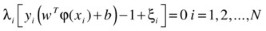
Again, the SVM solution should satisfy the KKT conditions, as follows:

• 1.
• 2.
• 3.
• 4.
• 5.
• 6.

As mentioned earlier, the dual formulation of this problem is more efficient to solve and is used in most implementations of SVM:

subject to

Note

For a dataset size of N, the kernel matrix has N ² entries. Therefore, as N increases, computing the kernel matrix becomes inefficient and even unfeasible, making SVM impractical to solve. However, ­several ­algorithms have alleviated this problem by breaking the optimization problem into a number of smaller ­problems.

Multiclass SVM

The early extensions of the SVM binary classification to the multiclass case were the work of Weston and Watkins (1999) and Platt (2000). Researchers devised various strategies to address the multiclassification problem, including one-versus-the-rest, pair-wise classification, and the multiclassification formulation, discussed in turn here.

• One-versus-the-rest (also called one-against-all [OAA]) is probably the earliest SVM multiclass implementation and is one of the most commonly used multiclass SVMs. It constructs c binary SVM classifiers, where c is the number of classes. Each classifier distinguishes one class from all the others, which reduces the case to a two-class problem. There are c decision functions: . The initial formulation of the OAA method assigns a data point to a certain class if and only if that class has accepted it, while all other classes have not, which leaves undecided regions in the feature space when more than one class accepts it or when all classes reject it. Vapnik (1998) suggested assigning data points to the class with the highest value, regardless of sign. The final label output is given to the class that has demonstrated the highest output value:

  

• Proposed by Knerr, Personnaz, and Dreyfus (1990), and first adopted in SVM by Friedman (1996) and Kressel (1999), pair-wise classification (also called one-against- one [OAO]) builds c(c – 1)/2 binary SVMs, each of which is used to discriminate two of the c classes only and requires evaluation of (c – 1) SVM classifiers. For training data from the k ^th and j ^th classes, the constraints for () are

  , for

  for

  

• The multiclassification objective function probably has the most compact form, as it optimizes the problem in a single step. The decision function is the same as that of the OAA technique. The multiclassification objective function constructs c two-class rules, and c decision functions solve the following constraints:

  .

For reasonable dataset sizes, the accuracy of the different multiclassification techniques is comparable. For any particular problem, selection of the optimal approach depends partly on the required accuracy and partly on the development and training time goals. For example, from a computational cost perspective, OAA and OAO are quite different. Let’s say, for instance, that there are c different classes of N instances and that T(N ₁) represents the time for learning one binary classifier. Using N ₁ examples, OAA will learn in cN ³, whereas OAO will require 4(c – 1)N ³/ c ².

Although the SVM parametric model allows for adjustments when constructing the discriminant function, for multiclass problems these parameters do not always fit across the entire dataset. For this reason, it is sometimes preferable to partition the data into subgroups with similar features and derive the classifier parameters separately. This process results in a multistage SVM (MSVM), or hierarchical SVM, which can produce greater generalization accuracy and reduce the likelihood of overfitting, as shown by Stockman (2010). A graphical representation of a single SVM and an MSVM is presented in Figure 3-7.

Figure 3-7.

Single multiclass SVM and MSVM flows

With a multistage approach, different kernel and tuning parameters can be optimized for each stage separately. The first-stage SVM can be trained to distinguish between a single class and the rest of the classes. At the next stage, SVM can tune a different kernel to further distinguish among the remaining classes. Thus, there will be a binary classifier, with one decision function to implement at each stage.

Hierarchical SVM as an alternative for multiclass SVM has merit in terms of overall model error. SVM accuracy approaches the Bayes optimal rule as an appropriate kernel choice and in smoothing metaparameter values. Also, by definition, for a multiclass problem with M c_i classes, and an input vector x, , because classes should cover all the search space. When the classes being considered are not equiprobable, the maximum has to be greater than 1/M; otherwise, the sum will be less than 1. Let’s say, for example, that the probability of correct classification is

where R _i is the region of the feature space in which the decision is in favor of c _i. Because of the definition of region R _i,

➩;

hence, the probability of multiclassification error is

As the number of classes M increases, P _e increases for a multiclassification flat formulation. For a hierarchical classification the multiclassification task is reduced at each stage to a binary one, with . Thus, the cumulative error for the hierarchical task is expected to converge asymptotically to a lower value than with a flat multiclassification task.

SVM with Imbalanced Datasets

In many real-life applications and nonsynthetic datasets, the data are imbalanced; that is, the important class—usually referred to as the minority class—has many fewer samples than the other class, usually referred to as the majority class. Class imbalance presents a major challenge for classification algorithms whenever the risk loss for the minority class is higher than for the majority class. When the minority data points are more important than the majority ones, and the main goal is to classify those minority data points correctly, standard machine learning that is geared toward optimized overall accuracy is not ideal; it will result in hyperplanes that favor the majority class and thus generalize poorly.

When dealing with imbalanced datasets, overall accuracy is a biased measure of classifier goodness. Instead, the confusion matrix, and the information on true positive (TP) and false positive (FP) that it holds, are a better indication of classifier performance. Referred to as matching matrix in unsupervised learning, and as error matrix or contingency matrix in fields other than machine learning, a confusion matrix provides a visual representation of actual versus predicted class accuracies.

Accuracy Metrics

A confusion matrix is as follows:

Predicted/Actual Class	Positive Class	Negative Class
Positive Class	TP	FP
Negative Class	FN	TN

Accuracy is the number of data points correctly classified by the classification algorithm:

The positive class is the class that is of utmost importance to the designer and usually is the minority class.

True positive (TP) (also called recall in some fields) is the number of data points correctly classified from the positive class.

False positive (FP) is the number of data points predicted to be in the positive class but in fact belonging to the negative class.

True negative (TN) is the number of data points correctly classified from the negative class.

False negative (FN) is the number of data points predicted to be in the negative class but in fact belonging to the positive class.

Sensitivity (also called true positive rate [TPR] or recall rate [RR]) is a measure of how well a classification algorithm classifies data points in the positive class:

Specificity (also called true negative rate [TNR]) is a measure of how well a classification algorithm classifies data points in the negative class:

Receiver operating characteristic (ROC) curves offer another useful graphical representation for classifiers operating on imbalanced datasets. Originally developed during World War II by radar and electrical engineers for communication purposes and target prediction, ROC is also embraced by diagnostic decision making. Fawcett (2006) provided a comprehensive introduction to ROC analysis, highlighting common misconceptions.

The original SVM formulation did not account for class imbalance during its supervised learning phase. But, follow-up research proposed modifications to the SVM formulation for classifying imbalanced datasets.

Previous work on SVM addressed class imbalance either by preprocessing the data or by proposing algorithmic modification to the SVM formulation. Kubat (1997) recommended balancing a dataset by randomly undersampling the majority class instead of oversampling the minority class. However, this results in information loss for the majority class. Veropoulos, Campbell, and Cristianini (1999) introduced different loss functions for the positive and negative classes to penalize the misclassification of minority data points. Tax and Ruin (1999) solved the class imbalance by using the support vector data description (SVDD), which aims at finding a sphere that encompasses the minority class and separates it from the outliers as optimally as possible. Feng and Williams (1999) suggested general scaled SVM (GS-SVM), another variation of SVM, which introduces a translation of the hyperplane after training the SVM. The translation distance is added to the SVM formulation; translation distance is computed by projecting the data points on the normal vector of the trained hyperplane and finding the distribution scales of the whole dataset (Das 2012). Chang and Lin (2011) proposed weighted scatter degree SVM (WSD-SVM), which embeds the global information in the GS-SVM by using the scatter of the data points and their weights, based on their location.

Many efforts have been made to learn imbalanced data at the level of both the data and the algorithm. Preprocessing the data before learning the classifier was done through oversampling of the minority class to balance the class distribution by replication or undersampling of the larger class, which balances the data by eliminating samples randomly from that class (Kotsiantis, Kanellopoulos, and Pintelas 2006). Tang et al. (2009) recommended the granular SVM repetitive undersampling (GSVM-RU) algorithm, which, instead of using random undersampling of the majority class to obtain a balanced dataset, uses SVM itself—the idea being to form multiple majority information granules, from which local majority support vectors are extracted and then aggregated with the minority class. Another resampling method for learning classifiers from imbalanced data was suggested by Ou, Hung, and Oyang (2006) and Napierała, Stefanowski, and Wilk (2010). These authors concluded that only when the data suffered severely from noise or borderline examples would their proposed resampling methods outperform the known oversampling methods. The synthetic minority oversampling technique (SMOTE) algorithm (Chawla et al. (2002) oversamples the minority class by introducing artificial minority samples between a given minority data point and its nearest minority neighbors. Extensions of the SMOTE algorithm have been developed, including one that works in the distance space (Koknar-Tezel and Latecki 2010). Cost-sensitive methods for imbalanced data learning have also been used. These methods define a cost matrix for misclassifying any data sample and fit the matrix into the classification algorithm (He and Garcia 2009).

Tax and Duin (2004) put forward the one-class SVM, which tends to learn from the minority class only. The one-class SVM aims at estimating the probability density function, which gives a positive value for the elements in the minority class and a negative value for everything else.

By introducing a multiplicative factor z to the support vector of the minority class, Imam, Ting, and Kamruzzaman (2006) posited that the bias of the learned SVM will be reduced automatically, without providing any additional parameters and without invoking multiple SVM trainings.

Akbani, Kwek, and Japkowicz (2004) proposed an algorithm based on a combination of the SMOTE algorithm and the different error costs for the positive and negative classes. Wang and Japkowicz (2010) also aggregated the different penalty factors as well as using an ensemble of SVM classifiers to improve the error for a single classifier and treat the problem of the skewed learned SVM. In an attempt to improve classification of imbalanced datasets using SVM standard formulation, Ajeeb, Nayal, and Awad (2013) suggested a novel minority SVM (MinSVM), which, with the addition of one constraint to the SVM objective function, separates boundaries that are closer to the majority class. Consequently, the minority data points are favored, and the probability of being misclassified is smaller.

Improving SVM Computational Requirements

Despite the robustness and optimality of the original SVM formulation, SVMs do not scale well computationally. Suffering from slow training convergence on large datasets, SVM online testing time can be suboptimal; SVMs write the classifier hyperplane model as a sum of support vectors whose number cannot be estimated ahead of time and may total as much as half the datasets. Thus, it is with larger datasets that SVM fails to deliver efficiently, especially in the case of nonlinear classification. Large datasets impose heavy computational time and storage requirements during training, sometimes rendering SVM even slower than ANN, itself notorious for slow convergence. For this reason, support vector set cardinality may be a problem when online prediction requires real-time performance on platforms with limited computational and power supply capabilities, such as mobile devices.

Many attempts have been made to speed up SVM. A survey related to SVM and its variants reveals a dichotomy between speedup strategies. The first category of techniques applies to the training phase of the SVM algorithm, which incurs a heftier computational cost in its search for the optimal separator. The intent of these algorithms is to reduce the cardinality of the dataset and speed up the optimization solver. The second category of techniques aims to accelerate the testing cycle. With the proliferation of power-conscious mobile devices, and the ubiquity of computing pushed from the cloud to these terminals, reducing the SVM testing cycle can be useful in applications in which computational resources are limited and real-time prediction is necessary. For example, online prediction on mobile devices would greatly benefit from reducing the computations required to perform a prediction.

To reduce the computational complexity of the SVM optimization problem, Platt (1998) developed the sequential minimal optimization (SMO) method, which divides the optimization problem into two quadratic program (QP) problems. This decomposition relieves the algorithm of large memory requirements and makes it feasible to train SVM on large datasets. Therefore, this algorithm grows alternately linearly and quadratically, depending on dataset size. SMO speeds up the training phase only, with no control over the number of support vectors or testing time. To achieve additional acceleration, many parallel implementations of SMO (Zeng et al. 2008; Peng, Ma, and Hong 2009; Catanzaro et al. 2008; Alham et al. 2010; Cao et al. 2006) were developed on various parallel programming platforms, including graphics processing unit (GPU) (Catanzaro et al. 2008), Hadoop MapReduce (Alham et al. 2010), and message passing interface (MPI) (Cao et al. 2006).

Using the Cholesky factorization (Gill and Murray 1974), Fine (2002) approximated the kernel matrix by employing a low-rank matrix that requires updates that scale linearly with the training set size. The matrix is then fed to a QP solver to obtain an approximate solution to the SVM classification problem. Referred to as the Cholesky product form QP, this approach showed significant training time reduction, with its approximation of the optimal solution provided by SMO. However, if the training set contains redundant features, or if the support vectors are scaled by a large value, this method fails to converge (Fine and Scheinberg 2002).

Instead of decomposing the optimization problem, Lee (2001a) reformulated the constraint optimization as an unconstrained, smooth problem that can be solved using the Newton-Armijo algorithm in quadratic time. This reformulation resulted in improved testing accuracy of the standard SVM formulation (Vapnik 1999) on several databases (Lee 2001). Furthermore, Lee (2001) argued that this reformulation allows random selection of a subset of vectors and forces creation of more support vectors, without greatly affecting the prediction accuracy of the model.

Margin vectors were identified by Kong and Wang (2010) by computing the self and the mutual center distances in the feature space and eliminating the statistically insignificant points, based on the ratio and center distance of those points. The training set was forced to be balanced, and results were compared with those found using reduced SVM (RSVM) on three datasets from the University of California, Irvine, Machine Learning Repository (Frank and Asuncion 2010). The authors found that the model resulted in better generalization performance than with RSVM but that it required slightly more training time, owing to the overhead of computing the ratios and center distances.

Zhang (2008) identified boundary vectors, using the k-nearest neighbors (k-NN algorithm. With this method the distance between each vector and all other vectors is computed, and the vectors that have among their k-NN a vector of opposing class are retained. For linearly nonseparable problems, k-NN is applied in the kernel space, where the dataset is linearly separable. The preextract boundary vectors are used to train SVM. Because this subset is much smaller than the original dataset, training will be faster, and the support vector set will be smaller.

Downs, Gates, and Masters (2002) attempted to reduce the number of support vectors used in the prediction stage by eliminating vectors from the support vector set produced by an SMO solver that are linearly dependent on other support vectors. Hence, the final support vector set is formed of all linearly independent support vectors in the kernel space obtained by using row-reduced echelon form. Although this method produced reduction for polynomial kernels, and RBF with large sigma values, the number of, support vectors reduced could not be predicted ahead of time and was dependent on the kernel and the problem.

Nguyen (2006) reduced the support vector set by iteratively replacing the two nearest support vectors belonging to the same class, using a constructed support vector that did not belong to the original training set. The algorithm was applied after training the SVM on the training set and obtaining the support vector set. The algorithm was tested on the United States Postal Service database (Le Cun 1990) and achieved significant reduction in support vector set cardinality, with little reduction in prediction accuracy.

Rizk, Mitri, and Awad (2013) proposed a local mixture–based SVM (LMSVM), which exploits the increased separability provided by the kernel trick, while introducing a one-time computational cost. LMSVM applies kernel k-means clustering to the data in kernel space before pruning unwanted clusters, based on a mixture measure for label heterogeneity. Extending this concept, Rizk, Mitri, and Awad (2014) put forward knee-cut SVM (KCSVM) and knee-cut ordinal optimization–inspired SVM (KCOOSVM), with a soft trick of ordered kernel values and uniform subsampling to reduce the computational complexity of SVM, while maintaining an acceptable impact on its generalization capability.

Case Study of SVM for Handwriting Recognition

Automated handwriting recognition (HWR) is becoming popular in several offline and online sensing tasks. Developing robust yet computationally efficient algorithms is still a challenging problem, given the increased awareness of energy-aware computing. Offline sensing occurs by optically scanning words and then transforming those images to letter code usable in the computer software environment. Online recognition automatically converts the writing on a graphics tablet or pen-based computer screen into letter code. HWR systems can also be classified as writer dependent or writer independent, with dependent systems’ having a higher recognition rate, owing to smaller variance in the provided data.

Because isolated-letter HWR is an essential step for online HWR, we present here a case study on developing an efficient writer-independent HWR system for isolated letters, using pen trajectory modeling for feature extraction and an MSVM for classification (Hajj and Awad 2012). In addition to underlining the importance of the application, this case study illustrates how stationary features are created from sequential data and how a multiclass task is converted into a hierarchical one. Usually, hidden Markov models (HMM) are better for modeling and recognizing sequential data, but with an appropriate feature generation scheme, an SVM model can be used to model variable sequence length for moderate handwriting vocabularies.

The proposed HWR workflow is composed of preprocessing; feature extraction; and a hierarchical, three-stage classification phase.

Preprocessing

The UJIpenchars database can be transformed into a sequence of points suitable for feature extraction in a way similar to preprocessing performed a step typically found in many HWR systems. The preprocessing comprises correcting the slant; normalizing the dimensions of the letter; and shifting the coordinates, with respect to the center of mass.

To correct the slant, the input, consisting of a sequence of collected points, is first written in the form of a series of vectors with polar coordinates, and then only vectors with an angle equal to or less than 50 degrees with the vertical are considered. The slant is computed by averaging the angles of the significant vectors. Next, the letter is rotated by the slant angle, and the data are normalized so that all letters have the same dimensions. Finally, the shifting of the coordinates, with respect to the center of mass, fits the letter into a square of unit dimension with a centroid with the coordinates (0, 0).

Figure 3-8 shows two letters before (left) and after (right) the preprocessing stage.

Figure 3-8.

Examples of letters before (left) and after (right) preprocessing

Feature Extraction

To obtain different representations of the letters, a set of feature vectors of fixed length should be computed. The preprocessed data, consisting of strokes of coordinate pairs [x(t), y(t)], can be modeled, using a pen trajectory technique (Jaeger 2008), and the set of features is obtained after averaging the following functions:

• Writing direction: Defined by

• where Δx, Δy, and Δs are defined as

• Curvature: Defined by the sine and cosine of the angle defined by the points (x(t - 2), y(t - 2)); (x(t), y(t)); and (x(t + 2), y(t + 2)). Curvature can be calculated from the writing direction, using the following equations:

• Aspect of the trajectory: Computed according to the equation

• Curliness: Describes the deviation of the points from a straight line formed by the previous and following points in the sequence by the equation

• where L(t) represents the length of the trajectory from point (x(t - 1), y(t - 1)) to point (x(t + 1), y(t + 1)).

In addition to the previous functions, the following global features are computed:

• Linearity: Measured by the average distance from each point of the sequence to the straight line joining the first and last points in the sequence:

• Slope of the sequence: Measured by the cosine and sine of the angle formed by the straight line joining the first and last points in the sequence and a horizontal line.

• Ascenders and descenders: Describes the number of points of the sequence below (descenders) or above (ascenders) the baseline (the straight horizontal line on which the letter is written), each weighted by its distance to the baseline.

• Variance of coordinates (for both dimensions): Measures the expansion of the points around the center of mass.

• Ratio of variances: Represents the proportion of the width to the height of the letter.

• Cumulative distance: The sum of the length of the segments of line joining consecutive points of the sequence.

• Average distance to the center, The mean of the distances from each point of the sequence to the center of mass of the letter.

Hierarchical, Three-Stage SVM

After the preprocessing and feature extraction stages, a three-stage classifier recognizes one of the 52 classes (26 lowercase and 26 uppercase letters).

• Using a binary SVM classifier, the first stage classifies the instance as one of two classes: uppercase or lowercase letter.

• Using OAA SVM, the second stage classifies the instance as one of the manually determined clusters shown in Table 3-1.

  Table 3-1. Lower- and Uppercase Clusters

• Using OAA SVM, with a simple majority vote, the third stage identifies the letter as one of the 52 classes (or subclusters). Figure 3-9 displays the hierarchy of the three-stage system.

  Figure 3-9.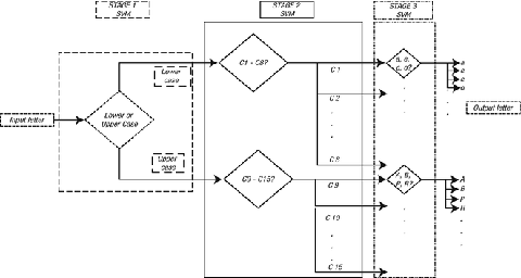

  

  Hierarchical, three-stage SVM

Experimental Results

Experimental results, implemented with the MATLAB R2011a SVM toolbox, showed (using a four-fold cross-validation) an average accuracy of 91.7 percent—or, an error rate of 8.3 percent, compared with an error rate of 10.85 percent, using 3NN (Prat et al. 2009). The three stages of the classifier achieved, respectively, 99.3 percent, 95.7 percent, and 96.5 percent accuracy. The kernel used for the three stages was an RBF with parameters tuned using a grid search algorithm. Our proposed preprocessing helped improve the general accuracy of the recognizer by approximately 1.5 percent to 2 percent.

Figure 3-10presents a confusion histogram demonstrating the occurrence of the predicted classified labels, along with their true labels. For example, in the first column, of the six letter a’s, five were correctly recognized, and one was mistaken for c. Generally, no particular trend was observed in this confusion matrix, and the error may be assumed to be randomly distributed among all classes.

Figure 3-10.

Confusion plot for classified label versus true label

Because a flat SVM architecture may seem computationally less expensive, it was compared with the proposed three-stage SVM, using OAO and OAA SVM techniques. Table 3-2 shows the recognition rates obtained using the proposed architecture, compared with a flat SVM technique as well as the3NN algorithm. The accuracy attained ranged from 65 percent, using OAA, to 82 percent, using OAO, whereas the hierarchical SVM structure reached 91.7 percent. This is due to the fact that, with a three-stage SVM, both the metaparameters of SVM (i.e., the regularization parameter between the slack and hyperplane parameters) and the kernel specifics can be better modified independently during each phase of training and better tailored to the resulting data subsets than a flat SVM model can be for the whole dataset.

Table 3-2. Recognition Rate Comparison

Complexity Analysis

Tables 3-3 and 3-4, respectively, provide the required operations for the preprocessing and feature extraction stages of the three-stage SVM, where a letter is represented by a sequence of strokes of length N, with M being the number of significant vectors, and K, the data size.

Table 3-3. Required Operations for the Preprocessing Stage

Table 3-4. Required Operations for the Feature Extraction Stage

Table 3-5 compares the required operations for the classification process using three-stage SVM and the 3NN algorithm . Both SVM optimal hyperplane coefficients and support vectors were computed during the training process. Given an input pattern represented by a multidimensional (11) vector x and a w vector representing the decision boundary (hyperplane), the decision function for the classification phase is reduced to a sign function.

Table 3-5. Comparison of Three-Stage SVM and 3NN Classifiers

The online classification task is much costlier using a 3NN classifier compared with a hierarchical SVM. In fact, every classification task requires the Euclidian distance calculation to all points in the dataset, which would be an expensive cost to incur in the presence of a large dataset. Additionally, with the lack of a classification model, the k-NN technique is a non parametric approach and requires access to all the data each time an instance is recognized. With SVM, in contrast, separating class boundaries is learned offline, during the training phase, and at runtime the computational cost of SVM training is not present. Only preprocessing, feature extraction, and a simple multiplication operation with the hyperplane parameters are involved in the online testing process. An advantage of 3NN, however, is that no training is required, as opposed to the complex SVM classification step.

References

Aizerman, M., E. Braverman, and L. Rozonoer. “Theoretical Foundations of the Potential Function Method in Pattern Recognition Learning.” Automation and Remote Control 25 (1964): 821–837.

Ajeeb, N., A. Nayal, and M. Awad. “Minority SVM for Linearly Separable and Imbalanced Datasets.” In IJCNN 2013: Proceedings of the 2013 International Joint Conference on Neural Networks, 1–5. Piscataway, NJ: Institute for Electrical and Electronics Engineers, 2013.

Akbani, Rehan, Stephen Kwek, and Nathalie Japkowicz. “Applying Support Vector Machines to Imbalanced Datasets.” In Machine Learning: ECML 2004: 15th European Conference on Machine Learning, Pisa, Italy, September 2004, edited by Jean-François Boulicaut, Floriana Esposito, Fosca Giannotti, and Dino Pedreschi, 39–50. Berlin: Springer, 2004.

Alham, N. K., Maozhen Li, S. Hammoud, Yang Liu, and M. Ponraj. “A Distributed SVM for Image Annotation.” In FSKD 2010: Proceedings of the Seventh International Conference on Fuzzy Systems and Knowledge Discovery, edited by Maozhen Li, Qilian Liang, Lipo Wang and Yibin Song, 2983–2987. Piscataway, NJ: Institute of Electrical and Electronics Engineers, 2010.

Aronszajn, N. “Theory of Reproducing Kernels.” Transactions of the American Mathematical Society 68, no. 3 (1950): 337–404.

Bartlett, P. and J. Shawe-Taylor, “Generalization Performance of Support Vector Machines and Other Pattern Classifiers”, Advances in Kernel Methods: Support Vector Learning, 1999.

Ben-Hur, Asa, and Jason Weston. “A User’s Guide to Support Vector Machines.” Data Mining Techniques for Life Sciences, edited by Oliviero Carugo and Frank Eisenhaber, 223-239. New York: Springer, 2010.

Bennett, Kristen P., and O. L. Mangasarian. “Robust Linear Programming Discrimination of Two Linearly Inseparable Sets.” Optimization Methods and Software 1, no. 1: (1992): 23–34.

Boser, Bernard E., Isabelle M. Guyon, and Vladimir N. Vapnik. “A Training Algorithm for Optimal Margin Classifiers.” In COLT ’92: Proceedings of the Fifth Annual Workshop on Computational Learning Theory, edited by David Haussler, 144–152. New York: ACM, 1992.

Cao, L. J., S. S. Keerthi, Chong-Jin Ong, J. Q. Zhang, U. Periyathamby, Xiu Ju Fu, and H. P. Lee. “Parallel Sequential Minimal Optimization for the Training of Support Vector Machines.” IEE Transactions on Neural Networks 17, no. 4 (2006): 1039–1049.

Catanzaro, Bryan Christopher, Narayanan Sundaram, and Kurt Keutzer. “Fast Support Vector Machine Training and Classification on Graphics Processors.” In ICML ’08: Proceedings of the 25th International Conference on Machine Learning, edited by William Cohen, Andrew McCallum, and Sam Roweis, 104–111. New York: ACM, 2008.

Chang, Chih-Chung, and Chih-Jen Lin. “LIBSVM: A Library for Support Vector Machines,” in “Large-Scale Machine Learning,” edited by Huan Liu and Dana Nau, special issue, ACM Transactions on Intelligent Systems and Technology 2, no. 3 (2011).

Chawla, Nitesh V., Kevin W. Bowyer, Lawrence O. Hall, and W. Philip Kegelmeyer. “SMOTE: Synthetic Minority Over-Sampling Technique.” Journal of Artificial Intelligence Research 16 (2002): 321–357.

Cover, Thomas M. “Geometrical and Statistical Properties of Systems of Linear Inequalities with Applications in Pattern Recognition.” IEEE Transactions on Electronic Computers 14 (1995): 326–334.

Das, Barnan. “Implementation of SMOTEBoost Algorithm Used to Handle Class Imbalance Problem in Data,” 2012. www.mathworks.com/matlabcentral/fileexchange/37311-smoteboost .

Downs, Tom, Kevin E. Gates, and Annette Masters. “Exact Simplification of Support Vector Solutions.” Journal of Machine Learning Research 2 (2002): 293–297.

Duda, Richard O., and Peter E. Hart. Pattern Classification and Scene Analysis. New York: Wiley, 1973.

Fawcett, Tom. “An Introduction to ROC Analysis. “Pattern Recognition Letters 27 (2006): 861–874.

Feng, Jianfeng, and P. Williams. “The Generalization Error of the Symmetric and Scaled Support Vector Machines.” IEEE Transactions on Neural Networks 12, no. 5 (1999): 1255–1260.

Fine, Shai, and Katya Scheinberg. “Efficient SVM Training Using Low-Rank Kernel Representations.” Journal of Machine Learning Research 2 (2002): 243–264.

Fisher, Marshall L. “The Lagrangian Relaxation Method for Solving Integer Programming Problems. “Management Science 50, no. 12 (2004):1861–1871.

Frank, A., and A. Asuncion. University of California, Irvine, Machine Learning Repository. Irvine: University of California, 2010. www.ics.uci.edu/`mlearn/MLRepository.html .

Friedman, J. “Another Approach to Polychotomous Classification.” Technical report, Stanford University, 1996.

Hajj, N., and M. Awad.” Isolated Handwriting Recognition via Multi-Stage Support Vector Machines.” In Proceedings of the 6th IEEE International Conference on Intelligent Systems,” edited by Vladimir Jotsov, Krassimir Atanassov, 152–157. Piscataway, NJ: Institute for Electrical and Electronic Engineers, 2012.

He, Heibo, and Edwardo A. Garcia. “Learning from Imbalanced Data.” IEEE Transactions on Knowledge and Data Engineering 21, no. 9(2009):1263–1284.

Gill, Philip E., and Walter Murray. “Newton-Type Methods for Unconstrained and Linearly Constrained Optimization.” Mathematical Programming 7 (1974): 311–350.

Imam, Tasadduq, Kai Ming Ting, and Joarder Kamruzzaman. “z-SVM: An SVM for Improved Classification of Imbalanced Data.” In AI 2006: Advances in Artificial Intelligence; Proceedings of the 19th Australian Joint Conference on Artificial Intelligence, Hobart, Australia, December 4–8, 2006, edited by Abdul Sattar and Byeong-Ho Kang, 264–273, 2006. Berlin: Springer, 2006.

S. Jaeger, S. Manke, J. Reichert, A. Waibel, “Online Handwriting Recognition: the NPen++ Recognizer”, International Journal on Document Analysis and Recognition, vol.3, no.3, 169-180, March 2008.

Jin, A-Long, Xin Zhou, and Chi-Zhou Ye. “Support Vector Machines Based on Weighted Scatter Degree.” In Artificial Intelligence and Computational Intelligence: Proceedings of the AICI Third International Conference, Taiyuan, China, September 24–25, 2011, Part III, edited by Hepu Deng, Duoqian Miao, Jingsheng Lei, and Fu Lee Wang, 620–629. Berlin: Springer, 2011.

Karush, William. “Minima of Functions of Several Variables with Inequalities as Side Constraints.” Master’s thesis, University of Chicago, 1939.

Knerr, S., L. Personnaz, and G. Dreyfus. “Single-Layer Learning Revisited: A Stepwise Procedure for Building and Training a Neural Network.” In Neurocomputing: Algorithms, Architectures and Applications; NATO Advanced Workshop on Neuro-Computing, Les Arcs, Savoie, France, 1989, edited by Françoise Fogelman Soulié and Jeanny Hérault, 41–50. Berlin: Springer, 1990.

Koknar-Tezel, S., and L. J. Latecki. “Improving SVM Classification on Imbalanced Data Sets in Distance Spaces.” In ICDM ’09: Proceedings of the Ninth IEEE International Conference on Data Mining, edited by Wei Wang, Hillol Kargupta, Sanjay Ranka, Philip S. Yu, and Xindong Wu, 259–267. Piscataway, NJ: Institute for Electrical and Electronics Engineers, 2010.

Kong, Bo, and Hong-wei Wang. “Reduced Support Vector Machine Based on Margin Vectors.” In CiSE 2010 International Conference on Computational Intelligence and Software Engineering,” 1–4. Piscataway, NJ: Institute for Electrical and Electronic Engineers, 2010.

Kotsiantis, Sotiris, Dimitris Kanellopoulos, and Panayiotis Pintelas. “Handling Imbalanced Datasets: A Review.”GESTS International Transactions on Computer Science and Engineering 30, no. 1 (2006): 25–36.

Kressel, Ulrich H.-G. “Pairwise Classification and Support Vector Machines.” In Advances in Kernel Methods: Support Vector Learning, edited by Bernhard Schölkopf, Christopher J. C. Burges, and Alexander J. Smola, 255–268. Cambridge, MA: Massachusetts Institute of Technology Press, 1999.

Kuhn, H. W., and A. W. Tucker. “Nonlinear Programming.” In Proceedings of the Second Berkeley Symposium on Mathematical Statistics and Probability, edited by Jerzy Neyman, 481–492. Berkeley: University of California Press, 1951.

Le Cun, Y., B. Boser, J. S. Denker, D. Henderson, R. E. Howard, W. Hubbard and L. D. Jackel. “Handwritten Digit Recognition with a Back-Propagation Network.” In Advances in Neural Information Processing Systems, edited by D. S. Touretzky, 396–404. San Mateo, CA: Morgan Kaufmann, 1990.

Lee, Yuh-Jye, and O. L. Mangasarian. “SSVM: A Smooth Support Vector Machine for Classification.” Computational Optimization and Applications 20 (2001a): 5–22.

Lee, Yuh-Jye, and Olvi L. Mangasarian. “RSVM: Reduced Support Vector Machines.” In Proceedings of the First SIAM International Conference on Data Mining, edited by Robert Grossman and Vipin Kumar, 5–7. Philadelphia: Society for Industrial and Applied Mathematics, 2001b .

Liu, Xin, and Ying Ding. “General Scaled Support Vector Machines.” In ICMLC 2011: Proceedings of the 3rd International Conference on Machine Learning and Computing. Piscataway, NJ: Institute of Electrical and Electronics Engineers, 2011.

Mangasarian, O. L. “Linear and Nonlinear Separation of Patterns by Linear Programming.” Operations Research 13, no. 3 (1965): 444–452.

Meyer, David, Friederich Leisch, and Kurt Hornik.” The Support Vector Machine Under Test.” Neurocomputing 55, nos. 1–2 (2003): 169–186.

Napierała, Krystyna, Jerzy Stefanowski, and Szyman Wilk. “Learning from Imbalanced Data in Presence of Noisy and Borderline Examples.” In Rough Sets and Current Trends in Computing: Proceedings of the 7th RSCTC International Conference, Warsaw, Poland, June 2010,edited by Marcin Szczuka, Marzena Kryszkiewicz, Sheela Ramanna, Richard Jensen, and Qinghua Hu, 158–167. Berlin: Springer, 2010.

Nguyen, Duc Dung, and Tuo Bao Ho. “A Bottom-Up Method for Simplifying Support Vector Solutions.” IEEE Transactions on Neural Networks. 17, no. 3 (2006): 792–796.

Ou, Yu-Yen, Hao-Geng Hung, and Yen-Jen Oyang, “A Study of Supervised Learning with Multivariate Analysis on Unbalanced Datasets.” In IJCNN ’06: Proceedings of the 2006 International Joint Conference on Neural Networks, 2201–2205. Piscataway, NJ: Institute for Electrical and Electronic Engineers, 2006.

Peng, Peng, Qian-Lee Ma, and Lei-Ming Hong. “The Research of the Parallel SMO Algorithm for Solving SVM.” In ICMLC 2009: Proceedings of the 2009 International Conference on Machine Learning and Cybernetics, 1271–1274. Piscataway, NJ: Institute for Electrical and Electronics Engineers, 2009.

Platt, John C. “Sequential Minimal Optimization: A Fast Algorithm for Training Support Vector Machines.” Technical report MSR-TR-98-14, 1998.

Platt, John C., Nello Cristianini, and John Shawe-Taylor. “Large Margin DAGs for Multiclass Classification.” In Advances in Neural Information Processing Systems 12 (NIPS ‘99), edited S. A. Solla, T. K. Leen, and K.-R. Müller, 547–553. Cambridge, MA: Massachusetts Institute of Technology Press, 2000.

Poggio, Tomaso, and Federico Girosi. “Networks for Approximation and Learning.” Proceedings of the IEEE 78, no. 9 (1990): 1481–1497.

Prat, Federico, Andrés Marzal, Sergio Martín, Rafael Ramos-Garijo, and María José Castro. “A Template-Based Recognition System for On-line Handwritten Characters.” Journal of Information Science and Engineering 25 (2009): 779–791.

Rizk, Y., N. Mitri, and M. Awad. “A Local Mixture Based SVM for an Efficient Supervised Binary Classification.” In IJCNN 2013: Proceedings of the International Joint Conference on Neural Networks, 1–8. Piscataway, NJ: Institute for Electrical and Electronics Engineers, 2013.

Rizk, Y., N. Mitri, and M. Awad. “An Ordinal Kernel Trick for a Computationally Efficient Support Vector Machine.” In IJCNN 2014: Proceedings of the 2014 International Joint Conference on Neural Networks, 3930–3937. Piscataway, NJ: Institute for Electrical and Electronics Engineers, 2014.

Schölkopf, B., John C. Platt, John C. Shawe-Taylor, Alex J. Smola, and Robert C. Williamson. “Estimating the Support of a High-Dimensional Distribution.” Neural Computation 13, no. 7 (2001):1443–1471.

Smith, F. W. “Pattern Classifier Design by Linear Programming.” IEEE Transactions on Computers, C-17. no. 4 (1968): 367–372.

Stockman, M., and M. Awad. “Multistage SVM as a Clinical Decision Making Tool for Predicting Post Operative Patient Status.” IKE ’10: Proceedings of the 2010 International Conference on Information and Knowledge Engineering. Athens, GA: CSREA, 2010.

Suykens, J. A. K. Suykens, and J. Vandewalle. “Least Squares Support Vector Machine Classifiers.” Neural Processing Letters 9, no. 3 (1999): 293–300.

Tang, Yuchun, Yan-Qing Zhang, Nitesh V. Chawla, and Sven Krasser. “SVMs Modeling for Highly Imbalanced Classification.” Journal of Latex Class Files 1, no. 11 (2002). www3.nd.edu/∼dial/papers/SMCB09.pdf.

Tang, Yuchun, Yan-Qing Zhang, N. V. Chawla, and Sven Krasser. “SVMs Modeling for Highly Imbalanced Classification.” Systems, Man, and Cybernetics B: IEEE Transactions on Cybernetics 39, no. 1 (2009): 281–288.

Tax, David M. J., and Robert P. W. Ruin. “Support Vector Domain Description.” Pattern Recognition Letters 20 (1999): 1191–1199.

Tax, David M. J., and Robert P. W. Duin. “Support Vector Data Description.” Machine Learning 54 (2004): 45–66.

Vapnik, Vladimir N. The Nature of Statistical Learning Theory. New York: Springer, 1995.

Vapnik, Vladimir N. Statistical Learning Theory. New York: Wiley, 1998.

Vapnik, Vladimir N. The Nature of Statistical Learning Theory, Second Edition. New York: Springer, 1999.

Vapnik, V., and A. Chervonenkis. “A Note on One Class of Perceptrons.” Automation and Remote Control 25 (1964).

Vapnik, V., and A. Lerner. “Pattern Recognition Using Generalized Portrait Method.” Automation and Remote Control 24 (1963): 774–780.

Veropoulos, K., C. Campbell, and N. Cristianini. “Controlling the Sensitivity of Support Vector Machines.” In IJCAI ‘99: Proceedings of the 16th International Joint Conference on Artificial Intelligence, edited by Thomas Dean, 55–60. San Francisco: Morgan Kaufmann, 1999.

Wahba, Grace. Spline Models for Observational Data. CBMS-NSF Regional Conference Series in Applied Mathematics 59. Philadelphia: Society for Industrial and Applied Mathematics, 1990.

Wang, Benjamin X., and Nathalie Japkowicz. “Boosting Support Vector Machines for Imbalanced Data Sets.” Knowledge and Information Systems 25, no. 1 (2010): 1–20.

Weston, J., and C. Watkins. Support Vector Machines for Multi-Class Pattern Recognition. In ESANN 1999: Proceedings of the 7th European Symposium on Artificial Neural Networks, Bruges, Belgium, 21–23 April 1999, 219–224. 1999. https://www.elen.ucl.ac.be/Proceedings/esann/esannpdf/es1999-461.pdf .

Zeng, Zhi-Qiang, Hong-Bin Yu, Hua-Rong Xu, Yan-Qi Xie, and Ji Gao. “Fast Training Support Vector Machines Using Parallel Sequential Minimal Optimization.” In ISKE 2008: Proceedings of the 3rd International Conference on Intelligent System and Knowledge Engineering, edited by Shaozi Li, Tianrui Li, and Da Ruan, 997–1001. Piscataway, NJ: Institute for Electrical and Electronics Engineers, 2008.

Zhang, Li, Ning Ye, Weida Zhou, and Licheng Jiao. “Support Vectors Pre-Extracting for Support Vector Machine Based on K Nearest Neighbour Method.” In ICIA 2008: Proceedings of the 2008 International Conference on Information and Automation, 1353–1358. Piscataway, NJ: Institute of Electrical and Electronics Engineers, 2008.

Zhang, Xuegong. “Using Class-Center Vectors to Build Support Vector Machines.” Neural Networks for Signal Processing IX: Proceedings of the 1999 IEEE Signal Processing Society Workshop, edited by Yu-Hen Hu, Jan Larsen, Elizabeth Wilson, and Scott Douglas, 3–11. Piscataway, NJ: Institute for Electrical and Electronic Engineers, 1999.

Zhuang, Ling, and Honghua Dai. “Parameter Optimization of Kernel-Based One-Class Classifier on Imbalance Text Learning.” Journal of Computers 1, no. 7 (2006): 32–40.