Continuous, Semi-discrete, and Fully Discretised Navier-Stokes Equations

Abstract

The Navier-Stokes equations are commonly used to model and to simulate flow phenomena. We introduce the basic equations and discuss the standard methods for the spatial and temporal discretisation. We analyse the semi-discrete equations – a semi-explicit nonlinear DAE – in terms of the strangeness index and quantify the numerical difficulties in the fully discrete schemes, that are induced by the strangeness of the system. By analysing the Kronecker index of the difference-algebraic equations, that represent commonly and successfully used time stepping schemes for the Navier-Stokes equations, we show that those time-integration schemes factually remove the strangeness. The theoretical considerations are backed and illustrated by numerical examples.

Appendices

Appendix 1: Strangeness Index of Eq. (3.1)

We analyse in detail the strangeness index of the DAE (3.1); see [39, Def. 4.4] for the precise definition. Note that we do not ask for any assumptions on the nonlinearity K and that we allow the matrix B to be rank-deficient. This then also implies that the differentiation index of (3.1) equals 2 if it is well-defined, i.e., if B is of full rank.

1.1 Linear Case

Considering any linearisation of the Navier-Stokes equations, i.e., K(u) = Ku in (3.1), we deal with the matrix pair

Following [39, Th. 3.11], we can construct a to (E, A) (globally) equivalent pair $(\tilde E, \tilde A )$ of the form

with $A_{13} \in \mathbb {R}^{b,m}$ being of full rank. Thus, the original system (3.1) is equivalent to a system of the form

$$\displaystyle \begin{aligned} \dot x_1 = A_{12}x_2 + A_{13}x_3 + f_1, \qquad \dot x_2 = A_{23}x_3 + f_2, \qquad 0 = x_1 + f_3, \qquad 0 = f_4 \end{aligned}$$

with dimensions $x_1(t)\in \mathbb {R}^{b}$, $x_2(t)\in \mathbb {R}^{n-b}$, $x_3(t)\in \mathbb {R}^{m}$. Since we have a differential and an algebraic equation for x ₁ (this causes the ‘strangeness’), we use the derivative of 0 = x ₁ + f ₃ in order to eliminate $\dot x_1$ in the first equation. Hence, we consider the pair (E _mod, A _mod) with

Since A ₁₃ is of full rank, one can show that system (E _mod, A _mod) is strangeness-free, cf. the calculation in [39, Th. 3.7]. Since we have obtained a strangeness-free system with only one differentiation, system (3.1) has strangeness index one.

1.2 Nonlinear Case

The general form of a nonlinear DAE is given by

$$\displaystyle \begin{aligned} F(t, x, \dot x) = 0. \end{aligned}$$

In regard of system (3.1) we set x := [q ^T, p ^T]^T and define

with

In the sequel we show that (3.1) has strangeness index 1 also in the nonlinear case. For this, we assume that B has full rank such that there are no vanishing equations and the pressure variable is uniquely defined. In the case $\operatorname {\mathrm {rank}} B = b < m$, we consider the following transformation.

Let $C_0\in \mathbb {R}^{m, m-b}$ be the matrix of full rank satisfying B ^T C ₀ = 0. Furthermore, $C'\in \mathbb {R}^{m, b}$ defines any matrix such that $C = [C_0\ C'] \in \mathbb {R}^{m, m}$ is invertible. With this, we obtain the relation

with $\tilde B \in \mathbb {R}^{b, n}$ having full rank. With the matrix C in hand, we first introduce the new pressure variable $\tilde p := C^{-1}p$. Thus, we consider the pair $z := [q^T, \tilde p^T]^T$. As a second step, we multiply equation (3.1) by the block-diagonal matrix diag(I _n, C ^T) from the left. In total, this yields the equivalent DAE

Note that the constraint contains (m − b) consistency equations of the form 0 = g ₁. Assuming that system (3.1) is solvable, we suppose that these are in fact vanishing equations. Thus, they have no influence on the index of the system. Furthermore, the first (m − b) components of the transformed pressure $\tilde p$ do not influence the system. These components are underdetermined and may be omitted, again without changing the index. Leaving out the underdetermined parts as well as the vanishing equations, we obtain a system of the form (3.1) with a full rank matrix B.

In the sequel, we assume that $\operatorname {\mathrm {rank}} B = m$ and show that [39, Hyp. 4.2] is satisfied for μ = 1. Note that this hypothesis is not satisfied for μ = 0, i.e., the system is not strangeness-free. We define the matrices

We now pass through the list of points of the hypothesis in [39, Hyp. 4.2]:

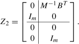
• 1. First, we note that the rank of M ₁ equals 2n and we set a := 2(n + m) − 2n = 2m. Thus, the system contains 2m algebraic variables (the pressure and the part of q, which is not divergence-free). Furthermore, we define $Z_2\in \mathbb {R}^{2(n+m),2m}$ by $Z_2^TM_1 = 0$, i.e.,

  

• 2. As a second step we define $\hat A_2:= Z_2^T N_1 [I_{n+m},\ 0]^T$, which yields

  

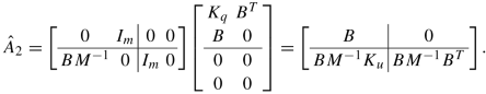
  This matrix has rank 2m, since the full-rank property of B implies that BM ⁻¹ B ^T is invertible. We define d := n − m as the number of differential variables and $T_2\in \mathbb {R}^{n+m,n-m}$ by $\hat A_2T_2 = 0$. Let $C\in \mathbb {R}^{n,n-m}$ be a matrix of full rank with BC = 0 and $C_2 := -(BM^{-1}B^T)^{-1}BM^{-1}K_uC \in \mathbb {R}^{m,n-m}$. Then, we set

  

• 3. Finally, we compute the rank of ET ₂. Since C has full rank, this equals $\operatorname {\mathrm {rank}} MC = n-m = d$. The matrix $Z_1^T := [C^T\ 0] \in \mathbb {R}^{n-m, n+m}$ satisfies

  $$\displaystyle \begin{aligned} \operatorname{\mathrm{rank}} Z_1^T E T_2 = \operatorname{\mathrm{rank}} C^TMC = n-m = d. \end{aligned}$$

Thus, the hypothesis in [39, Hyp. 4.2] is satisfied for μ = 1, which implies that the nonlinear DAE (3.1) has strangeness index one.

Appendix 2: Difference-Algebraic Equation Index of the Considered Systems

In this appendix, we derive the Kronecker index for the discrete schemes considered in Sect. 4.3.

1.1 Half-Explicit Euler

We start with the half-explicit Euler discretisation, that gives a scheme $\mathcal Ex^{k+1} = \mathcal A^k x^k+ h^k$ with the matrix pair

as in (4.4). For sufficiently small τ, due to the definiteness of M and the full-rank property of B, the matrix $\mathcal A$ is invertible and thus, the pair $(\mathcal E, \mathcal A)$ is regular. Let S denote the matrix BM ⁻¹ B ^T. If one applies

from the left and the right, one finds that $(\mathcal E, \mathcal A)$ is similar to

Since B is of full rank, there exists an orthogonal matrix Q and an invertible matrix R such that $BM^{-\frac 12}Q = \big [ 0\ \ R \big ]$ and, in particular,

Thus, the corresponding similarity transformation transforms $(\mathcal E, \mathcal A)$ into

where $\tilde a_{11}$ and $\tilde a_{21}$ stand for unspecified but possibly nonzero block matrix entries. With another few regular row and column transformations, one can eliminate the entry $\tilde a_{21}$ and read off the Kronecker index of ${\bigl ( \mathcal E, \mathcal A \bigr )}$ as the index of nilpotency of which is 2.

1.2 Projection Scheme

The matrix coefficient pair of the Projection scheme (4.9) reads

(6.1)

If we define S := BM ⁻¹ B ^T, if we move the second row and column to the left and bottom, respectively, and if we rescale certain rows and columns, we find that the pair is equivalent to

where the $\tilde e$’s and $\tilde a$’s stand for unspecified but possibly nonzero entries. Since, in particular, S is invertible, one can eliminate the entries $\tilde e_{24}$, $\tilde e_{34}$, $\tilde a_{41}$, and $\tilde a_{14}$ by regular row and column manipulations without affecting the invertibility of the left upper 3 × 3 block in the transformed $\mathcal E$ and read off the Kronecker index of (4.9) as the index of nilpotency of 0 which is 1.

1.3 SIMPLE

The matrix coefficient pair of the SIMPLE scheme (4.13) reads

If we define $S_A := B(\frac 1\tau M^{-1} + A)^{-1} B^T$, move the second row and column to the left and bottom, respectively, and rescale certain rows and columns, then we find that the pair is equivalent to

where, again, the $\tilde e$’s and $\tilde a$’s stand for unspecified but possibly nonzero entries. Since S _A is invertible for sufficiently small τ, we find that this matrix pair has the very same structure as the one of the projection scheme (see section “Projection Scheme” in Appendix) and, thus, is of index 1.

References

Altmann, R., Heiland, J.: Finite element decomposition and minimal extension for flow equations. ESAIM: Math. Model. Numer. Anal. 49(5):1489–1509 (2015)
Altmann, R., Heiland, J.: Regularization and Rothe discretization of semi-explicit operator DAEs. Int. J. Numer. Anal. Model. 15(3), 452–477 (2018)
Arnold, M., Strehmel, K., Weiner, R.: Half-explicit Runge-Kutta methods for semi-explicit differential-algebraic equations of index 1. Numer. Math. 64(1), 409–431 (1993)
Behr, M., Benner, P., Heiland, J.: Example setups of Navier-Stokes equations with control and observation: spatial discretization and representation via linear-quadratic matrix coefficients. Technical Report (2017). arXiv:1707.08711
Benner, P., Heiland, J.: LQG-balanced truncation low-order controller for stabilization of laminar flows. In: King, R. (ed.) Active Flow and Combustion Control 2014, pp. 365–379. Springer, Berlin (2015)
Benner, P., Heiland, J.: Time-dependent Dirichlet conditions in finite element discretizations. ScienceOpen Research, 1–18 (2015)
Braack, M., Mucha, P.B.: Directional do-nothing condition for the Navier-Stokes equations. J. Comput. Math. 32(5), 507–521 (2014)
Brasey, V., Hairer, E.: Half-explicit Runge–Kutta methods for differential-algebraic systems of index 2. SIAM J. Numer. Anal. 30(2), 538–552 (1993)
Brezzi, F., Fortin, M.: Mixed and Hybrid Finite Element Methods. Springer, New York (1991)
Campbell, S.: A general form for solvable linear time varying singular systems of differential equations. SIAM J. Math. Anal. 18(4), 1101–1115 (1987)
Chorin, A.J.: Numerical solution of the Navier-Stokes equations. Math. Comput. 22, 745–762 (1968)
Chorin, A.J., Marsden, J.E.: A Mathematical Introduction to Fluid Mechanics, 3rd edn. Springer, New York (1993)
Ciarlet, P.G.: The Finite Element Method for Elliptic Problems. North-Holland, Amsterdam (1978)
Dai, L.: Singular Control Systems. Lecture Notes in Control and Information Sciences, vol. 118. Springer, Berlin (1989)
Elman, H.C., Silvester, D.J., Wathen, A.J.: Finite Elements and Fast Iterative Solvers: With Applications in Incompressible Fluid Dynamics. Oxford University Press, Oxford (2005)
Emmrich, E., Mehrmann, V.: Operator differential-algebraic equations arising in fluid dynamics. Comp. Methods Appl. Math. 13(4), 443–470 (2013)
Feireisl, E., Karper, T.G., Pokorný, M.: Mathematical Theory of Compressible Viscous Fluids. Analysis and Numerics. Birkhäuser/Springer, Basel (2016)
Ferziger, J.H., Perić, M.: Computational Methods for Fluid Dynamics, 3rd edn. Springer, Berlin (2002)
Fujita, H., Kato, T.: On the Navier-Stokes initial value problem. I. Arch. Ration. Mech. Anal. 16, 269–315 (1964)
Gaul, A.: Krypy – a Python toolbox of iterative solvers for linear systems, commit: 36e40e1d (2017). https://github.com/andrenarchy/krypy
Girault, V., Raviart, P.-A.: Finite Element Methods for Navier–Stokes Equations. Theory and Algorithms. Springer, Berlin (1986)
Glowinski, R.: Finite element methods for incompressible viscous flow. In: Numerical Methods for Fluids (Part 3). Handbook of Numerical Analysis, vol. 9, pp. 3–1176. Elsevier, Burlington (2003)
Gresho, P.M.: On the theory of semi-implicit projection methods for viscous incompressible flow and its implementation via a finite element method that also introduces a nearly consistent mass matrix. I: Theory. Int. J. Numer. Methods Fluids 11(5), 587–620 (1990)
Gresho, P.M., Sani, R.L.: Incompressible Flow and the Finite Element Method. Vol. 2: Isothermal Laminar Flow. Wiley, Chichester (2000)
Griebel, M., Dornseifer, T., Neunhoeffer, T.: Numerical Simulation in Fluid Dynamics. A Practical Introduction. SIAM, Philadelphia (1997)
Ha, P.: Analysis and numerical solutions of delay differential algebraic equations. Ph.D. thesis, Technische Universität Berlin (2015)
Hairer, E., Wanner, G.: Solving Ordinary Differential Equations II: Stiff and Differential-Algebraic Problems, 2nd edn. Springer, Berlin (1996)
Hairer, E., Lubich, C., Roche, M.: The numerical solution of differential-algebraic systems by Runge-Kutta methods. Springer, Berlin (1989)
Hairer, E., Lubich, C., Wanner, G.: Geometric Numerical Integration. Structure-Preserving Algorithms for Ordinary Differential Equations, 2nd edn. Springer Series in Computational Mathematics. Springer, Berlin (2006)
He, X., Vuik, C.: Comparison of some preconditioners for the incompressible Navier-Stokes equations. Numer Math. Theory Methods Appl 9(2), 239–261 (2016)
Heiland, J.: Decoupling and optimization of differential-algebraic equations with application in flow control. Ph.D. thesis, TU Berlin (2014). http://opus4.kobv.de/opus4-tuberlin/frontdoor/index/index/docId/5243
Heinrich, J.C., Vionnet, C.A.: The penalty method for the Navier-Stokes equations. Arch. Comput. Method E 2, 51–65 (1995)
Heywood, J.G., Rannacher, R.: Finite-element approximation of the nonstationary Navier–Stokes problem. IV: Error analysis for second-order time discretization. SIAM J. Numer. Anal. 27(2), 353–384 (1990)
Hinze, M.: Optimal and instantaneous control of the instationary Navier-Stokes equations. Habilitationsschrift, Institut für Mathematik, Technische Universität Berlin (2000)
Karniadakis, G., Beskok, A., Narayan, A.: Microflows and Nanoflows. Fundamentals and Simulation. Springer, New York (2005)
Kunkel, P., Mehrmann, V.: Canonical forms for linear differential-algebraic equations with variable coefficients. J. Comput. Appl. Math. 56(3), 225–251 (1994)
Kunkel, P., Mehrmann, V.: Analysis of over- and underdetermined nonlinear differential-algebraic systems with application to nonlinear control problems. Math. Control Signals Syst. 14(3), 233–256 (2001)
Kunkel, P., Mehrmann, V.: Index reduction for differential-algebraic equations by minimal extension. Z. Angew. Math. Mech. 84(9), 579–597 (2004)
Kunkel, P., Mehrmann, V.: Differential-Algebraic Equations. Analysis and Numerical Solution. European Mathematical Society Publishing House, Zürich (2006)
Ladyzhenskaya, O.A.: The Mathematical Theory of Viscous Incompressible Flow. Gordon and Breach Science Publishers, New York (1969)
Landau, L.D., Lifshits, E.M.: Fluid Mechanics. Course of Theoretical Physics, vol. 6, 2nd edn. Elsevier, Amsterdam (1987). Transl. from the Russian by J. B. Sykes and W. H. Reid.
Layton, W.: Introduction to the Numerical Analysis of Incompressible Viscous Flows. SIAM, Philadelphia (2008)
Leray, J.: étude de diverses équations intégrales non linéaires et de quelques problèmes que pose l’hydrodynamique. J. Math. Pures Appl. 12, 1–82 (1933)
LeVeque, R.J.: Numerical Methods for Conservation Laws, 2nd edn. Birkhäuser, Basel (1992)
Logg, A., Ølgaard, K.B., Rognes, M.E., Wells, G.N.: FFC: the FEniCS form compiler. In: Automated Solution of Differential Equations by the Finite Element Method, pp. 227–238. Springer, Berlin (2012)
Mattsson, S.E., Söderlind, G.: Index reduction in differential-algebraic equations using dummy derivatives. SIAM J. Sci. Comput. 14(3), 677–692 (1993)
Noack, B.R., Afanasiev, K., Morzyński, M., Tadmor, G., Thiele, F.: A hierarchy of low-dimensional models for the transient and post-transient cylinder wake. J. Fluid Mech. 497, 335–363 (2003)
Nguyen, P.A., Raymond, J.-P.: Boundary stabilization of the Navier–Stokes equations in the case of mixed boundary conditions. SIAM J. Control. Optim. 53(5), 3006–3039 (2015)
Pironneau, O.: Finite Element Methods for Fluids. Wiley/Masson, Chichester/Paris (1989) Translated from the French
Raymond, J.-P.: Feedback stabilization of a fluid-structure model. SIAM J. Cont. Optim. 48(8), 5398–5443 (2010)
Reis, T.: Systems Theoretic Aspects of PDAEs and Applications to Electrical Circuits. Shaker, Aachen (2006)
Reynolds, O.: Papers on Mechanical und Physical Subjects. Volume III. The Sub-mechanics of the Universe. Cambridge University Press, Cambridge (1903)
Roubí\({\check {\text c}}\)ek, T.: Nonlinear Partial Differential Equations with Applications. Birkhäuser, Basel (2005)
Saint-Raymond, L.: Hydrodynamic Limits of the Boltzmann Equation. Springer, Berlin (2009)
Shen, J.: On error estimates of the penalty method for unsteady Navier-Stokes equations. SIAM J. Numer. Anal. 32(2), 386–403 (1995)
Steinbrecher, A.: Numerical Solution of Quasi-Linear Differential-Algebraic Equations and Industrial Simulation of Multibody Systems. Ph.D. thesis, Technische Universität Berlin (2006)
Tartar, L.: An Introduction to Navier–Stokes Equation and Oceanography. Springer, New York (2006)
Temam, R.: Navier–Stokes Equations. Theory and Numerical Analysis. North-Holland, Amsterdam (1977)
Taylor, C., Hood, P.: A numerical solution of the Navier-Stokes equations using the finite element technique. Int. J. Comput. Fluids 1(1), 73–100 (1973)
Turek, S.: Efficient Solvers for Incompressible Flow Problems. An Algorithmic and Computational Approach. Springer, Berlin (1999)
Weickert, J.: Navier-Stokes equations as a differential-algebraic system. Preprint SFB393/96-08, Technische Universität Chemnitz-Zwickau (1996)
Weickert, J.: Applications of the theory of differential-algebraic equations to partial differential equations of fluid dynamics. Ph.D. thesis, Fakultät für Mathematik, Technische Universität Chemnitz (1997)
Williamson, C.H.K.: Vortex dynamics in the cylinder wake. Annu. Rev. Fluid Mech. 28(1), 477–539 (1996)
Zeidler, E.: Nonlinear Functional Analysis and its Applications. II/A: Linear Monotone Operators. Springer, Berlin (1990)
Author information
Authors and Affiliations
Corresponding author
Editor information
Editors and Affiliations