
Abstract
This chapter is devoted to isotropic incompressible turbulence. The main features of related theories are discussed, along with the recent results: energy spectrum and two-point correlations and related models, closures for non-linear terms in both physical and Fourier space, theories for grid turbulence decay including fractal grid case, non-equilibrium effects, advanced spectral theories and models for kinetic energy cascade and dynamics in physical space.
To caricature, it can be jokingly said that, once one has eliminated all features of a flow that one understands, what remains is turbulence. This sentence (Mathieu and Scott 2000) is even more relevant in Homogeneous Isotropic Turbulence (HIT), in which no interaction with a structuring effect (mean flow, body force, shock-wave, wall ...) may occur. HIT, even if it can be described statistically with a few number of quantities, is really the core of the turbulence problem.
4.1 Observations and Measures in Forced and Freely Decaying Turbulence
4.1.1 How to Generate Isotropic Turbulence?
Isotropic turbulence can be investigated using both experimental and numerical approaches, despite it requires the existence of an unbounded domain from the theoretical point of view.
A quasi-isotropic fully developed turbulent state can be reached in wind tunnels using a grid to promote turbulence (see Fig. 4.1). In such a setup, boundary layers develop along solid walls, but a quasi-isotropic flow is recovered in the core of wind tunnel. The grid wake transforms a part of mean flow kinetic energy into turbulent kinetic energy. After a certain distance downstream the grid, the mean flow is uniform and no more turbulence production mechanism takes place. Therefore, the turbulent fluctuations dynamics is entirely governed by the advection due to the uniform mean flow, the non-linear interactions and the linear viscous effects, leading to a monotonic decay of the turbulent kinetic energy \(\mathcal{K}\).
Several regions are usually identified downstream the grid, which correspond to different dynamical regimes. These decay regimes are discussed in Sect. 4.1.3.

Schematic view of wind tunnel set-up for generating isotropic turbulence
The full-scale spatial development of isotropic turbulence observed in wind tunnels cannot be exactly reproduced in numerical simulations, due to the enormous required computing power. But it is mimicked switching from a spatially evolving flow to a time-developing flow. In this new configuration, periodic boundary conditions are imposed in all space directions, and a pseudo-turbulent initial condition is used. An isotropic time decaying turbulent flow is then obtained. It can be made statistically steady in time inserting an ad hoc forcing term. But it is worth noting that the use of periodic boundary conditions induces spurious couplings at scales of the order of the computational domain size, and that the analysis of large scale dynamics must be carried out with great care.
Spatially-developing and time-evolving flows can be compared thanks to Taylor’s frozen turbulence hypothesis . In 1938, Taylor hypothesized that the turbulent velocity fluctuation \(\varvec{u}(\varvec{x},t)\) measured by a stationary probe can be interpreted as resulting from the advection of a frozen spatial structure by a uniform steady flow with velocity \(\varvec{U}\), yielding
This hypothesis can also be used to find a approximate relation between space and time derivatives. Let us consider consider a new reference frame advected at velocity \(\varvec{U}\). Denoting quantities expressed in this new reference frame by a tilde, one has:
and
If one now assumes that the signal is frozen in the advected frame, i.e. if \(\partial \tilde{\varvec{u}} / \partial t \approx 0\), then the following relation holds
It is important to note that the Taylor hypothesis does not hold in the following cases, at least from the theoretical viewpoint:
-
A single advecting velocity cannot be defined. This is the case in compressible flows, in which hydrodynamic and acoustic perturbations do not have the same speed, and in flows in which the advection speed depends on the scale of the perturbation. This last case is met in some shear flows (e.g. mixing layers, boundary layers).
-
The rate of change in the moving frame cannot be neglected. Let us consider a structure with characteristic size L and characteristic time T. The Taylor hypothesis is valid if
$$\begin{aligned} \frac{L}{U} \ll T. \end{aligned}$$(4.5)Now using the relation \(\sqrt{\mathcal{K}} \approx L/T\), the validity criterion can be recast as
$$\begin{aligned} \sqrt{\mathcal{K}} \ll U, \end{aligned}$$(4.6)showing that the mean flow speed must be large compared with the characteristic turbulent velocity scale.
One of the first experiment of decaying grid-generated turbulence, but perhaps one of the most documented, was carried out by Comte-Bellot and Corrsin (1966). In order to achieve a better isotropy, at least measured looking at the Reynolds stress tensor, a convergent duct was placed after the grid, in the “formation region”. Without this additional device, the Reynolds stresses exhibit a mild axisymmetry with \(\overline{u^2_1} > \overline{u^2_2} \sim \overline{u^3_2}\): the effect of the convergent duct is to diminish the Reynolds stress component in the axial direction (\(x_1\) here) and to increase it in the radial directions, as shown by Rapid Distortion Theory (see Chap. 8). Unfortunately, such experiments cannot reproduce high Reynolds number flows, a typical value of the Reynolds number based on the Taylor microscale \(Re_{\lambda } = \lambda u'/\nu \) being 70–80. Here \(u' = \sqrt{\frac{2}{3} \mathcal{K}}\) denotes the characteristic velocity scale of the large, energy-containing scales, and \(\lambda \equiv \sqrt{15 \nu u'^2 / \varepsilon }\) is the Taylor microscale,Footnote 1 where \(\varepsilon \) is the kinetic-energy dissipation rate (see Sect. 4.2.1 for more details).
DNS began to reach higher Reynolds numbers from the early 1980s. A weakness of these simulations is that the large scale forcing which is present in the simulation prevent recovering reliable information about the smallest wavenumbers. The semi-empirical law
was recently proposed, where N is the number of grid points along the side of a cubic box in a conventional pseudo-spectral DNS. Using such a high-accuracy method, the recommended mesh size is \(\Delta x \sim 4-5 \eta \), where \(\eta \) refers to the Kolmogorov length scale. This estimate was further refined in the case of freely decaying turbulence by Meldi and Sagaut (2017). To avoid spurious confinement effects, the domain size should be at least ten times larger than the integral scale at the final time of simulation. Therefore, in order to simulate turbulence decay from time \(t_0\) to \(t_F\) with an initial turbulent Reynolds number \(Re_L (0)\), one should take
where \(\sigma \) is the slope of the energy spectrum at very large scales, i.e. \(E(kL \ll 1) \propto k^{\sigma }\).
4.1.2 Main Observed Statistical Features of Developed Isotropic Turbulence
The main results retrieved from laboratory experiments and numerical simulations are the following:
-
Typical observed turbulent kinetic energy spectrum shapes are displayed in Fig. 4.7. An universal inertial range is observed in the turbulent kinetic energy spectrum if the Reynolds number is high enough. At very high wave numbers, viscous dissipation becomes dominant, and the energy spectrum falls very quickly. The physical assumption that the turbulent field is regular in the sense that the \(L_2\) norm of all high order spatial derivatives of the velocity field is finite suggests that the spectrum shape should exhibit an exponential decay at very high wave numbers.
The spectrum shape at large scales (i.e. small wave numbers) which do not belong to the inertial range is observed to be flow-dependent.
The time evolution of the turbulent kinetic energy spectrum is displayed in Figs. 4.7 and 4.8. Results dealing with both the free decay case and the statistically steady case are presented. In the former case, no source of turbulent kinetic energy is present, and the turbulent kinetic energy is a monotonically decaying function of time, while in the latter a kinetic energy source is used to reach a statistically steady state. In both cases, it is observed that the spectrum shape relaxes towards a universal shape at small scales (provided that the Reynolds number is high enough to allow for the existence of the inertial range). The change in the kinetic energy spectrum shape is due to non-linear interactions between modes. Two mechanisms are obviously at play: a direct kinetic energy cascade from large to small scales (also referred to a the forward cascade) which is responsible for the existence of the inertial range, and an inverse kinetic energy cascade from small to large scales (also named the backward cascade) which yield the growth of the energy spectrum at very small wave numbers.
-
Turbulent velocity fluctuations are not Gaussian random variables.
A first manifestation of non-Gaussianity of the turbulent velocity field is that its odd-order statistical moments are not zero, while they are identically zero for a random Gaussian field. A measure of this difference is therefore gained looking at the skewness and the flatness parametersFootnote 2 based on velocity increments (or equivalently the velocity gradients). Common reported values of the skewness factor are \(S_0 = -0.4 \pm 0.1\) (instead of \(S_0 = 0\) for a Gaussian field), while the flatness factor, \(F_0\), ranges from 4 to 40, depending on the Reynolds number (instead of \(F_0 = 3\) for a Gaussian field).
It is worth noting that the single point even moments of velocity fluctuations exhibit a quasi-normal distribution (see Fig. 4.2), while velocity increments are not Gaussian random variables. Therefore, the one-point analysis of the turbulent velocity field is not sufficient to analyze the lack of Gaussianity of turbulence: two-point quantities must be considered. Extreme velocity events, which correspond to the very end of the tails of the pdf plots are observed to escape the Normal distribution. As a matter of fact, the tails of the velocity-increment pdf are observed to be exponential or even stretched exponential. The negative value of the skewness factor is associated to a strong asymmetry in the distribution of longitudinal velocity increment with dominating compressive events. A possible explanation is that this extreme events are (at least partially) governed by the physical mechanisms responsible for the production of turbulent kinetic energy.Footnote 3 Therefore, they are flow-dependent and do not exhibit an universal behavior, since they are sensitive to the characteristic time scale of the turbulence production at large scales.
The analysis of the pdf of the longitudinal velocity increments shows that the lack of Gaussianity is scale-dependent (see Fig. 4.3), in the sense that velocity increments at small scales exhibit larger differences with the Normal distribution than velocity increments at larger scales.
The lack of Gaussianity is an intrinsic feature of turbulence, due to the nonlinearity of the Navier–Stokes equations. This point will be addressed in Sect. 4.11.5.

From Noullez et al. (1997) with permission of CUP
Probability density function of normalized velocity fluctuation in isotropic turbulence.

From Noullez et al. (1997) with permission of CUP
Probability density function of normalized velocity increment in isotropic turbulence.
4.1.3 Energy Decay Regimes
The turbulent kinetic energy \(\mathcal{K}\) is observed to follow different regimes, depending on the position in the wake of the turbulence-generating grid. Three regions are usually identified, which are presented below. They have an universal character, since they are observed in almost all clean experimental data sets.
-
(i)
The formation region, in which the wakes of the rods of the grid interact and merge. These interactions lead to a loss of memory of turbulent fluctuations and to the rise of an quasi-isotropic state.Footnote 4 It is important noting that this return to isotropy is not observed if the initial Reynolds number is too low.
-
(ii)
The initial region, in which the flow can be considered as isotropic and is strongly energetic. In this region, the Taylor-scale-based Reynolds number \(Re_\lambda \) is high, meaning that the non-linear effects are dominant. Both experimental data and theoretical analysis lead to \(Re_\lambda \ge 100\) as a minimum to recover the high-Reynolds decay exponent, higher values being required when higher-order statistics are considered. In this region, the turbulent kinetic energy \(\mathcal{K}\) is observed to decay approximately like \(t^{-n}\) with \(n \approx 1.1{-}1.38\), while the Taylor scale grows like \(t^{0.35-0.4}\). Most existing turbulence theories yield \( 6/5 \le n \le 4/3\), but some significant differences with experimental data are reported. It is important to notice that experimental uncertainties dealing with the measure of the decay exponent are high, since this measure relies on several strong assumptions (Mohamed and Larue 1990; Skrbek and Stalp 2000). This is illustrated in Fig. 4.4 in which the histogram of about 600 values of the decay exponent of kinetic energy in grid turbulence published over the last 50 years is displayed.
Theoretical analyses based on two-point closures, like EDQNM (see Sect. 4.8.6) reveal that the decay exponent n is sensitive to many parameters related to the initial condition, such as the shape of the turbulent kinetic energy spectrum at very small wave numbers at initial time, but also to possible saturation effects due to the finite size of both experimental facilities and computational domains (Skrbek and Stalp 2000). The analysis of these states is presented in Sect. 4.4.
-
(iii)
The final region, which is defined as the region in which the Taylor-based Reynolds number is so low that the viscous linear effects are dominant. The criterion \(Re_\lambda \le 1\) is sometimes used to define the final region, but EDQNM analysis show that \(Re_\lambda \le 0.1\) is a better threshold to observe the asymptotic low-Reynolds behavior. The turbulent kinetic energy now decays more fastly, leading to \(\mathcal{K}\sim t^{-n}\) with \(n \approx 2-2.5\), while the Taylor microscale grows like \(\sqrt{t}\). It is important to note that, at such low Reynolds number, isotropy is very difficult to achieve, either in laboratory experiment and in numerical simulations, due to couplings between large and small scales. As in the previous case, the decay rate is expected to be sensitive to the slope of the spectrum at very low wave numbers and various parameters of the experimental apparatus. Experimental realizations of the final region are very rare, and it seems that the transition between the initial and the final region has never been observed experimentally, since it would require very long wind tunnels (Skrbek and Stalp 2000). Details about this decay regime are displayed in Sect. 4.4.5.

From Meldi and Sagaut (2012) with permission of CUP
Histogram of about 600 published values of the power law exponent \(n_{u^2}\) related to the decay turbulent kinetic energy in DNS and wind tunnel experiments. Grey areas are related to the probabilistic regions predicted by Meldi et al. (2011) for Saffman and Batchelor turbulence using uncertainty quantification techniques to account for possible changes in the initial spectrum.
4.1.4 Coherent Structures in Isotropic Turbulence
Statistical isotropy does not imply that isotropic turbulence fluctuations are uncoherent. Since the pioneering simulations of Siggia (1981), it has been observed that vortical coherent events are present in isotropic turbulence. One usually distinguishes elongated vortices, referred to as worms or vortex tubes, and flat vortex sheets. These structures, their dynamics and their role in the turbulence dynamics are discussed in Sect. 4.10.
4.2 Classical Statistical Analysis: Energy Cascade, Local Isotropy, Usual Characteristic Scales
4.2.1 Double Correlations and Typical Scales
Isotropy implies that the two-point second order correlation tensor
(time is omitted for the sake of brevity) can be expressed as \(R_{ij} = A(r)\delta _{ij} + B(r) r_i r_j\), or
introducing the scaling factor \(u'^2= \frac{2}{3}\mathcal{K}\), and using the longitudinal correlation function
and its transverse counterpart
in which \(\varvec{n}\) is a unit vector normal to \(\varvec{r}\) (see Fig. 4.5).

Schematic view of multi-point correlations. Top: general sketch of the correlation between two-velocity components taken at two differents points A and B. Bottom: illustration of the physical meaning of the longitudinal correlation function f(r) and its transverse counterpart g(r)
The scalar correlation functions f and g are linked via the incompressibility constraint. Using \(\frac{\partial R_{ij}}{\partial r_j}=0\) one obtains
It can be easily seen that
along with
where the notation \(f'\) is introduced to denote the derivative of \(\partial f/ \partial r\) for the sake of simplicity. Finally, reintroducing the time dependency, the evolution equation for the two-point second order tensor amounts to the single scalar equation, e.g. for f, as follows
which is referred to as the Karman–Howarth equation . The term \(R_{LL,L}\) represents the longitudinal two-point third-order correlation function, which is involved via the quadratic non linearity. It is defined as
A slightly different form can be found in Mathieu and Scott (2000).
Typical length scales of turbulence can be defined using functions f(r) and g(r). The longitudinal and transverse integral lengthscales, denoted \(L_f\) and \(L_g\), respectively, are defined as
Isotropy implies
showing that there is only one independent integral scale. These scales are usually interpreted as the typical scale of the most energetic eddies in the flow. The integral scale \(L_f\) is commonly replaced by the characteristic large scale \(L_u = \mathcal{K}^{3/2}/\varepsilon \) that can be easily computed using the outputs of most existing statistical turbulence models developed for engineering purposes within the Reynolds Averaged Numerical Simulation (RANS) framework. It is important noting that \(L_f\) and \(L_u\) are not equal, since
EDQNM results show that the approximation \(L_u \sim L_f\) holds for \(Re_\lambda \ge 100\), while at lower Reynolds numbers finite Reynolds effects become significant.
The longitudinal and transverse Taylor microscales , \(\lambda _f\) and \(\lambda _g\), are computed as
respectively, with
in isotropic flows. This scale is defined as the point at which the osculatory parabola of f(r) at point \(r=0\) defined by \(y(r) = f(0) + f'(0)r +f^{\prime \prime } (0)\frac{r^2}{2} = 1 + f^{\prime \prime } (0)\frac{r^2}{2}\) vanishes. Reminding that
one has
Combining this results with the isotropic relation
one recovers the usual expression for the dissipation rate
Consequently, the Taylor microscales are commonly interpreted as the typical size of eddies at which the maximum of dissipation occurs.
The fourth-order derivative of f at \(r=0\) can be evaluated by the use of the same procedure:
where G is the palinstrophy coefficient defined in Eq. (4.47).
A last family of scales was introduced by Kolmogorov in 1941. Assuming local isotropy, he made the hypothesis that two-point two-time statistical moments of the fluctuating field may be evaluated thanks to dimensional analysis using r, the separation distance, \(\tau \), the time delay, \(\nu \), the fluid viscosity and \(\varepsilon \). Here the physical meaning of \(\varepsilon \) deserves a brief discussion. On can define at least three typical rates looking at time evolution of kinetic energy \(\mathcal{K}\) in isotropic turbulence. The first one is the production rate, \(\varepsilon _P\), associated to production of kinetic energy by a source term, if any. The second one, \(\varepsilon _T\), is associated to the non-linear transfer of kinetic energy toward small scales by the energy cascade mechanisms. It is assumed to be scale-independent within Kolmogorov inertial range in most theories. The last rate is the dissipation rate, \(\varepsilon \), which is related to transformation of kinetic energy into heat via viscous mechanisms. In the case of local equilibrium, one has \(\varepsilon _P = \varepsilon _T = \varepsilon \) and \(\varepsilon \) can be understood as a non-linear energy transfer rate across scales rather than a viscous phenomenon rate.
Several quantities can be build using \(\varepsilon \) and \(\nu \) thanks to dimensional analysis. The Kolmogorov length scale, \(\eta \), time scale \(\tau _\eta \) and velocity scale \(u_\eta \) are given by
The physical meaning of Kolmogorov scales is obtained observing that the local Reynolds number \(Re_\eta = u_\eta \eta /\nu \) =1. Such a low value shows that eddies with size of the order of \(\eta \) are governed by linear diffusive effects. As a consequence, the Kolmogorov scale is commonly accepted as the smallest active scale in a turbulent flow.
Integral, Taylor and Kolmogorov scales whose definitions are summarized in Table 4.1 are tied by scaling laws summarized in Tables 4.2 (for spatial scales) and 4.3 (for time scales).
4.2.2 (Very Brief) Reminder About Kolmogorov Legacy, Structure Functions, ‘Modern’ Scaling Approach
Structure functions are interesting alternatives to velocity correlations at two points, using equivalent \(\varvec{r}\) (two-point) separation vectors, but velocity increments \(\delta \varvec{u}'=\varvec{u}'(\varvec{x}+ \varvec{r}) - \varvec{u}'(\varvec{x})\) instead of \(\varvec{u}' (\varvec{x})\) or \(\varvec{u}'(\varvec{x}+ \varvec{r})\). The structure function of order n is defined as
Now restricting the analysis to the longitudinal structure functions in isotropic turbulence, this expression simplifies as
The counterpart of the longitudinal correlation f is the (longitudinal) second-order structure function \(S_2 (r)\). In homogeneous turbulence, the second-order longitudinal structure function, for instance, is given by
More generally, on can keep in mind that structure functions give information on two-point statistics for \(\varvec{r}\ne 0\), and tend to zero with vanishing \(\varvec{r}\).
The Karman–Howarth equation can be rewritten to obtain an exact evolution equation for \(S_2(r)\). In freely decaying isotropic turbulence, one has:
Kolmogorov originally proposed to scale the structure functions in terms of r and the dissipation rate \(\varepsilon \) only, the first and simplest version (denoted K41, since the seminal paper of Kolmogorov was published in 1941) reducing to
The scaling only results from dimensional analysis, once the physical parameters have been chosen. Of course, this choice relies on nontrivial phenomenological aspects. The scaling holds for an inertial range, i.e. for \(L \gg r \gg \eta \), delineated by a large scale L, comparable to \(L_f\) in Eq. (4.19) and the Kolmogorov scale \(\eta \) given by Eq. (4.29). It is important to notice that the classical Taylor series expansion \(u_i (\varvec{x}+ \varvec{r}) = u_i (\varvec{x}) + \frac{\partial u_i}{\partial r_l} r_l + \cdots \) would yield a different scaling law: \(S_n (r) \sim \left( (\partial u/\partial r) r\right) ^n\). This result, which holds for a smooth, differentiable, velocity field, may be valid for the smallest scales, i.e. \(r < \eta \). The simple fact that the K41 exponent (n / 3) is fractional means that the velocity field is not differentiable in the inertial range, and that self-similar dynamics is expected at such scales.
Modern phenomenological theories continue in search of a more general scaling, replacing the n / 3 exponents by new ones, \(\zeta _n\), called ‘anomalous exponents’, since the former are questioned in the case of internal intermittency . The background argument for introducing such new scaling is to consider a local dissipation rate \(\varepsilon (r)\) which is no longer independent from the size r. The reader is referred to the following books for more details: Monin and Yaglom (1975), Frisch (1995), and Mathieu and Scott (2000).
Finally, let us just mention the famous Kolmogorov’s four-fifths law
which appears as a simplified form of the Karman–Howarth equation (4.33) assuming a steady turbulence (and therefore adding a source term to balance viscous dissipation). It can be further simplified neglecting viscous terms, leading to the popular approximate formula:
Accordingly, the K41 scaling remains unquestioned (at least in HIT at very high Reynolds number) for \(n=3\).
It is important noting that relation (4.36) is an asymptotic scaling law, which requires very high Reynolds numbers to be accurately recovered. In many practical realizations, Finite Reynolds Number effects are present that yield a departure from this relation, as seen from Eq. (4.35). Such departure should not be misinterpreted as intermittency effects.
Introducing the Reynolds-dependent coefficient
one recovers the Kolmogorov law as an asymptotic limit with \(\lim _{Re_\lambda \rightarrow +\infty } C_3 = 4/5\). The convergence is illustrated in Fig. 4.6, in which it is observed that \(Re_\lambda \ge 5.10^4\) is required to recover the 4/5 value in freely decaying turbulence while \(Re_\lambda \ge 5.10^3\) is enough in forced turbulence. A few empirical models that account for the Reynolds-dependency of \(C_3\) and \(S^*_3 (r)\) are displayed in Tables 4.4 and 4.5. Results gathered in this figure follow those of Antonia and Burattini (2006), who proposed one of the best available semi-empirical fit (dotted line) for finite-Reynolds number effects. In addition, EDQNM results are given by solid lines, and the CBC (Comte-Bellot and Corrsin) points were obtained by calculating \(S_3\), using Eq. (4.59), from the spectral transfer terms shown in Fig. 4.21, that are very similar in both experiment and EDQNM calculations.

Courtesy of A. Briard, adapted from an original figure in Tchoufag et al. (2012)
Finite Reynolds Number effects: convergence of \(C_3\) versus the Taylor-based Reynolds number. The Kolmogorov 4/5th-law is recovered when \(C_3 = 4/5\).
4.2.3 Turbulent Kinetic Energy Cascade in Fourier Space
It is often easier to investigate two-point statistics using the three-dimensional Fourier space. The counterpart of Eq. (4.11) in the Fourier space is Eq. (2.134), recalled below
It should be borne in mind that isotropy yields a very special form of the spectral tensor. The involved parameters are the following: E(k, t), with \(k=|\varvec{k}|\), is the usual energy spectrum, representing the distribution of turbulent kinetic energy over different scales and the quantity in brackets will be recognized as the projection matrix, \(P_{ij}(\varvec{k})\). Thus, \(\hat{R}_{ij}\) is determined by a single real scalar quantity, E, which is a function of the sole magnitude of \(\varvec{k}\). Therefore, both the form of \(\hat{R}_{ij}\) at a single point and its distribution over \(\varvec{k}\)-space are strongly constrained by isotropy.
The evolution of the energy spectrum is governed by the Lin equation
in which the third-order correlations are involved in the scalar spectral transfer term T(k, t).Footnote 5 This equation can be seen as a spectral counterpart of the Karman–Howarth equation (4.17). Exact relationship between E(k), T(k) and all the correlations defined in physical space can be found in Mathieu and Scott (2000). This equation derives from the Craya’s equation (2.102) by cancelling mean-gradient terms and by assuming isotropy, so that
Integrating the equation over k yields
and
This allows us to recover the basic equation (4.233), and shows that T(k, t) is a pure redistribution term in the Fourier space. The last relation accounts for the fact that the convection term conserves the total kinetic energy, leading to the well-known result that global kinetic energy is an invariant in inviscid incompressible flows (without boundary conditions).
Typical shapes of E(k), \(2\pi k^2 E(k)\) and T(k) are displayed in Fig. 4.22. It is observed that the peak of the energy spectrum, E(k) is significantly separated from the one of the dissipation spectrum \(2\nu k^2 E(k)\) at large Reynolds number. The transfer term is almost zero in a small zone within the inertial range, negative for smallest k and positive for largest k, the areas of both positive and negative values being exactly balanced. The physical meaning is that small wave number modes lose kinetic energy on the mean due to the non-linear interactions, while large wave number modes gain kinetic energy. The scale located within the inertial range have a zero net transfer. The associated dynamic picture is the celebrated forward energy cascade processFootnote 6: turbulent kinetic energy is injected in the system (by external forcing, hydrodynamic instabilities, ...) at small wave number modes. The energy is then pumped toward higher wave number modes by the non-linear interactions,‘streaming’ in some sense toward modes at which it will be transformed into heat by viscous mechanisms. The inertial range is defined as the zone in which the net transfer is zero. In the inertial zone, the classical Kolmogorov scalingFootnote 7
is observed in both experimental an numerical datasets.
The evolution equation for the dissipation \(\varepsilon \) is recovered from Eq. (4.38) by integrating it over k after multiplication by the factor \(2\nu k^2\), yielding
where the skewness S and the palinstrophy G parameters are defined as
where h is the triple correlation function defined in Eq. (4.18).
This equation is the spectral counterpart of the following evolution equation in the physical space:
Looking at Eq. (4.43), it is clear that the second term in the right-hand-side is negative and corresponds to a viscous destruction mechanism. The first term is essentially positive. A part of T(k) (at large k) is privileged by the \(k^2\) weighting factor, and can be interpreted as a production of \(\varepsilon \) by nonlinear interactions. This point will be further discussed in Sect. 4.11.
The fact that the evolution of \(\varepsilon \) results from the imbalance between two very different terms, whose sum can be efficiently modeled using the purely negative term \(-C_{\varepsilon _2} \frac{\varepsilon ^2}{\mathcal{K}} = -\frac{n}{n+1}\frac{\varepsilon ^2}{\mathcal{K}}\) along with \(\mathcal{K}(t) \propto t^{-n}\) is certainly true in HIT at high Reynolds number, but remains not completely understood. As a matter of fact, the exact equation (4.45) leads to
showing that both \(C_{\varepsilon _2}\) and n should be Reynolds-number and time-dependent in the general case. This point will be further discussed in Sect. 4.6.
We should perhaps say a few words about two-dimensional turbulence. On the one hand, this state corresponds to an extreme anisotropic (axisymmetric) case with respect to three-dimensional HIT, in which two-point correlations are invariant along a direction \(x_{\parallel }\), and with a Dirac distribution of spectral kinetic energy \(e(\varvec{k}) = E(k)/(2\pi k)\delta (k_{\parallel })\). This viewpoint will be addressed in Chap. 7, showing that the accurate description of a partial transition from three-dimensional to two-dimensional structure needs a very refined anisotropic description. On the other hand, one can just get rid of the third dimension and consider HIT in two dimensions as a self-consistent area of study. In this case the scaling
has been proposed by Kraichnan, in connection with the conservation of enstrophy \(\overline{\omega '^2}\) and with an inverse cascade.
4.2.4 Bridging Between Physical and Fourier Space: Some Useful Formulas
It is worth reminding that in isotropic turbulence the Karman–Howarth equation and the Lin equation are equivalent, and that quantities defined in physical space can be expressed using spectral quantities, and vice versa.
A few useful relations are recalled below:
-
(i)
Velocity longitudinal integral length scale:
$$\begin{aligned} L_f \equiv \int _0^{+\infty } f(r) dr =\dfrac{ 3 \pi }{4} \frac{\int _0^{\infty }\dfrac{E(k)}{k} dk}{\int _0^{\infty }E(k) dk} = \frac{1}{2} \int _0^{+\infty } g(r) dr = \frac{1}{2} \int _0^{+\infty } \left[ f(r) +\dfrac{2}{r}f'(r) \right] dr \end{aligned}$$(4.50) -
(ii)
Velocity longitudinal Taylor length scale:
$$\begin{aligned} \lambda _f^2 \equiv - \frac{1}{f^{\prime \prime } (0)} = \dfrac{10 \mathcal {K} \nu }{\varepsilon } = 5 \dfrac{\int _{0}^{\infty } E(k,t)dk}{\int _0^{\infty }k^2E(k,t)dk} \end{aligned}$$(4.51) -
(iii)
Turbulent dissipation rate:
$$\begin{aligned} \varepsilon = \nu \overline{\dfrac{\partial u'_i}{\partial x_j}\dfrac{\partial u'_i}{x_j}}= \nu \overline{\omega '_i \omega '_i} = 2\nu \int _0^{+\infty } k^2 E(k) dk = 10 \frac{\mathcal{K}\nu }{\lambda _f^2} = - 10 f''(0) \mathcal{K}\nu = 15 \nu \overline{\left( \frac{\partial u'}{\partial x} \right) ^2} \end{aligned}$$(4.52) -
(iv)
Longitudinal velocity correlation function as a function of the three-dimensional energy spectrum:
$$\begin{aligned} u'^2 f(r,t) = 2 \int _0 ^{+\infty } E(k,t) \left( \frac{\sin (kr)}{k^3r^3} - \frac{\cos (kr)}{k^2r^2} \right) dk \end{aligned}$$(4.53) -
(v)
Transverse velocity correlation function as a function of the three-dimensional energy spectrum:
$$\begin{aligned} u'^2 g(r,t) = 2 \int _0 ^{+\infty } E(k,t) \left( \frac{\sin (kr)}{kr} - \frac{\sin (kr)}{k^3r^3} + \frac{\cos (kr)}{k^2r^2} \right) dk \end{aligned}$$(4.54) -
(vi)
Three-dimensional energy spectrum as a function of the longitudinal velocity correlation function:
$$\begin{aligned} E(k,t) = \frac{u'^2}{\pi } \int _0 ^{+\infty } kr ( \sin kr - kr \cos kr) f(r,t) dr \end{aligned}$$(4.55) -
(vii)
Spectral energy transfer term (in Lin equation) as a function of the triple correlation function h(r) defined in Karman–Howarth equation by Eq. (4.18):
$$\begin{aligned} T(k,t) = -2 \frac{u'^3}{\pi } \int _0 ^{+\infty } \left[ (k^2r^2 -3) kr \sin (kr) + 3 k^2r^2 \cos (kr) \right] \frac{h(r)}{r} dr \end{aligned}$$(4.56) -
(viii)
Triple correlation function h(r) as a function of the spectral energy transfer term:
$$\begin{aligned} u'^3 h(r) = \int _0 ^{+\infty } \left[ \frac{(k^2r^2 -3) \sin (kr)}{k^4r^4} + \frac{3 \cos (kr)}{k^3r^3} \right] \frac{T(k)}{k} dk \end{aligned}$$(4.57) -
(ix)
Second-order velocity structure function
$$\begin{aligned} S_2 (r) = \overline{ [ u(r) - u(0)]^2} = 2 u'^2 \left[ 1 - f(r) \right] = 4 \int _0 ^{+\infty } E(k) a(kr) dk, \quad a(x)=\frac{1}{3} - \frac{\sin x - x \sin x}{x^3} \end{aligned}$$(4.58) -
(x)
Third-order velocity structure function
$$\begin{aligned} S_3 (r) = \overline{ [ u(r) - u(0)]^3} = - 12 u'^3 h(r) = 4 \int _0 ^{+\infty } \frac{T(k)}{k^2} \frac{\partial a(kr)}{\partial r} dk \end{aligned}$$(4.59)
4.3 Models for Single-Time and Two-Time Energy Spectra and Velocity Correlation Functions
4.3.1 Models for Three-Dimensional Energy Spectrum E (k)
Most existing analytical models for the spectrum E(k) can be recast in the following generic form Pope (2000), Meyers and Meneveau (2008)
where \(f_L\) and \(f_\eta \) are the dimensionless shape functions at large and small scales, respectively. Some consistency relations exist, that lead to integral constraints on the spectrum shape functions:
where \(x = k\eta \) is a dummy variable and \(F(k \eta ) = K_0 f_L( k \eta Re_L ^{3/4} ) f_\eta (k\eta )\). The fluctuating vorticity is defined as \( \varvec{\omega }' = \text {curl} (\varvec{u}')\). The skewness parameter S is given by Eq. (4.46).
The celebrated hypotheses proposed by Kolmorogov in 1941 yield the following asymptotic spectrum shapes for small scales for which the local isotropy hypothesis holds:
where \(K_0\), \(\varepsilon \) and \(\eta \) are the Kolmogorov constant, the dissipation rate and the Kolmogorov scale, respectively.
The assumed regularity of the derivatives of the velocity field is ensured by the function \(f_\eta \), which must be a fastly decaying function, i.e.
Among the numerous proposals made for \(f_\eta (x)\) (see Table 4.7), a widely admitted one is
where C, \(\alpha \), \(\beta \) and n are real parameters. Not to mention values of n such as \(n=4/3\) (proposed by Pao, for pure mathematical convenience), \(n=2\) (suggested by Townsend, assuming linear response of small scales), \(n=1\) is consistently predicted by all “triadic” closures (EDQNM, DIA, LHDIA, LRA) (Kaneda 1993) and supported by recent experimental and DNS results. The reader is referred to Ishihara et al. (2005) for a survey including new DNS with the Taylor micro-scale Reynolds number \(Re_{\lambda }\) and resolution ranging up to about 675 and \(4096^3\), respectively. In addition to \(n=1\), the values of \(\alpha \) and \(\beta \) obtained by the latter DNS decrease monotonically with \(Re_{\lambda }\) and appear to tend to constants as \(Re_{\lambda } \rightarrow \infty \), but the convergence, especially that of \(\beta \), is slow. A simple power law fitting suggests the following asymptotic (infinite \(Re_{\lambda }\)) values
Surprisingly, the above-mentioned closures predict \(\alpha =3\) (Kaneda 1993). This positive value, however, does not yield an overshoot for the spectrum, between the end of the inertial range and the beginning of the dissipative range, because \(\beta \) is sufficiently large.
For small scales much larger than the Kolmogorov scale \(\eta \), one recovers the inertial-range expressionFootnote 8:
The exact value of the Kolmogorov constant is not known. A large number of estimates are provided in the literature (Sreenivasan 1995), coming from measures in the atmospheric boundary layer, from laboratory experiments and numerical simulations. This uncertainty comes from either the departure from isotropy in many flows or the absence of a large inertial range in the spectrum. An reliable estimate seems to be \(K_0 = 1.5 \pm 0.1\).
It is important noting that the Kolmogorov scaling comes from an asymptotic dimensional analysis. Denoting L the integral scale of turbulence, usual estimates for the upper and lower bounds of the inertial range are:
The miminum Reynolds number for an inertial range to exist is an open issue, but there are evidences that the Taylor-scale based Reynolds number \(Re_\lambda \) must be O(100) for any natural inertial range to exist, and that \(Re_\lambda \) = O(1000) for a decade of inertial range.
The shape function at large scale \(f_L\) is purely empirical, since no universal theory exist for such scales. Large scale features are very difficult to measure directly in experiments because of confinement problems and statistical convergence issues. Therefore, they are very often inferred using an a priori model for large scales, whose coefficients are tuned to fit available data. Common sense says that there should be a finite cutoff scale, since real fluid flow always occur in a finite domain (even a very large but finite one like Earth’s atmosphere). In the same way, one should remember that numerical simulations are performed in finite computational domains. As a consequence, one should assume that \(E(k) =0\) for scales larger than a cutoff scale. Such a limit is never taken into account in existing models (see Table 4.6), in which the constraint \(E(k \rightarrow 0) =0\) is enforced.
Several turbulence theories yield to the proposal that E(k) should exhibit an asymptotic algebraic form, i.e.
with \(\sigma \) ranging from 1 to 4. A detailed discussion about the large-scale behavior of the energy spectrum is given in Sect. 4.3.3. Let us just mention here that a detailed analytical analysis show that E(k) might exhibit non-algebraic behaviors in some cases.
4.3.2 Models for Longitudinal Velocity Correlation Function f (r)
The exact form of the function f(r) is unknown. At small separation distance r, the Taylor series expansion of f(r) yields
The asymptotic behavior of f(r) at very large separation distance is still an open issue, and it is often conjectured that \( f(r \rightarrow + \infty ) \sim r^{-m}\) where m is an integer to be determined.
At asymptotically low Reynolds number, i.e. neglecting h(r) in the Karman-Horwarth equation, some analytical solutions can be derived. The most popular one was provided by Taylor in (1935):
Another famous solution is the Gaussian solution provided by Batchelor and Townsend in 1948:
More expression for the asymptotic low-Reynolds case have been proposed (Table 4.7).
At high Reynolds number composite models made of the combination of a Taylor series expansion for \(r \rightarrow 0\) and an algebraic decay law for \(r \rightarrow + \infty \) have been proposed, but almost all of them are not fully satisfactory. The reason for that is that the velocity correlation function must verify a number of physical constraints, and it appears that a model that fulfill all these constraints is still lacking. This is illustrated for a couple low-Reynolds models for f(r) in Table 4.8.
A composite model that fulfill almost all constraints was recently proposed par Monte, Meldi and Sagaut:
where \(f_{in}(r/\lambda , Re_{\lambda })\) and \(f_{out} (r/L, \sigma )\) are related to the behavior at small at large separation distances, respectively. The function \(f_{in}\) is defined as:
where the coefficients \(c_{i}\) are positive functions of \(Re_{\lambda }\). These coefficients have to be tuned in order to take into account the observed \(Re_{\lambda }\) dependency at small r. The outer function is defined as:
where m is the parameter governing the decay dynamics of the two-point velocity correlation. The parameter m is related to the energy spectrum parameter \(\sigma \) thanks to
A least-square optimization procedure based on EDQNM data yields
4.3.3 Remarks on Asymptotic Behaviors \(E(k \rightarrow 0)\) and \(f(r \rightarrow + \infty )\)
Most existing models and theories for the three-dimensional energy spectrum E(k) and velocity correlation function f(r) assume that \(E(k \rightarrow 0) \propto k^{\sigma }\) and \(f(r \rightarrow \infty ) \propto r^{-m}\) where exponents \(1 \le \sigma \le 4\) and \(2 \le m 6\) are tied by a simple univoque relation.
A deeper analysis reveals that this hypothesis stems from an oversimplified mathematical analysis. Starting from the exact relations (4.53) and (4.55) one can show that non-algebraic solutions exists after some rigorous algebra, as shown in Davidson (2011) whose results are summarized in Table 4.9.
The full rigorous solution was given more recently by Llor and Soulard (2013). Considering a correlation function of the form:
they obtained the following exact asymptotic expression:
where \(a_n = (-1)^{n/2} (n-2)/(n-1)!\) (n being restricted to even integers) along with
and
The first term in this expression for E(k) exhibits a logarithmic correction, showing that non-algebraic behavior for E(k) or f(r) must be considered, which has not been the case in almost all existing theories. It is worth noting that these expressions stem from kinematic analysis, and that there is no evidence that they are solutions of the Lin and Karman–Howarth equations.
4.3.4 Model for Wave-number-frequency Energy Spectrum \(E(\varvec{k}, \omega )\)
The energy spectrum models can be extended to obtain a wave-number frequency energy spectrum, which will account for advection of the turbulent scales. Introducing the two-point two-time velocity correlation tensor \( R_{ij} ( \varvec{r}, \tau ) = \overline{u'_i (\varvec{x}, t) u'_j (\varvec{x}+ \varvec{r}, t+ \tau )}\) and its Fourier transform in the physical space
the two-time energy spectrum \(E (\varvec{k}, \tau )\) is defined as
The wave-number-frequency energy spectrum is then obtained applying the Fourier transform in time
To model \(E (\varvec{k}, \omega )\) it is necessary to identify advection mechanisms that are at play, the emphasis being put on small scales for which a universal behavior may be expected. At least three advection mechanisms can be taken into account:
-
(i)
Advection by a mean flow velocity, which will be uniform in the isotropic turbulence case. Small scales are assumed to evolved slowly compared to the mean velocity and to be advected in a quasi-frozen state, as hypothesized by Taylor in 1938 (see Sect. 4.1.1).
-
(ii)
Passive advection by large turbulent scales. This phenomenon was addressed in pioneering works by Kraichnan in 1964 and later by Tennekes in 1975. It is coined as the random sweeping of small scales by large ones.
-
(iii)
Straining by large scale fluctuations, which results in the nonlinear cascade process.
The effects of the first two advection mechanisms can be understood considering an extended version of Kraichnan’s Linear Random Advection model in which both advecting fields are accounted for:
where \(\varvec{u}, \varvec{v}_0\) and \(\varvec{v}\) denotes the small scale velocity field, the mean velocity field and the large-scale velocity field with zero mean, respectively. The exact analytical solution is
which corresponds to Eq. (2.112), with \(G^{(0)}_{ij} (\varvec{k}, t, t_0) = \exp \left[ \varvec{k}\cdot (\varvec{v}_0 + \varvec{v}) t \right] \) and a zero source term \(\varvec{s}\). Here, since the mean flow velocity is assumed to be uniform, one has \(\varvec{k}(t) = \varvec{k}(t_0)\).
The two-time spectral energy tensor is therefore given by
Noting \(\varvec{x}' = \varvec{x}+ \varvec{r}\) and \(t' = t + \tau \) and reminding that
one obtains
Now inserting the solution (4.86), one obtains
which can be rewritten as a relation between two-time and single-time spectral tensors:
Integration over \(\varvec{k}'\) leads to
from which one recovers the relation between two-time and single-time energy spectra:
This expression can be further developed assuming that the sweeping velocity field \(\varvec{v}\) is a Gaussian random field. In this case, one has
showing that the two-time energy spectrum originates in a combination of harmonic oscillations induced by the mean field advection and exponential decay due to random sweeping. The single-time energy spectrum \(E (\varvec{k})\) is not modified and is still fully general at this point. One can note that (4.93) is the Fourier transform of a Gaussian distribution with mean velocity \(\varvec{v}_0\) and a variance specified by the sweeping velocity \(V = \sqrt{ \overline{\varvec{v}^2} /3}\).
Therefore, the associated expression wave-number-frequency spectrum spectrum is Wylczek and Narita (2012)
showing that the mean flow advection induces a Doppler shift in frequency, while random sweeping generates a Doppler broadening of the spectrum in the frequency domain. This model might be further complexified accounting for the Doppler shift induced by the random field \(\varvec{v}\). The energy spectrum \(E (\varvec{k}, \omega )\) may be anisotropic even in the case of an isotropic E(k) because of the Doppler shift term \(\varvec{k}\cdot \varvec{v}_0\).
It is important to note that this model is based on the simplified linear propagator (4.85) which does not account for viscous, pressure and nonlinear effects, allowing for a simple analytical integration. This model is observed to be in satisfactory agreement with DNS data.
A last comment is that these results, including the exponential term due to random sweeping, are recovered considering Taylor series expansions about the isotropic solution (Kaneda 1993; Kaneda et al. 1999). In these references, two-time correlations are obtained computing the coefficient of the time expansion thanks to spectral closures, namely the Lagrangian Renormalized Approximation, which also assumes some degree of Gaussianity for velocity fluctuations.
4.3.5 Models Two-Point Two-Time Velocity Correlation \(R(r, \tau )\)
The longitudinal two-point two-time correlation function \(R(r, \tau ) = R_{11} (r \varvec{e}_x, \tau )\) is classically approximated via polynomial expansion, which aims at expressing it in terms of the single-time correlation function.
Considering advection by a uniform mean flow with a component \(u_0\) along the x-axis, Taylor’s frozen turbulence hypothesis yields the following linear approximation:
which is observed to yield bad results, since iso-correlation contours are straight lines in the (x, t) plane that extend up to infinity, which is unphysical since turbulent eddies have finite correlation scales. A more realistic model is obtained considering higher-order expansions. A second-order Taylor series expansion leads to
Statistical isotropy and stationarity imply
Such an expansion was proposed by Kaneda in a series of papers, e.g. Kaneda (1993), Kaneda et al. (1999), to predict both Lagrangian and Eulerian correlation tensors in isotropic turbulence. In Kaneda et al. (1999) a Padé approximation is used to recover the fact that \(R(r, \tau \rightarrow + \infty ) = 0\), an asymptotic behavior that a simple short-time Taylor series expansion is unable to recover.
A second-order model coined as the Elliptic model or the scale-similarity model is obtained considering an isocontour \(R(r, \tau ) = C\) (He et al. 2009; Zhao and He 2009). This isocontour intercepts the space separation axis at the point \((r_c, 0)\), leading to
Now inserting the second-order expansion (4.96), one obtains
where
leading to the final model
Correlation isocontours are self-similar ellipses, with aspect ratio A and angle with the horizontal axis \(\alpha \) given by the following formula:
The elliptic model is observed to yield very accurate results for small scales within the inertial range, and yields very satisfactory prediction of Taylor and integral scales. Addition of higher-order terms is not observed to yield significant improvement of the results. It is worth noting that the elliptic approximation is not accurate for pressure fluctuations (see Sect. 4.9).
This model accounts for both advection (at velocity \(U_c\)) and random sweeping (with characteristic velocity \(V_c\)) phenomena. It is compatible with the model two-time two-point energy spectrum (4.94), and can be extended to shear flows (see Sect. 9.6.2.1).
As a matter of fact, an exact relation between \(R(r, \tau )\) and the two-time energy spectrum is
Now inserting the model (4.92) and accounting for (4.93), one obtains in the isotropic case (and using notation of the preceding section)
which should also be equal to (using the elliptic model)
A second order expansion yields the following identification
leading to the following identifications: \(U_c = u_0\) and \(V_c = \sqrt{3} V\). The formula above show that the random sweeping by large scales results in an exponential decay of the correlations at small scales, without introducing the viscous damping effect. The elliptic model is reported to be in very satisfactory agreement with DNS data also at relatively large scales for which the truncated Taylor series expansions should not hold. It has not be assessed at very large scales.
The velocities \(U_c\) and \(V_c\) may be measured and evaluated thanks to relations (4.99) and (4.100). They can also be evaluated thanks to dedicated models to recover a predictive model. In the isotropic case, one has
along with
and
where the random sweeping velocity is approximated as \( v^2 =2 \int _0 ^{k_c} E(k) dk\), \(k_c\) the largest wave number associated to large scales. As a first approximation one can take \(v^2 = \mathcal{K}\), leading to
This elliptic model, being coherent with the spectrum model discussed in the preceding section, does not account for viscous, pressure and straining effects. The relative influence of straining and sweeping can be analyzed considering the scale-by-scale evolution of the correlation time.
Defining the two-time correlation coefficient at wavenumber k as
the correlation time at wave number k is defined as \(\tau _D (k) = \int _0 ^\infty C(k,\tau ) d\tau \). Depending on the dominant mechanisms, one should have in the inertial range
Favier et al. (2010) observed in DNS that \(\tau _D (k)\) switch slowly from dominant straining at large scales to dominant sweeping at smaller scales within the inertial range.
4.4 Free Decay Theories: Self-similarity, Self-preservation, Symmetries and Invariants
We now address the issue of free decay of isotropic turbulence, which is assumed to correspond to grid turbulence in wind tunnels. Specific issues related to this flow can be identified, the most popular one being the prediction of decay of the turbulent kinetic energy \(\mathcal{K}(t)\). Tremendous efforts have been devoted to this question since the early 20th century, but a fully satisfactory theory is still lacking. Several related questions have been raised during the past 100 years, among which one must mention:
-
(i)
Does freely decaying isotropic turbulence exhibits self-similar solutions?
-
(ii)
Does kinetic energy follow an algebraic decay law, i.e. \(\mathcal{K}(t) \propto t^{-n}\)?
-
(iii)
Is there a universal decay regime such that \(\mathcal{K}(t) \propto t^{-1}\)?
These questions have been controversial issues during the last decades, and definitive answers are still to be found in many cases.
4.4.1 Self-similarity, Self-preservation and Partial Self-preservation
The very definition of self-similarity, self-preservation or partial self-preservation has been debated during decades, yielding several misunderstanding and controversies. In the present book, the following definitions are selected:
-
(i)
A solution will be said to be exactly self-preserving iff the full solution at any time and any scale can be described using a single length scale \(\ell (t)\) and a single velocity scale v(t), leading to \(\overline{ u'(r,t) u'(0,t)} = v^2 (t) F (r/\ell (t) )\) and \(E(k,t) = v^2(t) \ell (t) G( k\ell (t) )\) where F(x) and G(x) are dimensionless shape functions for the velocity correlation function and energy spectrum, respectively. The very concept of self-preservation (also referred to as the von Karman hypothesis in Monin and Yaglom 1975) was pioneered by Taylor (1935), von Karman and Howarth (1938) and von Karman and Lin (1949).
-
(ii)
A solution will be said to be partially self-preserving if self-preservation is observed over a limited range of scales and not at all scales.
-
(iii)
A solution will be said to be self-similar, according to George’s definition (sometimes referred to as extended self-similarity hypothesis) George (1992), if Lin equation (or equivalently the Karman–Howarth equation) admits a self-similar solution such as \(E(k,t) = E_s(t,\star ) \, \psi (k\ell (t), \star )\), \(T(k,t) = T_s(t,\star ) \, \varphi (k\ell (t),\star )\), where \(E_s\) and \(T_s\) are time-dependent amplitude terms and \(\psi \) and \(\varphi \) shape functions, respectively. Here, \(\star \) denotes a possible dependency on initial conditions. This definition is more flexible than pre-existing self-similarity theory, according to which \(E(k,t) = v^2(t) \ell (t) \, \psi (kl(t),\star )\) and \(T(k,t) = v^3(t) \, \varphi (k\ell (t),\star )\). The difference lies in the fact that no a priori choice is made on both \(E_s\) and \(T_s\) in the former case, while amplitude scalings are fixed in the later.
The self-similarity theories aim at analyzing the statistical structure of the turbulent field, but they also allow for the prediction of the evolution laws of global physical quantities such as kinetic energy \(\mathcal{K}(t)\), turbulent dissipation rate \(\varepsilon (t)\), integral length scale \(L_f(t)\) and Taylor microscale \(\lambda _f (t)\).
The present section is organized as follows. First, symmetry-based analysis of Navier–Stokes equations is discussed in Sect. 4.4.2 along with consequences dealing with the existence of self-similar solutions. The link between symmetry analysis, existence of invariant quantities and algebraic decay of kinetic energy is presented in Sects. 4.4.3 and 4.4.4. Then, the dimensional analysis based Comte-Bellot–Corrsin theory, which bridges between the decay exponent and the features of the initial conditions, is introduced in Sect. 4.4.5. The presentation ends with George’s extended self-similarity theory in Sect. 4.4.6, that starts from the full evolution equations to obtain the two important results: (i) self-similar solutions may exist and (ii) the associated decay exponent depends on features of the initial condition. The results of these theoretical analyses are summarized in Sect. 4.4.7, while the most recent results based on numerical simulations, experimental data and EDQNM analysis are presented in Sect. 4.5
4.4.2 Symmetries of Navier–Stokes Equations and Existence of Self-similar Solutions
Let us first recall that a physical law \(F(x,t; u_1, \ldots , u_N)\) (where x and t denote the space and time, respectively, and \(u_i, i=1, N\) are physical quantities) is said to be invariant under the transformation \( F \longrightarrow F^* , x \longrightarrow x^* , t \longrightarrow t^* , u_i \longrightarrow u_i ^* (i=1,N)\) if and only if
i.e. the physical law is not modified by the change of variables. The Navier–Stokes equations for an incompressible fluid in an unbounded domain (i.e. without boundary conditions) are known to admit the following one-parameter set of symmetriesFootnote 9 (which has the mathematical structure of a Lie group):
-
Time translation:
$$\begin{aligned} (t, \varvec{x}, \varvec{u}, p ) \longrightarrow (t + t_0, \varvec{x}, \varvec{u}, p ) \end{aligned}$$(4.115) -
Pressure translation:
$$\begin{aligned} (t, \varvec{x}, \varvec{u}, p ) \longrightarrow (t , \varvec{x}, \varvec{u}, p + \zeta (t)) \end{aligned}$$(4.116) -
Rotation (with \({{\mathbf {\mathsf{{Q}}}}}\) a constant rotation matrix):
$$\begin{aligned} (t, \varvec{x}, \varvec{u}, p ) \longrightarrow (t , {{\mathbf {\mathsf{{Q}}}}}\varvec{x}, {{\mathbf {\mathsf{{Q}}}}}\varvec{u}, p) \end{aligned}$$(4.117) -
Generalized Galilean transformation:
$$\begin{aligned} (t, \varvec{x}, \varvec{u}, p ) \longrightarrow (t , \varvec{x}+ \varvec{v}(t), \varvec{u}+ {\dot{\varvec{v}}} (t) , p - \rho \varvec{x}\cdot {\ddot{\varvec{v}}} (t)) \end{aligned}$$(4.118) -
Scaling I:
$$\begin{aligned} (t, \varvec{x}, \varvec{u}, p ) \longrightarrow ( \alpha ^2 t , \alpha \varvec{x}, \alpha ^{-1} \varvec{u}, \alpha ^{-2} p) \end{aligned}$$(4.119) -
Scaling II:
$$\begin{aligned} (t, \varvec{x}, \varvec{u}, p, \nu ) \longrightarrow (t , \alpha \varvec{x}, \alpha \varvec{u}, \alpha ^2 p, \alpha ^2 \nu ) \end{aligned}$$(4.120)
where \(\alpha \) is an arbitrary strictly positive real parameter.
It is important noting that these symmetries are identified conducting an exact mathematical analysis of the incompressible Navier–Stokes equations, without introducing any hypothesis or modelling assumptions.Footnote 10
Boundary conditions may eventually decrease the number of symmetries, but cannot introduce new symmetries. It is worth noting that scalings I and II are particular forms (taking \(h= -1\) and \(h=1\)) of the even more general rescaling given below
We now focus on isotropic turbulence. In this case, symmetries such as rotation invariance, Galilean invariance, pressure and time translation are implicitly met. Therefore, the emphasis is to be put on the scaling symmetries and look at the statistical moments of the turbulent velocity field. Let r and f be the correlation distance and the normalized two-point double velocity correlation, respectively (see Sect. 4.2.1 for a detailed description). In the limit of very large Reynolds numbers (i.e. vanishing molecular viscosity), these quantities are transformed as follows (Oberlack 2002)
In the case of finite Reynolds number, the only possible solution is \(\alpha _2 = \alpha _1 ^2\). A set of invariants \(\breve{r}, \breve{f}, \breve{u}, \breve{p}\) can be defined:
where
It is worth noting that, in the finite Reynolds number case, \(\sigma = 1\) is the only possible value. It can be shown, still considering the high Reynolds number limit, that the parameter \(\sigma \) is related to the spatial decay of the two-point correlations and the shape of the kinetic energy spectrum at low wave number:
It is important noticing that the constants involved in these scaling laws are assumed to be independent of time, corresponding to the so-called Permanence of Large Eddies (PLE) hypothesis .
We now show that the existence of self-similar solutions for the isotropic decay problem can be deduced from the symmetry analysis (and not assumed a priori). To this end, let us consider the following one-parameter sub-group of transformation (Clark and Zemach 1998)
where \(\alpha \) is an arbitrary real parameter. This sub-group is labeled by \(\gamma \) and \(t_0\), which are two real parameters. We are now looking for turbulent flows such that the shape of the kinetic energy spectrum E(k, t) is invariant under the transformation (4.129). Simple dimensional analysis yields:
The above property holds for all group elements if it holds for the infinitesimal element, i.e. for the group element \(\alpha = 1 + \delta \alpha \), with \(\delta \alpha \ll 1\). To this end, one differentiates (4.130) with respect to \(\alpha \) and then takes \(\alpha = 1\). The result is the following determining equation:
which can be solved by the method of characteristics in the spectral space. The right-hand side of Eq. (4.131) leads to the following characteristic line equation:
and therefore the wavenumber k evolves as
along the characteristic line spanned by k(0). Along this line, the kinetic energy spectrum evolution is given by the following relation:
leading to the following solution:
Introducing the lengthscale \(\ell (t)\) and the energy scale \(v^{\prime 2} (t)\) such that
one obtains
in which the non-dimensional shape function F is such that
Therefore, the solution obeys a self-similar decay regime.Footnote 11 The important conclusion is that (4.137) is not postulated as in early studies like those of Karman and Howarth in the late 1930’s, but deduced as being a consequence of the symmetries of the governing equations in the limit of very high Reynolds number.
4.4.3 Algebraic Decay Exponents Deduced from Symmetry Analysis
The symmetry analysis introduced in the previous section can also be used to recover some information about the time evolution of the solution. This is done finding the values of \(\sigma \) in Eq. (4.127) or \(\gamma \) in Eq. (4.129).
Time scaling laws for the turbulent kinetic energy \(\mathcal{K}(t)\), turbulent dissipation \(\varepsilon (t)\), integral lengthscale \(L_f(t)\) and turbulent Reynolds number \(Re_L\) are deduced from relation (4.126) in a straightforward way:
It is seen that the time evolution exponents of these global turbulent parameters are explicit functions of \(\sigma \). Since \(\sigma \) is also related to the shape of the kinetic energy spectrum at very large scales (see Eq. (4.128)), this leads to the conclusion that the self-similar decay regime is governed by the very large scales of turbulence.
Different values for \(\sigma \) have been proposed during the past decades, which are now briefly surveyed (corresponding time evolution exponents are displayed in Table 4.10). A value of \(\sigma \) is associated to the existence of an invariant quantity which will remain constant during the decay (see below). In some cases the existence and the physical meaning of this invariant quantity are easily handled, while some controversies exist in other cases. The most popular values for the parameter \(\sigma \) are:
-
\(\sigma = 4\). According to the Loitsyansky-Landau theory, it was hypothesized by Loitsyansky in 1939 that the following integral quantity (referred to as the Loitsyansky integral or the Loitsyansky invariant)
$$\begin{aligned} \mathfrak {I}= - \int r^2 \overline{ \varvec{u}' ( \varvec{x}) \cdot \varvec{u}' ( \varvec{x}+ \varvec{r}) } d ^3\varvec{r}= 8 \pi {u'^2} \int _0 ^{+\infty } r^4 f(r) dr \end{aligned}$$(4.143)is invariant in time during the decay phase. The corresponding time evolution exponents where derived by Kolmogorov in 1941. The associated form the kinetic energy spectrum is referred to as the Batchelor spectrum :
$$\begin{aligned} E(k) = \frac{\mathfrak {I}}{24 \pi ^2} k^4 + \cdots \quad (kL_f \ll 1) \end{aligned}$$(4.144)The time invariance of \(\mathfrak {I}\) is a controversial issue since it depends on the decay rate of velocity two-point correlation at long range. It is constant if velocity long-range interactions decay fast enough, which is not obvious since the pressure fluctuations may induce stronger long-range interactions.Footnote 12 The controversy was initiated by Proudman and Reid in 1954, followed by Batchelor and Proudman in 1956, who advocated that long-range interactions are strong enough to render \(\mathfrak {I}\) time dependent. Since that time, \(\mathfrak {I}\) has been observed to be time-dependent in many numerical simulations, in agreement with predictions of many two-point closures like EDQNM. This issue was very recently revisited by Davidson and coworkers (Davidson 2004; Ishida et al. 2006), who observed that \(\mathfrak {I}\) becomes time independent after a transient phase in high-resolution DNS, provided that the domain size is much larger that the turbulent integral scale (they considered a ratio up to 80) and that the Reynolds number is larger than 100. Therefore, time dependency observed in previous simulations was an artefact due to spurious long-range correlations induced by the insufficient domain size and periodic boundary conditions. The fact that pressure fluctuations do not lead to a strong long-range coupling may be attributed to a screening effect in fully developed turbulence: long-range correlations are weakened by opposite cancelling effects of the very intricate turbulent vorticity field.
-
\(\sigma = 2\). This second value was proposed in 1954 by Birkhoff, who made the hypothesis that the following integral quantity is invariant (referred to as the Birkhoff integral but also as the Saffman integral) :
$$\begin{aligned} \mathfrak {S}= \int \overline{ \varvec{u}' ( \varvec{x}) \cdot \varvec{u}' ( \varvec{x}+ \varvec{r}) } d^3 \varvec{r}= 4 \pi {u'^2} \int _0 ^{+ \infty } r^2 \left( 3 f + r f'(r) \right) dr. \end{aligned}$$(4.145)The corresponding time behavior of the solution was derived by Saffman in 1967, after he argued that the Loitsyansky integral is diverging in isotropic turbulence. For that purpose, Saffman revised the approach introduced by Comte-Bellot and Corrsin in 1966 to investigate the connection between the energy spectrum and the energy decay. The associated spectrum shape (the Saffman spectrum) at large scales is
$$\begin{aligned} E(k) = \frac{\mathfrak {S}}{4 \pi ^2} k^2 ... \quad ( kL _f\ll 1). \end{aligned}$$(4.146) -
\(\sigma =1\). This value was proposed by Oberlack (2002), who emphasizes that this is the only value of \(\sigma \) which allows for the full similarity of the Karman–Howarth equation (see Eq. (4.17) and the corresponding subsection) at finite Reynolds number. A noticeable feature of this solution is that the decay occurs at constant turbulent Reynolds number.
-
\(\sigma = + \infty \). This solution was also proposed by Oberlack in 2002. It corresponds to a decay with constant integral scale.
4.4.4 Time Variation Exponent and Inviscid Global Invariants
The direct physical interpretation of the value of the decay parameter \(\sigma \) is unclear in some cases. It is possible to get a deeper insight into the related physics looking at the links that exist between the choice of a value for \(\sigma \) and the conservation of exact invariants of inviscid flows.
Following Oberlack (2002), let us first recall that, for an inviscid flow in an unbounded domain V, the following non-local conservation laws are exact:
Now using the change of variable based on the invariants introduced in Eq. (4.126), the three conservation laws can be rewritten as follows:
The kinetic energy is strictly positive in a turbulent flow, while the sign and the absolute value of angular momentum and the helicity are not a priori known. Since a choice for \(\sigma \) can enforce only one of the three conservation laws given above, it makes sense to assume that the total linear momentum and helicity are identically null, while the kinetic energy is preserved, yielding \(\sigma =2\). Therefore, the Birkhoff-Saffman theory is coherent with the preservation of kinetic energy at infinite Reynolds number.
Another interpretation is possible (Davidson 2004) since both Loitsyansky and Birkhoff integral quantities are related to exact dynamical invariants of inviscid motion in an unbounded domain. The first one is the linear impulse, \(\mathfrak {I}_{\text {LI}}\), and the second is the angular momentum, \(\mathfrak {I}_{\text {AM}}\), with
Considering a volume V filled by isotropic turbulence with a characteristic length much larger that the integral length scale of the turbulent motion, the following relations hold
If turbulent eddies have a finite, non-negligible linear momentum, then \(\mathfrak {S}\ne 0\) and therefore the spectrum will be of Saffman type and \(\sigma = 2\). If their linear momentum is very small but their angular momentum is finite, then \(\mathfrak {S}\simeq 0\) and \(\mathfrak {I}\ne 0\), yielding a Batchelor-like spectrum and \(\sigma = 4\).
Let us just note that, if the two-point correlations fall sufficiently rapidly to ensure that all integrals are convergent, the following Taylor series expansion holds at small wave numbers:
4.4.5 Comte-Bellot – Corrsin Theory
The theory proposed by G. Comte–Bellot and S. Corrsin for high-Reynolds decay regime relies on dimensional analysis and the following model spectrum
where \([C_\sigma ] = [L]^{\sigma +3}[T]^{-2}\) is a parameter. The Permanence of Large Eddies hypothesis consists in assuming that it is time-independent. The scale L(t) is related to the integral scale and characterizes the energy spectrum peak. This model is an exactly self-preserving solution.
Assuming that the Permanence of Large Eddies hypothesis holds, simple dimensional analysis and spectrum continuity at \(kL=1\) lead to
Turbulent kinetic energy can then be approximated as
from which one obtains the following time-evolution law:
An algebraic decay law that depends on the initial condition via \(\sigma \) is recovered, in accordance with the idea that exact self-preservation leads to algebraic deacy laws. The breakdown of Permanence of Large Eddies hypothesis, i.e. the dependency of \(C_\sigma \) may be taken into account replacing \(\sigma \) in the expressions for the time exponent by \((\sigma -p)\) where the correction factor p is to be determined experimentally of using a more complex model. Results are summarized in Table 4.11.
The theoretical analysis based on the EDQNM closure shows that \(C_\sigma \) is constant in time and \(p = 0\) for \(\sigma \le 3\), while \(p \simeq 0.5\) for \(\sigma = 4\). Therefore, one has \(n = -6/5\) for \(\sigma =2\) and \(n=-1.38\) for \(\sigma =4\). Neglecting the time variation of \(C_4\), one recovers the Kolmogorov value of \(n= -10/7 \simeq -1.43\) for \(\sigma =4\).Footnote 13
Typical numerical results (obtained using simplified numerical models, since these data cannot be obtained by experimental means and are out of range of available supercomputing facilities) are displayed in Fig. 4.7. Turbulent flows with an initial small wave-number slope higher than 4 are observed to relax towards the \(\sigma =4\) solutions at large scales.

From Clark and Zemach (1998) with permission of AIP
Evolution of the kinetic energy spectrum in the initial stage decay. Top: emergence of self-similarity and validation of the PLE hypothesis for \(k^1\) scaling at low wave number. Middle: emergence of self-similarity and validation of the PLE hypothesis for \(k^2\) scaling at low wave number. Bottom: emergence of self-similarity with a \(k^4\) behavior for initial Gaussian-shaped spectrum, and PLE hypothesis breakdown for the \(k^4\) spectrum.
All results displayed above in this section are related to the initial stage of decay, i.e. the asymptotic high-Reynolds regime, which is governed by non linear interactions. They are observed to be very accurate, since the error on the exponents of the different quantities compared with EDQNM simulations is within 1% in all cases for all quantities (Meldi et al. 2011; Meldi and Sagaut 2012, 2013a). The previous analysis can be extended to asymptotically low-Reynolds numbers, i.e. to the final stage of decay. Before doing that, it is worth reminding that neglecting convective terms the exact solution to the Lin equation reads
which is not well suited for quick algebraic manipulation. Assuming that at very low Reynolds number wave number larger than 1 / L have a negligible kinetic energy, one can write
Assuming that dynamics is governed by viscous effects, dimensional analysis leads to \(L(t) = \gamma \sqrt{ \nu t }\), where \(\gamma \) is a dimensionless parameterFootnote 14 and therefore
and
Results are summarized in Table 4.11. They are observed to be as accurate when compared to EDQNM results as in the high-Reynolds number case. Breakdown of PLE hypothesis at very low Reynolds number has never been studied or even reported, therefore no correction is added here to power-law exponents.
Long-time evolution of the kinetic energy spectrum computed with an EDQNM closure is displayed in Fig. 4.8. It is observed that a self-similar final stage of decay is reached at very long time. Here \(\tau \) denotes the eddy turnover time scale associated with the peak of the spectrum at the initial time: \(\tau = ( k^3 _{\text {max}} (0) E ( k_{\text {max}}, 0) ) ^{-1/2}\). It is also noticed that, in the final viscous decay stage, the PLE holds, even in the present case in which \(E(k,0) \sim k^4\) at very large scales.
It is worth noting that \(\sigma = 1\) is related to a singular regime, since decay occurs at constant \(Re_L\) along with \(\mathcal{K}(t) \propto t^{-1}\), for both high-Reynolds and low-Reynolds decay regimes.
An interesting problem is the time needed to reached the final stage of decay starting from a high-Reynolds number solution initially governed by a non linear initial decay stage. The time evolution of the effective time decay exponent n(t) defined as
is displayed in Fig. 4.9 for different values of the spectrum low-wave-number power-law exponent.
It is observed that in all cases a very long time is needed before the solution reach the final stage of decay, i.e. \(n = const.\) The turbulence quickly reaches a cascade-dissipation equilibrium for the \(k^1\) spectrum.Footnote 15 For other spectrum shapes, the transition is too long to be observed (Clark and Zemach 1998). Considering a wind tunnel with air and a mean flow velocity equal to 20 m s\(^{-1}\), a grid-generated turbulence such that \(\mathcal{K}(0) = 20\) m\(^2\) s\(^{-2}\) and the initial turbulent Reynolds number is equal to \(Re_L = 3 000\), the wind tunnel length required to reach the final stage is of the order of \(10^{16}\) m (about one light-year, or about one-third the distance to the nearest star!) for \(k^2\)-shaped spectrum, and \(5.10^6\) m (almost an Earth radius!) for \(k^4\) spectra.

From Clark and Zemach (1998) with permission of AIP
Evolution of the kinetic energy spectrum with transition from the initial stage decay to the final stage of decay.

From Meldi and Sagaut (2013a) with permission of Taylor & Francis
Evolution of the free decay exponents of kinetic energy (top-left), dissipation (top-right), integral velocity scale L (bottom-left) and length scale \(\mathcal{K}^{3/2}/\varepsilon \) versus \(Re_\lambda \) for large-scale spectrum slope \(\sigma =1,2,3,4\). \(\sigma =1\) is discontinuous, since \(Re_\lambda \) is constant in time for that solution.
Previous analyses can be extended to account for more physical phenomena. Skbrek and Stalp introduced a small scale cutoff to account for the very fast damping at scales smaller than the Kolmogorov scale \(\eta \) and a low-wavenumber cutoff to account for possible saturation effects. Saturation occurs if turbulence evolves in a finite-size box. Since L(t) is growing in time in all cases, it will reach the size of the box in a finite time. After that time, L(t) becomes time-independent and no scale larger than L can exist. This can be modeled in a smart and simple way setting \(\sigma = + \infty \) in the high-Reynolds regime formula, yielding \(\mathcal{K}(t) \propto t^{-2}\) after saturation, whatever was \(\sigma \) at initial time. Saturation is therefore associated to a bifurcation in the flow dynamics and a change in the time exponents of all quantities. Both analytical developments and EDQNM simulations show that introducing the small scale cutoff does not change the classical results.
It is important noting that the Comte-Bellot–Corrsin theory is compatible with the symmetry-based analysis discussed in Sect. 4.4.3, i.e. its results encompass those found in previous section. Decay exponents are the same in cases that can be addressed by symmetry analysis, but this theory is also more general since it allows to include more physics (cutoff at small scales, saturation effects, arbitrary values of \(\sigma \)).
One can also identify invariant quantities during the decay using exponents displayed in Table 4.11. Taking \(\mathcal{K}(t)\), L(t) and \(\eta (t)\) as independent variables, one can built two invariants \(I_L (\sigma ) \equiv \mathcal{K}^\alpha L\) and \(I_\eta (\sigma ) \equiv \mathcal{K}^\beta \eta \) where
at high Reynolds number (\(Re_\lambda \ge 200\) in practice). The Saffman invariant and the Loitsyansky’s invariant are recovered as \(I_L(2)\) and \(I_L(4)\), respectively. In the later case, one must observe that the p correction is not taken into account in the original theory, yielding slow drift of that quantity.
In the low-Reynolds number asymptotic regime (\(Re_\lambda \le 0.1-0.01\) in practice), one as
The differences in the expressions of \(\alpha \) and \(\beta \) at low- and high-Reynolds number show that it is impossible to define exact Reynolds-independent quantities that may remain invariant over arbitrary long times, i.e. during the transition between the two regimes. The only case in which such exact invariants may be defined is \(\sigma = 1\), in which \(\alpha = \beta = 1/2\) in both regimes and there is only one independent invariant, which is proportional to the Reynolds number since \(I_L (1) \propto I_\eta (1) \propto Re_\lambda \propto Re_L\). But it is important to note that some “finite-but-long-time” invariant quantities may be encountered as long as the Reynolds number is high enough or once it has reached the low-Re asymptotic regime. In these cases, both \(I_L (\sigma )\) and \(I_\eta (\sigma )\) will be almost constant and can be considered as invariant quantities. It is important to notice that, in these cases, any function depending only on these two quantities will be invariant, showing that an infinite number of invariants can be defined.
4.4.6 Georges’ Extended Self-similarity Theory
George (1992), George and Wang (2000) proposed a theory for the decaying homogeneous isotropic turbulence in which self-preserving solutions of the Lin equation for E(k) are found. The new feature with respect to older self-similarity theories is that both the spectrum and the nonlinear transfer terms are not assumed a priori to scale with a single length and velocity scale.
The starting point is to express the energy spectrum E(k) and the spectral transfer function T(k) under the following the self-preserving forms:
with \( \xi = k\ell \) where \(\ell =\ell (t,\star )\) is a characteristic length scale to be determined. The argument \(\star \) denotes a possible dependence on initial conditions. Differentiating Eq. (4.169) leads to
where the prime denotes the differentiation with respect to \(\xi \). Substituting into the Lin equation and dividing by \( \nu E_s /\ell ^2\) to obtain a dimensionless equation, one obtains
where the dependency on t, \(\xi \) and \(\star \) have been suppressed for the sake of simplicity. Bracketed terms are independent dimensionless parameters. George’s analysis relies on that equation. In practice, self-similar solutions are sought keeping all terms (i.e. considering all physical mechanisms) or neglecting some of them. Observing that the coefficient of the last term is time independent, self-preserving solutions exist iff all other bracketed terms are also time independent.
Keeping all terms in the dimensionless Lin equation (4.171), one get
The second condition straightforwardly leads to
where integration factor was taken equal to 2A for the sake of convenience and \(t_0\) can be eliminated by an adequate choice of time origin. Then, hereafter \(t_0\) will assumed to be zero without loss of generality. Combining the first and the third condition one get
where p is a constant. By integrating one obtains the following power-law decay
The third condition in Eq. (4.172) is satisfied iff
One has
where the integral term is time independent, leading to
Equations (4.173), (4.175) and (4.178) lead to the following algebraic evolution law
then
with \(n=p-1/2\), where p or n must be determined using experimental data or more complex theories.
Now considering the dissipation rate \(\varepsilon \), one obtains
Now recalling that the energy dissipation \(\varepsilon (t)\) in isotropic turbulence reads
and comparing Eq. (4.181), the characteristic length \(\ell \) is observed to scale as the Taylor microscale \(\lambda _f\), i.e.:
Therefore, relation (4.173) yields the following result
showing that \(\lambda _f (t) \propto \sqrt{t}\), in agreement with the Comte-Bellot – Corrsin theory. The coefficient A can be related to the decay law exponent n using the kinetic energy equation
and Eq. (4.182). Thus one obtains
which is the result obtained by von Karman and Howarth (1938). As a consequence the Taylor-based Reynolds number evolves as
The transfer function amplitude \(T_s\) can now be evaluated using \(\lambda \sim \ell \) in a straightforward way:
Among the main conclusions of George’s theory, one can mention that the Lin equation admits self-preserving solutions with the following characteristics
-
The characteristic length scale for the entire spectrum is the Taylor microscale \(\lambda _f\) which evolves as \(\lambda _f \sim t^{1/2}\). As a consequence, the Reynolds number characterizing the turbulent motion is \(Re_\lambda \).
-
The energy follows a an algebraic decay law, i.e. \(\mathcal{K}(t) \propto t^n\), where n is a parameter to be determined.
-
The constant of proportionality and the exponents are fixed by the initial conditions and are flow-dependent.
All these results are coherent with those issued from the Comte-Bellot–Corrsin theory. Introducing additional assumptions makes it possible to obtain new decay regimes. In practice, this is done assuming that one or several bracketed terms in Eq. (4.171) are identically zero. As an example, the famous Kolmogorov “local equilibrium” similarity solution is recovered considering that the two first bracketed terms are zero. A very interesting extension of these results dealing with the possibility of non-algebraic, exponential decay laws for \(\mathcal{K}(t)\) was obtained by George (2000).
Assuming that decay occurs with a time-independent characteristic length, i.e. taking \(d\ell /dt = 0\) and \(\ell =\ell _0\) and setting the second bracketed term equal to zero, integrating the first bracketed term yields
along with
This result is important, since this is the unique case in which a non-algebraic decay law is predicted. George’s extended self-similarity is the only one able to predict such a behavior.
4.4.7 Sum of Results
All theories for isotropic turbulence decay yield coherent results, which can be summarized as follows:
-
(i)
Self-similar solutions might exist and are tied to the existence of invariant quantities. The existence of such solutions is further discussed in Sect. 4.5.2. Arbitrary values of the decay exponent of kinetic energy, i.e. \(\mathcal{K}(t) \sim t^{-n}\) with \( n \ge -1\), may be obtained by arbitrarily neglecting some terms in the equations and prescribing some invariant quantities as found by von Karman and Howarth (1938), or in an equivalent way according to Noether’s theorem, enforcing a symmetry in the problem (Clark and Zemach 1998; Oberlack 2002). As an example, neglecting the nonlinear term yields an approximation for the low-Reynolds final period of decay, while neglecting the viscous term is classically done to analyze the initial high-Reynolds period of decay.
-
(ii)
Kinetic energy exhibits an algebraic decay whose time exponent depends on the initial condition, more precisely on the shape of the spectrum at very large scales. This spectrum shape can also be related to some integral invariant quantities (each spectrum shape is related to specific invariants) or equivalently to some symmetries.
-
(iii)
The Taylor microscale evolves independently of the Reynolds number and the initial condition with \(\lambda _f (t) \propto \sqrt{t}\).
-
(iv)
In the general case, two asymptotic decay regimes are identified, the first one at very high \(Re_\lambda \) and the second one at very low \(Re_\lambda \).
-
(v)
Assuming exact self-preservation and inserting associated expressions for two-point velocity correlation and energy spectrum in Eqs. (4.17) and (4.38), one finds that there is a unique solution when keeping all terms in these two equations: \(\ell (t) = \lambda _f (t) \sim t^{1/2}\) and \(\mathcal{K}(t) \sim t^{-1}\), as recognized since the pioneering works on the subject, e.g. Dryden (1943) and Batchelor (1948).
-
(vi)
The case \(E(k) \propto k\) at very large scales (i.e. \(\sigma =1\)) is a singular case, since decay occurs at constant \(Re_\lambda \) along with \(\mathcal{K}(t) \propto t^{-1}\). In this very unique regime all length scales (integral scale, Taylor scale, Kolmogorov scale) have the same growth exponent 1 / 2.
4.5 Recent Results About Decay Regimes
4.5.1 Power-Law Exponent in the Transitional Decay Regime
Most theoretical predictions of the power-law exponents given in the preceding section originate in asymptotic high- or low-Reynolds developments. This is not explicitly mentioned in the Comte-Bellot–Corrsin analysis, but this is implicitly assumed when chosing the simplified spectrum model for E(k). Therefore, a theory that bridges between the two asymptotic regimes to describe turbulence decay at finite Reynolds numberFootnote 16 would be very useful, since it would correspond to the majority of existing experiments and Direct Numerical Simulations.
A proposal was recently made by Djenidi and Antonia (2015), Djenidi et al. (2015) who developed a theoretical analysis for partially self-preserving decay of isotropic turbulence. Considering the Karman–Howarth equation for the second-order structure function (4.33) equipped with the closure \(S_3 = S S_2^{3/2}\), where S is the skewness given in Eq. (4.46), and performing an analysis similar to George’s one, these authors proved that the decay exponent n of \(\mathcal{K}(t)\) obeys the following relation:
where \(\ell (t)\) denotes the (unique) length scale for which self-preservation is obtained at all scales. It has been seen above that exact self-preservation is obtained in the sole case \(\sigma =1\). Therefore, to extend that result to more realistic cases in which only partial self-preservation exist, the authors propose to take the Taylor scale as a characteristic scale, i.e. \(\ell = \lambda \), leading to the semi-empirical law
This formula is consistent with the Comte-Bellot–Corrsin theory whose results are recovered for both high- and low-Reynolds number regimes.
4.5.2 Do Self-similar Solutions Exist?
The physical relevance of self-similar or self-preserving solutions is a non trivial issue, as emphasized by Batchelor (1953, p. 148): “The assumption of similarity of shape of the statistical functions during decay in the earlier work was principally a mathematical device, used to enable definite results to be obtained ... To find such solutions has been one task; to determine the conditions under which they can and do provide a correct description of turbulence is another. In this latter task which has engaged much attention in the last five years, but even so most of the established results are negative, and our positive results still rest insecurely on vague intuitive arguments (vague for most of us - clear and precise for the inspired few !)”. While exact self-preservation is appealing from a theoretical and mathematical viewpoint, its physical relevance has been questioned very early. As a matter of fact, early experimental results did not support exact self-preservation, while they were in much better agreement with theoretical results based on incomplete self-preservation, leading Hinze to state that (Hinze 1975, p. 162): “Hence it appears to be impossible to take one simple characteristic length for the entire wavenumber range to make the energy spectrum self-similar during decay. It is possible to assume only incomplete self similar preservation ... we may do so for the wavenumber of the energy-containing eddies plus the absolute equilibrium range” and Monin and Yaglom (1975) to qualify it as “definitely incorrect”.
Despite such solutions are the cornerstones of almost all existing theories for isotropic turbulence decay, their existence has been an open issue until the very recent past. The main difficulty is that a direct measurement of the spectrum E(k) at very large scales is almost impossible in both wind tunnel experiments (because of statistical convergence issue and confinement effects) and direct numerical simulations (for grid resolution and computational cost reasons). What is measured in practice is the kinetic energy decay rate, whose relation with the spectrum shape is inverted to recover an estimate for the parameter \(\sigma \). But in such a procedure one makes two key assumptions: i) self-similar solutions exist whose large-scale behavior is \(E(k) \propto k^\sigma \) and ii) only self-similar solutions lead to an algebraic decay law \(\mathcal{K}(t) \propto t^{-n}\) where the decay exponent \(n(\sigma )\) is given by the theories discussed in the preceding section.
It has been shown recently that the both assumptions are wrong the general case and that algebraic decay law can be recovered for non-self-similar solutions.
An exhaustive EDQNM analysis has been carried out by Meldi and Sagaut (2013a), who have shown that in the general case there exist no unique length scale \(\ell (t)\) that allow for a description of the solution using a unique time-independent spectrum shape function. The only exception is the case \(\sigma =1\), which is the only one that exhibits complete self-similarity, in agreement with the fact that all length scales have the same time exponent. The same conclusions hold for the transfer function T(k). Typical results are displayed in Figs. 4.10 and 4.11. It is seen that partial self-preservation is observed on E(k) (based on the integral scale for large scales and Kolmogorov scales for very small scales), while no such behaviour appears on the transfer function T(k).

Rescaled energy spectrum E(k) at different EDQNM simulation times/Reynolds numbers. Scaling is based on (from left to right) integral scale, Taylor scale and Kolmogorov scale. Initial condition was chosen such that \(E(k) \propto k^{\sigma }\) at large scales with \(\sigma = 4\) (top), \(\sigma = 2\) (medium) and \(\sigma = 1\) (bottom)

Rescaled transfer function T(k) at different EDQNM simulation times/Reynolds numbers. Scaling is based on (from left to right) integral scale, Taylor scale and Kolmogorov scale. Initial condition was chosen such that \(E(k) \propto k^{\sigma }\) at large scales with \(\sigma = 4\) (top), \(\sigma = 2\) (medium) and \(\sigma = 1\) (bottom)
4.5.3 Which Scales Govern the Energy Decay Rate?
Another interesting issue in isotropic turbulence decay theory is to identify which scales govern the decay rate, i.e. determine the value of the decay exponent of kinetic energy. In most existing theories (see Sect. 4.4), the decay exponent is expressed as a function of the parameter \(\sigma \), which is usually interpreted as the slope of the energy spectrum at asymptotically large scales, i.e. \(E(k \rightarrow 0) \propto k^\sigma \).
This point was recently investigated by Mons and coworkers (Mons et al. 2014), who developed a Variational Data-Assimilation method based on the Lin equation equiped with an EDQNM closure. It is reminded here that Data Assimilation is an iterative optimal control procedure that allows for the optimization of free parameters (in the initial condition definition in the present case) in order to minimize a given cost function. Data Assimilation was used to reconstruct the optimal initial condition that minimizes the differences with an arbitrary prescribed target decay regime. The gradient of the cost function with respect to the initial condition was obtained by Mons solving the adjoint problem associated to the Lin-EDQNM equation. Looking a finite time decay, the conclusion is that a given time t the decay rate mostly influenced by scales in the range \([L_f (t), 10 \, L_f (t) ]\). This scales are the one at which the sensitivity of the cost function is maximal, indicating that these scales govern the decay rate. Therefore, considering the full decay from initial time \(t_0\) to final time \(t_f\), the history of decay exponent is mostly sensitive to scales ranging from \(L_f (t_0)\) to \(10 \, L_f (t_c)\).
This result may be recovered by considering the expression of the Gâteaux derivative of the power-law exponent n such that \(\mathcal{K}(t) \propto t^n\) at a given spectrum E(k) in the direction F(k).Footnote 17
Starting from the classical exact evolution equation for \(\mathcal{K}(t)\) in the case of freely decaying HIT:
one can deduce the following expression for n:
where the exact expression of \(\frac{\partial \varepsilon }{\partial t}\) originating in the Lin equation is:
The resulting expression of the Gâteaux derivative of n (in which all quantities are now considered as a functions of the energy spectrum E(k)) is
where the expression of the Gâteaux derivative of the operator \(\frac{\partial \varepsilon }{\partial t}\) defined in (4.193) is given by:
The expression of \(\frac{\partial T}{\partial E}|_{E}(F,k)\) should be given by a turbulence closure. Using EDQNM, one obtains
where the factor \(\mathcal {D}_{kpq}\) is defined by:
Expressions for the EDQNM parameters \(G_{kpq}, \mu _{kpq}\) and \(\theta _{kpq}\) are given in Sect. 4.8.7. Further algebra yields the following estimate at larger scales
showing that the sensitivity of the power-law exponent vanishes linearly in the limit \(k \rightarrow 0\). It is important to note that this results is independent of the shape of the spectrum at large scales.
From the physical point of view, this means that the decay rate is mostly governed by the rate at which energetic large scales release their kinetic energy toward small ones via the non-linear kinetic energy cascade, the rate at which it is effectively dissipated being of secondary importance (if it is not too different from the energy cascade rate). This finding is in agreement with a common intuitive picture of the energy cascade process, but it does not fit the interpretation of asymptotic self-similarity theories. More precisely, the asymptotic interpretation of the role of the slope at very large scales such that \(k \rightarrow 0\) is correct if the energy spectrum exhibits a range such that \(E(k) \propto k^\sigma \) in the range \(k \in [ 0, 1/L_f]\). If it exhibits a more complex shape, then the interpretation becomes misleading.
The choice of the integral length scale to characterize the dynamics of energetic eddies is relevant. Since these eddies are expected to govern the decay rate of kinetic energy via tuning of the kinetic energy cascade rate, it is likely to be correct length scale to parameterize the decay regime. This is consistent with the observation that the Comte-Bellot–Corrsin theory, which relies on the sole integral scale, yields very accurate predictions of power-law exponents.
A consequence of that result is that manipulating the shape of the large scales that govern the kinetic energy transfer rate it is possible to prescribe the decay rate during a finite time. Numerical experiments relying on Data Assimilation have also shown that it is possible to enforce unusual decay rate, e.g. very fast decay rate compared with those predicted by classical theories, or even exponential-like decay prescribing unusual initial shape spectrum.
In practice, shape of E(k) at large energetic scales originate in the physical mechanisms responsible for turbulence production. In experiments, this leads to practical difficulties to obtain a fine and explicit control of the decay rate, since there is no available theory that bridges between a grid topology and the induced energy spectrum shape.
4.5.4 Do All Solutions Converge Toward Self-preserving State in Finite Time?
Results and conclusions displayed in Sect. 4.5.3 show that scales much larger than the integral length scale may have no influence on the decay rate of kinetic energy during over a finite time window, since only scales up to 10 times larger the final integral length scale have a significant role. Therefore, the decay rate is insensitive to detailed features of E(k) at such large scales, and non-self-preserving solutions may be defined that will lead to self-preserving-like decay regimes identical to those discussed in Sect. 4.4 over finite time. The description of such solutions is now discussed, along with the issue of the possibility of non-self-preserving solutions to be sustained over arbitrary long times.
This issue was raised by Eyink and Thomson (2000) on the grounds of theoretical arguments and later on revisited and extended to more general cases by Meldi and Sagaut (2012) who also performed and exhaustive EDQNM analysis. The idea is to consider non-self-similar initial conditions given by a three-range energy spectrum of the form:
and to show that such solutions may exist over arbitrary long evolution times.
A Comte-Bellot–Corrsin type analysis yields
The solution will recover a self-preserving character if the intermediary spectrum range vanishes in a finite time, i.e. if \(\ell _2 (t)\) grows faster in time than \(\ell _1 (t)\). The associated condition is
Therefore the solution will become self-similar at a finite critical time \(t_c\) if \((\sigma _2 - \sigma _1 + p_1) <0\) while the three-range solutions will be sustained over arbitrary long times if \((\sigma _2 - \sigma _1 + p_1) >0\). These solutions are displayed in the \((\sigma _1, \sigma _2)\) plane in Fig. 4.12.

Plot of the region with infinite \(t_c\) in the \((\sigma _1, \sigma _2)\) plane
The important point is that in the case of a finite critical time \(t_c\) the solution will exhibit a bifurcation at \(t=t_c\), switching from decay laws for self-similar solutions with \(\sigma = \sigma _2\) to self-similar laws for \(\sigma = \sigma _1\). Such a behavior is illustrated in Fig. 4.13. For infinite \(t_c\) the solution will obey self-similar decay laws associated with \(\sigma = \sigma _2\) over arbitrary long time, without any bifurcation toward another state.

Evolution of an initial non-self-preserving solution with \(\sigma _1=3\) and \(\sigma _2=2\). Left: EDQNM-computed E(k) at different times. Right: time-evolution of the decay exponent of \(\mathcal{K}(t)\). Evaluation of the critical time \(t_c\) is done thanks to a Comte-Bellot–Corrsin-type analysis. Courtesy of M. Meldi and P. Sagaut
Therefore, measuring the decay exponent for a times smaller than \(t_c\) will never allow for identifying the existence of the first spectrum part \(E(k) \propto k^{\sigma _1}\), even though this range is sustained over infinite times. That shows that observation of algebraic decay laws predicted by self-similarity/self-preservation theories is not an evidence of the existence of such solutions. Another consequence is that features of the very large turbulent scales cannot be inferred from a measure of power-law exponent of global quantities such as \(\mathcal{K}(t), \varepsilon (t)\) or L(t).
This self-similarity breakdown was also observed in one-dimensional Burgers turbulence simulations by Noullez et al. (2005) (see Sect. 4.12.3 for more details about Burgers turbulence).
4.5.5 Does a Universal Decay Regime with \(\mathcal{K}(t) \propto t^{-1}\) Exist?
The existence of universal solutions describing freely decaying isotropic turbulence is strictly tied to the loss of memory of the initial energy spectrum shape. The possible loss of memory of initial conditions is a highly debated issue, because of its relevance in turbulence statistical description. Very recently, Krogstad and Davidson (2012) stated that “this ability of the turbulence to largely forget its initial conditions is consistent with numerical studies”, while George stated the same year that “while there might have been reasons to doubt the role of initial conditions 20 years ago, or even to question the experiments or a new theory, the careful studies of the past two decades have made it clear that theory and experiment are in agreement: initial (and/or upstream) conditions do matter” George (2012). The later statement is strongly supported by results stemming from self-similarity theories discussed above.
The status of a universal decay regime with \(\mathcal{K}(t) \sim t^{-1}\) has been discussed during decades up to a very recent past. It is the sole decay regime associated with exact self-similar/self-preserving solutions keeping all terms in Eqs. 4.17 and 4.38. The interest in that regime as a universal attractor was renewed by Speziale and Bernard (1992), who carried out a fixed point analysis of the evolution equations for kinetic energy and dissipation. The analysis is based on the exact equations for \(\mathcal{K}(t)\) and \(\varepsilon (t)\) which are recalled here:
Assuming that both the palinstrophy G and the skewness S are time independent, i.e. \(G(t) = G_\infty \) and \(S(t) = S_\infty \), which amount to assume that exact self-preservation based on the Taylor scale holds, they conclude: “By a fixed point analysis and numerical integration of the exact one-point equations, it is demonstrated that the \(\mathcal{K}\sim t^{-1}\) power-law decay is the asymptotically consistent high-Reynolds number solution ... Arguments are provided which indicate that a \(t^{-1}\) power law decay is the asymptotic decay toward which a complete self-preserving isotropic turbulence is driven at high Reynolds number ” Speziale and Bernard (1992). This means that the \(\mathcal{K}(t) \sim t^{-1}\) regime is an attractor, that should be reached starting from any self-similar initial condition. It is worth noting that this asymptotic state is associated with a non-vanishing turbulent Reynolds number: \(Re_L \rightarrow Re_{L\infty } \ne 0\). This approach was cast in its final form by Ristorcelli and coworkers in a series of papers (Ristorcelli 2003; Ristorcelli and Livescu 2004; Ristorcelli 2006). In the most recent article (Ristorcelli 2006), which displays the final solutions for both kinetic energy decay but also for turbulent mixing, it is stated that: “Is is emphasized that the constant Reynolds number, asymptotic decay \(\mathcal{K}\sim t^{-1}\), is a rigorous mathematical consequence of the above Taylor Self-Similarity (TSS) and Kolmogorov Self-Similarity (KSS) scalings. We make no claim that the \(\mathcal{K}\sim t^{-1}\) decay is a universal attractor: it is an open question for which there are a number of different results. The TSS and KSS consequences that \(Re_L \rightarrow Re_{L \infty }\) and that \(\mathcal{K}\sim t^{-1}\) are treated as useful pedagogical approximations” and that: “Such \(\mathcal{K}\sim t^{-1}\) has not been seen experimentally. The speculation has been that the approach to the \(t^{-1}\) is too slow to be seen experimentally. However the DNS, for example, do all seem to exhibit this behavior when special care has been taken to adjust for virtual origin effects. Using DNS to investigate fixed-point behavior requires long time computations and is a nontrivial problem; the two point correlation begins to approach box size and the energetic modes are at the lowest wavenumber and the largest scales are represented by very few points .... Whether this occurs in practice is another issue and is dependent on the accuracy of the experimental measurements of these quantities.” The existence of such a regime was also recently revisited in Guo et al. (2013), who proposed an attractive fixed-point solution of a HIT non-linear cascade model, and by Davidson (2011), who discussed possible singularities associated to such a solution which may appear as “pathological in a number of respects”.
A solution to that question is found looking at results of self-similar decay theories presented in the preceding section and EDQNM results Meldi and Sagaut (2013a). As a matter of fact, it is true that the sole full self-similar solution is associated with \(\mathcal{K}\sim t^{-1}\) and that it also corresponds to a decay at constant Reynolds number. But it is associated to a single initial condition, i.e. \(E(k,t=0) \propto k\) at energetic scales and the decay regime is observed from the very beginning of time evolution. Therefore, the wrong part of the initial statement is to hypothesize that it is a universal attractor for long time evolution, but not to say that such a regime may exist.
The flaw in the fixed-point analysis is that authors assume that \(S(t) - G(t) = const\), \(S(t) = S(0)\) and \(G(t) = G(0)\). It can be shown that the skewness and the palinstrophy are tied by the following relation:
where n is the decay exponent of kinetic energy, i.e. \(\mathcal{K}(t) \propto t^{-n}\). This relation shows that two asymptotic regimes can be expected. At very high Reynolds number one should observed \(G/S \propto Re_\lambda \) while G should be nearly constant at vanishing Reynolds number. At medium \(Re_\lambda \) all parameters n, S and \(Re_\lambda \) depend on both time and initial condition. The Skewness S reaches an asymptotic value \(S= -0.53\) at very high Reynolds numbers (\(Re_\lambda > 5 000\) in EDQNM results), while it scales like \(Re_\lambda \) at low Reynolds number. The relation \( G = S Re_\lambda /2\) is exact for the full self-similar solution \(\sigma = 1\) only. These behaviours are illustrated in Fig. 4.14.

Evolution of the Skewness parameter S (left) and the palinstrophy parameter G versus the Taylor Reynolds number in EDQNM simulations for different initial conditions. It must be kept in mind that \(\sigma =1\) corresponds to decay at constant Reynolds number and therefore to discrete plot with one simulation per value of \(Re_\lambda \)
4.5.6 Non-equilibrium State of Isotropic Turbulence: Observations and Theories
4.5.6.1 On Instantaneous Energy Transfers
Most of results presented above dealing with the kinetic energy spectum and the energy transfers (e.g. E(k) and T(k) profile) are related to ensemble-averaged data, and therefore should be interpreted as time-averaged results (providing that the ensemble-average can be seen as a time-average thanks to the ergodicity theorem) in the forced HIT case.
Direct numerical simulations have provided informations dealing with the main features of the non-averaged, instantaneous energy transfers Kida and Ohkitani (1992a, b) in forced isotropic turbulence. It is observed that both E(k, t) and T(k, t) fluctuate around their mean values, and that the energy transfer function takes both positive and negative values at the same wave number, depending on time. As a consequence, the kinetic energy cascade process is to be understood as an ensemble-averaged concept, which can be difficult to identify in instantaneous fields.
Kida and coworkers observed that the standard deviation of the energy transfer function, \(\sqrt{\overline{T(k,t) ^2}}\) scales like \(k^{-1}\). By tracking ‘blobs’ of kinetic energy in the (k, t) plane, they found that the time for energy to be transferred from wave number \(k_0\) to wave number \(k = \alpha k_0\) is equal to
where \(\bar{\varepsilon }\) is related to the ensemble-averaged value of the dissipation. The value \(\alpha \simeq 1.4\) leads to the best fit of the numerical data, indicating that the net energy transfer is mostly local.
It is worth noting that expression (4.204) has been obtained using the Kolmogorov-type expression for the characteristic time \(\tau _k\) for the energy to be transferred across the wave number k:
4.5.6.2 Nonlinear Cascade Time Scale, Equilibrium and Dissipation Asymptotics
The possible existence of a universal value of the normalized dissipation rate \(C_\varepsilon \) in high Reynolds number turbulent flows has been addressed by several authors, and is sometimes referred to as the zeroth law of turbulence
This non-dimensional coefficient is defined as
where L and \(u^{\prime } = \sqrt{\frac{2}{3} \mathcal{K}}\) are the integral lengthscale (see Sect. 3.4.1) and a turbulent velocity scale, respectively. It appears in commonly used scaling laws related to Kolmogorov’s theory, e.g.
Both experimental data and numerical simulations exhibit a significant scatter in the values of \(C_\varepsilon \). The sensitivity on the nature of the flow (freely decaying turbulence or forced turbulence) and on the Reynolds number is observed to be large. A rationale for these discrepancies, based on both EDQNM simulations and an analytical analysis based on a simplified model spectrum, has been proposed in Bos et al. (2007).
The first important conclusion is that the asymptotic value of \(C_\varepsilon \) explicitly depends on the existence of a turbulence production mechanism at large scales. The key point is that one must distinguish between several characteristic quantities to get an accurate description of kinetic energy dynamics in isotropic turbulence:
-
The production rate, i.e. the rate at which the turbulent kinetic energy \(\mathcal{K}\) is injected at scales of order L. This production rate is characterized by \(u^{\prime 3} (t) / L(t)\). The rate at which kinetic energy leaves the large scales is denoted \(\varepsilon _f (t)\), with
$$\begin{aligned} \varepsilon _f (t) = C^f_\varepsilon \frac{u^{\prime 3} (t)}{L(t)} , \end{aligned}$$(4.208)where \(C^f_\varepsilon \) is the proportionality constant.
-
The cascade time, \(T_c\), which measures the time it takes for an amount of energy initially injected at scale L to reach the dissipative Kolmogorov scale \(\eta \). Considering a simplified Kolmogorov inertial range, one obtains \(T_c = T ( 1 - \beta ^{-2/3} )\) where \(T = L/ u'\) is the integral time scale and \(\beta = L/\eta \).
-
The dissipation rate, \(\varepsilon (t)\), which characterizes the transformation of kinetic energy into heat at very small scales.
In forced turbulence with constant injection rate, a statistically stationary state can be reached, in which the production rate is equal to both the cascade transfer rate and the dissipation rate, i.e. \(\varepsilon _f (t) = \varepsilon (t)\). The associated value non-dimensional dissipation parameter is denoted \(C_\varepsilon = C^{{\text {forced}}}_\varepsilon \).
In freely decaying turbulence, both \(u'\) and L vary in time, yielding time-dependent production and cascade rate. A packet of kinetic energy injected at time t will be dissipated once it as reached the dissipative scales, i.e. at time \(t+ T_c\). Therefore, the equilibrium equality between \(\varepsilon _f (t)\) and \(\varepsilon (t)\) found in the forced turbulence case no longer holds, and one must write \(\varepsilon _f (t) = \varepsilon (t + T_c) \ne \varepsilon (t)\), or equivalently
Introducing the time decay exponent n such that \(\mathcal{K}(t) \propto t^{-n}\) and \(\varepsilon (t) \propto n t^{-n-1}\), one has \(L(t) \propto t^{1-n/2}\) and \(T \propto t\), yielding
and therefore
showing that the normalized dissipation coefficient cannot cannot be the same in forced and freely decaying turbulence. Another important fact is that the decay exponent n is known to be flow-dependent, since it is a function of the kinetic energy spectrum shape at very large scales. For large values of \(\beta \), i.e. for large values of \(Re_L\), a very good agreement with EDQNM results is obtained taking \(A_c = 0.2\).
An expression for \(C^{{\text {forced}}}_\varepsilon \) can be found considering a simplified model spectrum. Using the model
where A is an arbitrary positive parameter, one obtains
along with
Relations (4.213) and (4.214) lead to an implicit expression of \(C^{{\text {forced}}}_\varepsilon \) as a function of \(Re_L\), whose asymptotic value is
This asymptotic expression is observed to fit EDQNM results for \(Re_L \ge 10^3\). As a general conclusion, let us emphasize that no universal value for \(C_\varepsilon \) can exist.
In a different context, without using a cascade time-scale nor a production rate, Mazellier and Vassilicos (2008) reach similar conclusions, expressed by the very title of their article: “The turbulence dissipation constant is not universal because of its universal dependence on large-scale flow topology”. The gist of their conclusions can be summarized as follows. A self-similar pattern is one where the small number of large scales is directly reflected in the large number of small scales. Zero-crossings of turbulent velocity correlations form such a pattern and as a result, the averaged distance between consecutive zero-crossings is strongly influenced by a nondimensional parameter \(C'_s\) which is some sort of number of large-scale eddies within an integral scale. The “constant” \(C_{\varepsilon }\) is then related to the preceding parameter by \(C_{\varepsilon } = f(\log Re_{\lambda }) {C'}^3_s\), with the dimensionless function tending to 0.26 in the limit of \(\log Re_{\lambda } \gg 1\). In addition to the variability in terms of moderate \(Re_{\lambda }\), the topological structure of large eddies govern the parameter \(C'_s\). Evaluation of this parameter is finally obtained from different physical experiments (regular grid-turbulence, fractal grid-one, “chunk” turbulence at the \(S_1\) wind tunnel in Modane, jet).
4.5.6.3 Energy Spectrum in Non-equilibrium Isotropic Turbulence
As discussed above, the free decay régime corresponds to a non-equilibrium state of turbulence, in which the classical energy spectrum expressions must be modified to account for unsteadiness. Starting from the Lin equation with a production source term P(k)
and considering the following small-parameter expansion around a high Reynolds steady-state solution \(E_0 (k)\) with a \(k^{-5/3}\) inertial range associated to a steady injection of energy spectrum \(P_0 (k)\):
where the small parameter \(\delta \) is related to a low-amplitude slow variation of the production term, a multiscale analysis (Woodruff and Rubinstein 2006; Horiuti and Tamaki 2013; Horiuti et al. 2016; Bos and Rubinstein 2017) based on the Heisenberg and Kovasznay differential models for the non-linear transfer term T(k) (see Sect. 4.7.1) leads to
where \({\dot{L}}\) denotes the time derivative of the integral scale L. The associated expansion of the energy spectrum is
While the exact expressions of the coefficients may be sensitive to the closure used for T(k) in the analytical study, the important point is that the classical, steady-state spectrum with a classical \(k^{-5/3}\) inertial range is corrected at first order by \(E_1(k) \propto k^{-7/3}\) and by \(E_2(k) \propto k^{-9/3}\) at second order. This has been recently assessed by numerical simulations in which these perturbations are very accurately observed, see Fig. 4.15.

From Horiuti et al. (2016) with permission of IOP
Steady state solution spectrum, \(E_0(k) \propto k^{-5/3}\) (red) and first- and second-order perturbations, \(E_1(k) \propto k^{-7/3}\) (blue) and \(E_2(k)\propto k^{-9/3}\) (green), respectively.
The associated expansion of the transfer term in the inertial range is
showing that the net transfer is not zero within the inertial range for the perturbative components \(E_1(k)\) and \(E_2(k)\).
These expressions can be used to derive non-equilibrium corrections to various integral quantities (Bos and Rubinstein 2017). Writing \(E(k) = E_0 (k) + E'(k)\), one has by direct integration
Restricting the expansions to the first-order perturbation, one obtains
and, after some algebra,
along with
for the dissipation parameter \(C_\varepsilon \). Combining these expressions and using \(Re_{\lambda _0} \sim \sqrt{Re_{L_0}}\), one finds
which agrees with the analysis carried out in Sect. 4.5.6.2 on the conclusion that \(C_\varepsilon \) is a time-dependent parameter in decaying isotropic turbulence.
Time decay of an initially perturbed isotropic turbulence can be analyzed using previous expressions. On should distinguished between two stages: a first transient phase during which the previous expressions holds (with a time-independent base flow \(E_0(k)\)), and a second one corresponding to decaying base flow with a stabilized non-equilibrium. The second phase is assumed to correspond to an algebraically decaying turbulence such that \(\mathcal{K}(t) \propto t^{-n}\), the decay exponent being described by classical theories discussed in Sect. 4.4. Taking into account the fact that \({\dot{\varepsilon }} / \varepsilon = (-n +1)/t\) and \(\varepsilon /\mathcal{K}= n/t\), and evaluating these quantities as
one obtains, after some algebra:
and
It is seen that during this second stage the ratio of the two components of kinetic energy and the one of the dissipation parameter are time-independent, showing that solution does not relax toward an true equilibrium state. As a matter of fact, self-similar decay is not related to equilibrium but to a state in which the non-equilibrium part is a constant fraction of kinetic energy.
Such a behavior has been reported first in fractal grid experiments since the mid-2000’s by C. Vassilicos and his group at Imperial College, and more recently by other groups (see Vassilicos 2015 for a survey). These authors proposed the following relation by data-fitting
where \(Re_0\) is a global time-independent Reynolds number characterizing initial or inlet conditions, which leads to the following scaling law for the dissipation parameter proposed by Vassilicos and colleagues:
which is very close to the relation (4.225). The theory proposed in Bos and Rubinstein (2017) exhibits a very good agreement with experimental and DNS data for both transient stages, as shown in Fig. 4.16 and is presently the best available explanation. A remarkable results is that (4.231) has been reported to agree with experimental data associated to more complex flows, such as wakes of fractal bluff bodies.

From Bos and Rubinstein (2017) with permission of APS
Comparison of Bos-Rubinstein theoretical prediction (dashed lines) with experimental data (symbols) and DNS data (solid line) for non-equilibrium decaying turbulence.
4.5.7 Anomalous Decay Regimes: Very Fast Algebraic Decay and Exponential Decay
Some recent experimental results dealing with grid turbulence exhibit decay rate that are much higher than those expected looking at classical theories discussed in Sect. 4.4. Most of them have been obtained considering grids with fractal topology by Vassilicos and colleagues from the Imperial College group (Vassilicos 2015). Similar results have been obtained via DNS (Goto and Vassilicos 2015) and EDQNM simulations (Meldi et al. 2014), showing that these anomalous decay regimes are not governed by the breakdown of isotropy or homogeneity.
Despite these phenomena are still not fully understood, some hypotheses about the underlying physical phenomena can be proposed. Two main possibilities are identified:
-
Scenario I: anomalous fast decay régimes are free-decay phenomena due to uncommon initial energy spectrum E(k). Fractal grids induce turbulence production on a range of scales much wider than classical grids with only one rod diameter and grid cell size. Typical fractal grid topologies correspond to 2 to 4 iterations of fractal duplication of the original pattern, leading to a ratio between the largest and the smallest grid scales about 10. Therefore one can expect that such grids will lead to a massive injection of energy within about 1 decade of turbulent scales. If the production rate is much larger than the kinetic energy turbulence cascade rate, the energy will pile-up at large-scales, leading to the existence of kinetic energy spectra with non-classical shape at large energetic scales at the end of the formation region. According to that hypothesis, the non-classical very fast decay régimes would be a free-decay transient effect associated to the relaxation of a non-classical energy spectrum toward a more classical one, due to the initial non-equilibrium of large scales. This explanation is consistent with the analysis of the intensity of triadic energy transfers presented in Sect. 4.8.4: a bump in the energy spectrum E(k) at energetic scales will induce an increase in the kinetic energy cascade rate and therefore the dissipation rate until this bump will have been smoothed and a classical decay rate recovered. The possibility to obtain kinetic energy spectrum with a non-classical peak shape characterized by a bump at energetic scales using a fractal isotropic forcing term was assessed using EDQNM (Meldi et al. 2014), see Fig. 4.17. The existence of a very fast decay régimes with decay rate such that \(\mathcal{K}(t) \propto t^{-3}\) during a finite time before relaxing toward a classical decay régime starting from such an initial solution was reported (Meldi et al. 2014; Goto and Vassilicos 2015). DNS results dealing with non-classical decay also exhibit such a non-classical initial spectrum (Goto and Vassilicos 2015) as displayed in Fig. 4.17. A very nice piece of evidence supporting the idea of a pure initial solution effect are the initial spectra obtained using Data Assimilation by Mons and Sagaut (unpublished). Prescribing very fast decay rates during a fixed finite time window, initial solutions E(k, 0) with a bump at energetic scales were obtained (see Fig. 4.17).
-
Scenario II: anomalous fast decay régimes are forced-decay phenomena due to long-lasting production phenomena originating in fractal grid wake shear. The key idea is that fractal object wakes generate long-lasting multiscale shear effects downstream the grid with associated turbulence production effects. Therefore, the turbulence experiences decay in the presence of an evolving forcing term. Here, the possibility to generate non-classical decay rate is trivially recovered, since the Lin equation if modified as follows
$$\begin{aligned} \frac{\partial E(k)}{\partial t} + 2 \nu k^2 E(k) = T(k) + f (E(k),k,t), \end{aligned}$$(4.232)where the forcing term f(E(k), k, t) depends a priori on the spectrum E(k), the scale k, time but also on geometrical features of the grid. Models for this forcing term have been proposed for both DNS and EDQNM simulations (Mazzi and Vassilicos 2004; Meldi et al. 2014). Playing with f(E(k), k, t) one can manipulate the time-evolution of \(\mathcal{K}(t)\) in an arbitrary way, from growth to rapid decay. Time evolution of decay exponent of kinetic energy obtained using EDQNM with different time-vanishing fractal forcing term that mimic turbulent kinetic production in the wake is illustrated in Fig. 4.18.

Initial kinetic energy spectrum E(k, t) leading to anomalous decay régime. Top-left: solution obtained via EDQNM with fractal forcing (enlarged view of the peak region), from Meldi et al. (2014) with permission of CUP; Top-right: solution obtained via DNS with initial anisotropic vortical forcing, from Goto and Vassilicos (2015) with permission of AIP; Bottom-left: solution (solid line) obtained via Data Assimilation with EDQNM enforcing \(\mathcal{K}(t) \propto t^{-1.5}\), dashed line is the initial guess of the Data Assimilation procedure; Bottom-right: solution (solid line) obtained via Data Assimilation with EDQNM enforcing \(\mathcal{K}(t) \propto t^{-3}\), dashed line is the initial guess of the Data Assimilation procedure

From Meldi et al. (2014) with permission of CUP
Time evolution of the kinetic energy decay exponent n such that \(\mathcal{K}(t) \propto t^n\) in EDQNM with vanishing fractal forcing. \(\alpha \) is related to the decay rate of the forcing term, with \(\alpha =10^{-4}\) and \(\alpha =1\) corresponding to very slowly and very quickly decaying forcing, respectively.
These two scenarii can also be combined, since underlying mechanisms (unusual spectrum shape, long-lasting forcing term) are not contradictory.
The question of the exact form of the anomalous fast decay régime is still an open question. The possibility of an exponential free decay reminiscent of the one predicted by George and Wang (2000) (see Sect. 4.4.6) in the free decay with a constant characteristic length scale has been advocated by some authors, but anomalous decay is usually observed on transient time that are too short to distinguish between exponential and algebraic laws.
4.6 Reynolds Stress Tensor and Analysis of Related Equations
For decaying Homogeneous Isotropic Turbulence (HIT), the Reynolds stress tensor reduces to a spherical form, as the dissipation tensor, so that
while Eqs. (2.73) and (2.74) simplify as
and
In the absence of production due to the uniformity of the mean flow, the first equation is exact. But is important to notice that the second equation for the dissipation rate is a rough approximation since the exact equation (4.44) yields the following expression for the parameter \(C_{\varepsilon _2}\):
Therefore, assuming that \(C_{\varepsilon _2}\) is a constant parameter is wrong in the general case looking at conclusions given in Sect. 4.5.5, in which it was shown that this quantity depends on the Reynolds number and that it exhibits two different asymptotic values, at asymptotically large and small Reynolds numbers.
Assuming that \(C_{\varepsilon _2}\) is constant and using the logarithmic derivatives, the system (4.233)–(4.234) can be simply solved. It admits power law solutions of the form
with
yielding
Accordingly, a direct link of \(C_{\epsilon 2}\) to the exponent of the decay law is given. Following the results summarized in Table 4.11, one obtains \(\sigma =2, n=6/5\) and \(C_{\epsilon 2} = 11/6\) for a Saffman spectrum and \(\sigma =4, n=1.38\) and \(C_{\epsilon 2} = 1.72\) for a Batchelor spectrum. The analysis of the initial decay stage given in the previous section emphasized that the decay exponent is directly tied to the power-law behavior of the kinetic energy spectrum at low-wavenumber. Therefore, \(C_{\epsilon 2}\) can also be recast as a function of the spectrum shape at large scales that govern the decay rate. Using the Comte-Bellot–Corrsin theory, one obtains
A direct consequence is that there is no really universal value for \(C_{\epsilon 2}\), and that a \(\mathcal{K}- \varepsilon \) model with fixed parameters is not able to capture the subtle changes in the decay rate of \(\mathcal{K}\) which may occur.
The special form of Eq. (4.236) implies that kinetic energy and dissipation rate (or similarly kinetic energy and Taylor microscale) are known simultaneously in the initial stage with time \(t_0\). In an actual experiment, \(t_0\) corresponds to an “initial section” at a distance (e.g. \(x/M \sim 40\) in CBC) pretty far downstream the grid. This is in contrast with the conventional law \(\mathcal{K}\sim \left( t - \tau ^*\right) ^{-n'}\), sought using a virtual origin \(\tau ^*\), that is empirically adjusted for obtaining the longest power law. In an actual grid-turbulence experiment, the virtual origin corresponds to a cross-section upstream the grid; accordingly, the resulting perceived exponent \(-n'\) takes into account all stages of decay from the close vicinity of the grid. In a preliminar study, Claude Rey (private communication) began to compare n, obtained by simultaneously measuring \(\mathcal{K}\) and \(\varepsilon \) according to Eq. (4.236), and \(n'\) adjusted in connection with a virtual origin. Decays of both kinetic energy and scalar variance (heated grid) were considered. A very large scattering of the perceived exponent \(n'\) was found, in contrast with a very weak variability of n, around 1.25. These results suggest that the very large scattering of decay exponents, shown in Fig. 4.4, could be drastically reduced, and is probably dependent on the adjustment of the virtual origin in experiments.
All these developments hold for large values of the Reynolds number only, i.e. in the case in which the parameter \(C_{\varepsilon _2}\) takes its asymptotic high-reynolds value. At lower Reynolds number finite Reynolds number effects occur and more complex expressions for \(C_{\epsilon 2}\) must be found. Since the high Reynolds number asymptotic analysis can no longer be used, only empirical expressions are available. Most of them rely on an exponential interpolation between asymptotic values. As an example, let us mention the model proposed by Coleman and Mansour (1991):
where the turbulent Reynolds number \(Re_L\) is defined as \(Re_L = \mathcal{K}^2 / \nu \varepsilon \). A limitation of this model, which is shared by almost all other models, is that it does not take into account other parameters, like the initial condition. Considering a fully linear evolution, the turbulent kinetic energy spectrum evolves as
For small wave numbers, one obtains
which leads to \(\mathcal{K}(t) \propto t^{-(\sigma +1)/2}\). Available experimental data, in which non-linear effects are small but not identically zero, lead to \(\sigma \simeq 3\). In the strictly linear limit, one expects to recover either the Batchelor solution (\(\sigma =2\), \(C_{\epsilon 2} = 1.67\)) or the Saffman solution (\(\sigma =4\), \(C_{\epsilon 2} = 1.4\)).
The analysis can be further extended to account for the influence of the skewness of velocity gradients. This point will not be discussed here (see Piquet 2001 for a detailed discussion of the modeling issues related to the free decay case).
It is clear that the main trends of high-Reynolds dynamics of decaying HIT can be predicted by the simplest \(\mathcal{K}-\varepsilon \) model, if the initial conditions are taken into account, including the initial spectrum shape. But the discussion presented above also shows that, even for a very simple turbulent flow such as HIT, several physical mechanisms escape the formalism of the \(\mathcal{K}- \varepsilon \) model defined by Eqs. (4.233)–(4.234). The very reason why is that the turbulent decay depends on both the large and the small scales, and that most turbulence models written in the physical space are not able to account for spectral features of turbulence.
It is also worth emphasizing that prediction is not explanation and that our knowledge of HIT remains elusive. Internal intermittency which is reflected in the scaling of high order moments is an open problem; formation of micro-structures like worms is shown in physical and numerical experiments but not really explained from the analysis of Navier–Stokes equations.
4.7 Differential Models for Energy Transfer
This section is devoted to local closures for the Lin and Karman–Howarth equations based on eddy-diffusivity or eddy-viscosity paradigm. These closures are sometimes referred to has classical closures. It is important noting that closures have been developed independently in Fourier and physical space, so that closures for the Karman–Howarth equation are not explicitly tied to those proposed for the Lin equation.
4.7.1 Closures for the Lin Equation in Fourier Space
The Lin equation (4.38) for the time evolution of the three-dimensional energy spectrum E(k) is among the cornerstones of the theory of turbulence since solving it yields the capability to describe accurately time evolution of kinetic energy of turbulence \(\mathcal{K}(t)\). A first class of models developed to close that equation gathers all models based on a differential closure. Assuming that T(k) is regular enough so that there exists a function F(k) such that
where it is assumed that \(F (0) =0\), an hypothesis which is assessed by existing data and advanced spectral closures (see Sect. 4.8), one obtains
The global conservation property \(\int _0 ^k T(p) dp = 0\) yields \(F(0) = F(k \rightarrow +\infty ) =0\). The function F(k) can be interpreted as the total energy flux exchanged by scales larger than 1 / k with scales smaller than 1 / k. This is observed looking at the kinetic energy budget of scales larger than 1 / k, i.e. by integrating (4.243) between 0 and k:
In the case viscous dissipation can be neglected, the equation simplifies as
showing that large scale kinetic energy decay is driven by non linear cascade mechanisms.
This differential form of Lin equation can be closed expressing the flux function F(k) as an explicit function of the kinetic energy spectrum E(k). A large number of closures have been proposed since the 1940s, some of which are displayed in Table 4.12. It is worth noting that many of them have been designed to allow for an analytical expression for E(k) by exact integration of (4.243) rather than representing the real energy flux. The closure problem consists then in determining F(k). The first constraint used to build a model is \(F(0)=0\). Another common constraint consists in using the relation \(F(k) = \varepsilon \), and then \({T} (k) = 0\), in the statically isotropic stationary turbulence at very large Reynolds number in the inertial range where \(E(k) = K_0 \varepsilon ^{2/3} k^{-5/3}\). A last relation is that the model should ideally be able to recover the steady-state equilibrium solution of the truncated Euler equations, i.e. \(E(k) \propto k^2\), yielding \(F(k)=0\) in this case.
The main models are given in the Table 4.12. We can distinguish several model families
-
The Oboukhov model (1941) and its variant given by Ellison (1961). Starting from a spectral equilibrium hypothesis, one assumes that the kinetic energy production at large scale, the dissipation at small scales and the energy transfer between large and small scales are the same. We can then write (in the inertial range of the kinetic energy spectrum)
$$\begin{aligned} R_{ij} \frac{\partial \bar{u} _i}{\partial x_j} = - \varepsilon = F(k). \end{aligned}$$(4.246)Dimensional analysis yields
$$\begin{aligned} R_{ij} = \int _k ^{+ \infty } E(p) dp , \quad \frac{\partial \bar{u} _i}{\partial x_j} = \left( \int _0 ^{k} p^2 E(p) dp \right) ^{1/2}, \end{aligned}$$(4.247)leading to the original Oboukhov’s model.
-
Spectral eddy viscosity models This approach, initially suggested by von Weizsäcker in 1948, has been concretized by Heisenberg the same yearFootnote 18 under the spectral eddy viscosity model. The underlying physical paradigm is that the energy transfer from large toward small scales (energy cascade) can be viewed as an energetic drainage of the large scales by a dissipative mechanism. This approach can be seen as an analogy with kinetic gas theory, in which the movement at the molecular scale is the mechanism which generates the viscosity at larger macroscopic scales. If the eddy viscosity hypothesis seems to be efficient to represent the interactions between very different scales, it seems however to be very contestable for describing the interactions between scales of the same order. the problem, encountered in this theory, is that a turbulent flows contains a continuity of scales which are dynamically active, and that the hypothesis of a scale separation is not valid.
Numerous versions and generalizations have been proposed. The generic form of these models is
$$\begin{aligned} F(k) = 2 \nu _t (k) \int _0 ^k p^2 E(p) dp, \end{aligned}$$(4.248)where \(\nu _t (k)\) is the spectral turbulent viscosity. The original proposal of Heisenberg is
$$\begin{aligned} \nu _t (k) = \frac{8}{9} K_0 ^{-3/2} \int _k ^{+\infty } \sqrt{p^{-3} E(p)} dp. \end{aligned}$$(4.249)This relation has been extended to the general case by Stewart and Townsend in 1951, under the following relation
$$\begin{aligned} \nu _t (k) = \left( \int _k ^{+\infty } p^{-(1+1/2c)} E^{1/2c}(p) dp \right) ^c, \end{aligned}$$(4.250)where \(c>0\) is an arbitrary constant. Moreover \(c=1/2\) lead to a simple expression, used in particular by Howells en 1960 and Monin in 1962. This last relation can itself be generalized in a new more general expression as
$$\begin{aligned} \nu _t (k) = \sum _i a_i \left( \int _k ^{+\infty } p^{-(1+1/2c_i)} E^{1/2c_i}(p) dp \right) ^{c_i}, \end{aligned}$$(4.251)with \(a_i >0\) and \(c_i >0\), \(\forall i\).
-
Spectral diffusion models, following the approach initiated by Leith in 1961. The transfer is represented by a diffusive term in the wave-number space. One advantage of this model, compared to those presented above is its local character in the Fourier space which greatly improves its use. The generic form of a diffusion model is
$$\begin{aligned} F(k) = -D \frac{\partial Q}{\partial k} \end{aligned}$$(4.252)where D is a diffusion coefficient and Q a potential. The dimensional analysis leads to \(DQ = [L] [T]^{-3}\). Several improved models have been proposed, e.g. by Clark (1999) and Connaughton and Nazarenko (2003).
-
Local models based on the dimensional analysis, e.g. models proposed by Kovasznay and Pao. Such models may allow for the derivation of exact solutions of the equation for E(k), mostly considering a steady state solution without forcing (which is unphysical in the general case but may be considered as relevant at small scales in some cases).
-
Non-local models based on the Von Karman hypothesis, use the following generic expression
$$\begin{aligned} F(k) = \int _k ^{+\infty } \int _0 ^k P(k' , k^{\prime \prime }) dk' dk^{\prime \prime } \end{aligned}$$(4.253)where \(P(k' , k^{\prime \prime }) dk' dk^{\prime \prime }\) is the kinetic energy amount produced by the wavenumbers \([k', k'+dk']\) toward the wave numbers \([k^{\prime \prime }, k^{\prime \prime }+dk^{\prime \prime }]\) by time unit. The detailed conservation property of the energy leads to \(P(k' , k^{\prime \prime }) = - P(k^{\prime \prime }, k' )\), which is a constraint that the spectral fluxes models have to satisfy. The expression given by Von Karman in 1948 reads
$$\begin{aligned} P(k' , k^{\prime \prime }) = \alpha _{VK} ( k')^m (k^{\prime \prime })^{1/2-m} \left( E (k') \right) ^n \left( E (k^{\prime \prime }) \right) ^{3/2-n} \end{aligned}$$(4.254)for \(k' > k^{\prime \prime }\). The spectral viscosity given by Heisenberg is obtained by taking \(m=-3/2\) and \(n=1/2\). Moreover, the values \((m=0, n=1)\) give formula close to the expression given by Oboukhov and the values \((m=0, n=3/2)\) close to the expression given by Kovasznay. Finally, the expression was generalized by Goldstein (1951), whose model admits the models by Von Karman, Oboukhov, Heisenberg and Stewart-Townsend as particular cases. It is worth noting that both Leith and Kovazsnay models can be interpreted as limits of the Heisenberg model in the case of distant interactions.
The ability of these models to lead to relevant unsteady solutions of Lin equation has not been systematically investigated. Some models have been designed to find steady analytical solutions of Lin equation, e.g. Pao’s model, but not to close the dynamical equations.
A recent analysis was carried out by Clark et al. (2009), in which several models were tested. The following criteria were used to assess the models:
-
(i)
Capability of predicting the existence of a dissipation range with exponentially decaying E(k). Heisenberg and Kovasznay models fail in predicting such a range, while Leith model and Ellison model are able to recover such a behavior (but with different exponentially decaying functions).
-
(ii)
Capability of capturing the bottleneck phenomenon. This phenomenon is characterized by a kink in the compensated energy spectrum between the inertial and dissipation ranges. It originates in the fact that due to very high viscous damping, scales in the dissipative range cannot drain the energy of scales located at the very end of the inertial range at the same rate at which these scales are fed by the nonlinear energy cascade, resulting in a weak pile-up of energy. None of Leith, Heisenberg, Kovazsnay models is able to capture that phenomena, since they are to crude to account for the modification of the cascade rate by viscous damping. But more sophisticated models, such as the Rubinstein-Clark model (which is a generalized Heisenberg model) perform well here.
-
(iii)
Capability to predict the existence of a thermalized tail in the inviscid case. In the ideal case of an inviscid fluid the equilibrium solution is \(E(k) \propto k^2 \, \, \forall k\). Before reaching that state, transient solution exhibit an inertial range with \(E(k) \propto k^{-5/3}\) followed by the thermalized tail \(E(k) \propto k^2\). Thermalized small scales play the role of molecular motion, and give rise to an efficient viscosity that acts on larger scales. Therefore, a small pseudo-dissipative range should be observed between the end of the inertial range and the thermalized range. Both the Kovasznay and the Heisenberg fail in predicting that behavior since they don’t yield vanishing fluxes at equipartition, i.e. when \(T(k) = 0\) when \(E(k) \propto k^2\), while the Leith and the Rubinstein-Clark models succeed. The later model also recover the existence of the pseudo-dissipative range.
-
(iv)
Capability to prevent unphysical overshoot of kinetic energy in transient solutions of Lin equation. Considering the transient evolution of a turbulence submitted to a steady forcing toward a steady state solution, it appears that some models may lead to unphysical overshoot in \(\mathcal{K}(t)\). It is observed that no form of Leith or Kovasznay models lead to such a spurious behavior, while Heisenberg and Rubinstein-Clark models suffer from that weakness.
4.7.2 Closures for the Karman–Howarth Equation in Physical Space
While closing the Lin equation has been paid a lot of attention during the last 70 years, only very few works have addressed the issue of closing its counterpart in physical space, i.e. the Karman–Howarth equation. Existing closures are local closures, mostly differential closures, which will be discussed hereafter.
A first series of works addressed the evolution equation for the longitudinal correlation function f(r), whose evolution equation (4.17) can be rewritten as
where
Eddy-viscosity closures are defined for this equation setting
where the turbulent diffusion parameter \(D_t(r)\) is expressed as
where \(\alpha _1\) and \(\alpha _2\) are arbitrary parameters. Numerical experiments show that Millionshtchikov’s model yields a poor representation of the kinetic energy cascade process and unphysical results, while the second model leads to good representation of the inertial range with an ad hoc tuning of \(\alpha _2\). De Divitiis (2016) recently proposed the sole closure that does not rely on an eddy-viscosity paradigm. Starting from a Lyapunov analysis of the statistics of the velocity increment, he proposed
which does not involve second-order derivatives of f, and therefore is not a diffusive model. This model is observed to yields accurate results for isotropic turbulence decay.
Another group of closures have been derived for the second-order structure function based Karman–Howarth equation (4.33), which can be recast in the following compact form:
Some proposed models are based on the eddy-viscosity assumption
The most general model was proposed by Thiesset et al. (2013), which reads
where S is the velocity skewness. This model is observed to yield very good results for decaying isotropic turbulence, including finite Reynolds number effects, setting \(S=0.424\) and \(\gamma = 1/625\), corresponding to a crossover the inertial and the dissipative range at \(r^* = 25\), see Fig. 4.19. This model is an extension of the one proposed by Domoradzki and Mellor in 1984 based on inertial range scaling:
which is observed to poorly capture viscous effects, and the one based on dissipative range scaling
which is not well suited for inertial range physics.
Simpler models have been proposed to obtain analytical solutions of the steady problem within the inertial and dissipative range. Assuming a constant velocity skewness, one can recover Obukhov’s closure (1949)
which is consistent with inertial range scaling. More accurate analytical solutions in the range \(r/\eta = O(1)\) with a capture of the bottleneck phenomenon are obtained using a non-constant expression of the skewness, \(S = S_3(r) ( S_2(r))^{-3/2}\), but details of the dissipative range are still lost.

From Thiesset et al. (2013) with permission of APS
Eddy-viscosity closure for the Karman–Howarth equation. Left: a priori ratio of eddy-viscosity to molecular viscosity in several turbulent flows deduced from experimental data. Right: predicted (lines) versus experimental (symbols) evolution of the normalized third-order structure function, showing Finite Reynolds Number effects on Kolmogorov’s 4/5th law. Courtesy of L. Danaila.
4.7.3 Why Do Classical Closures Work? A Systematic Approach
The local differential closures, at least some of them, are observed to yield a satisfactory qualitative recovery of a significant number of exact solution features. While most of them have been derived in a pretty heuristic way, it is possible to get a better understanding of the reason why they work, yielding also a better view at physical mechanisms which are at play in turbulence dynamics (Clark et al. 2009).
It can be shown (see Sect. 4.8) that the non-linear term in the Lin equation is equal to
where \(S ( \varvec{k}, {\varvec{p}}, {\varvec{q}}, t)\) is related to triple correlations by
Therefore, the flux term F(k) defined in Eq. (4.242) is excatly defined as
Introducing a time scale \(\Theta (k,p,q)\) for the triadic interaction, the integrand can be developed as
The next step consists in considering distant interactions only. Selecting \({\varvec{q}}\) as the large scale, one now assumes that \(0 \sim q \ll p \sim k\) along with \(E(q) \gg E(p), E(k)\). Neglecting small terms and introducing the Taylor series expansion
one find, after integrating over sphere \(\Vert k' \Vert = const\) and evaluating angular integrals,
where values of parameters c and \(c'\) are given by the integration procedure. It is seen that the first term appears as a local diffusion term that is a general extension of Leith’s model, showing that local differential closures can be interpreted as restrictions of more general non-local closures to distant interactions that lead to local energy transfer. Therefore, these closures can recover some non-trivial features of turbulence dynamics governed by such interactions.
Several closures can be recovered by chosing a model for the time scales \( \theta (k,p,p)\) and \( \theta (k,q,q)\), which are observed to depend on two wave number only, and are therefore “pair” relaxation times. As an example, taking \(\theta (k,p) = ( k^3 E(k) )^{-1/2}\) one obtains classical closures of Kovasznay, Heisenberg and Leith.
4.8 Advanced Analysis of Energy Transfers in Fourier Space
4.8.1 The Background Triadic Interaction
The equation introduced in the previous chapter
with
is now detailed. Viscous effects are omitted and the symbol \(\sum _{\Delta }\) for summation over triads is used in a generic way, in order to avoid distinguishing between the discrete and the continuous formulation from the beginning. The use of complex conjugates for the Fourier coefficients in the sum (or integral) is consistent with a fully symmetric relationship for the triad, i.e.
instead of \({\varvec{p}}+ {\varvec{q}}= \varvec{k}\) coming from the convolution product.
A slightly different form of the nonlinear coupling term is found replacing the term \(\frac{\partial u_i u_j}{\partial x_j}\) in physical space by \(\epsilon _{ijn}\omega _j u_n\). The corresponding form in Fourier space is \( \imath s_i= P_{im}\epsilon _{mjn}\sum _{\Delta } \hat{\omega }_j({\varvec{p}},t) {\hat{u}}_n({\varvec{q}},t) \), which can be shown to be the same as the previous one, using the Ricci relationship and a symmetric form with respect to \({\varvec{p}}\) and \({\varvec{q}}\). This formulation is more convenient when using the helical modes basis.
In terms of the helical modes, Eq. (4.271) has the generic form
using \(\xi _s(\varvec{k}) = (1/2) \hat{\varvec{u}}\varvec{\cdot }\varvec{N}(-s\varvec{k})\) and \(\hat{\varvec{u}}({\varvec{p}}) = \sum _{s'} \xi _{s'} \varvec{N}(s' {\varvec{p}})\). The signs s, \(s'\), \(s''\), or polarities, take the values \(\pm 1\) only. It is worth noting that, in Eq. (4.274), term I is only related to the topology of the triad (i.e. is a purely geometric factor), while term II depends only on the amplitude of the modes, i.e. on the turbulent field itself. From Eq. (4.271) it is found that (e.g. Cambon and Jacquin 1989)
The second formulation, using \(\varvec{\omega }\times \varvec{u}\) as the basic nonlinearity (Waleffe 1992, 1993), yields
using the additional relationship
and the antisymmetry of the triple scalar product.
The use of helical modes allows for an optimal factorization of the coupling terms in terms of the moduli k, p, q and the angular variables: the former depend only on the geometry of the triangle while the latter also depend on the orientation of its plane. For further analysis, it is better to start from Eq. (4.276) since it appears more symmetric than (4.275) in terms of the three vectors of the triads, involving a triple scalar product, without need for additional calculations.
For instance, Eqs. (4.274) and (4.276) can be rewritten as
with
The principle of triad instability stated by Waleffe (see Sect. 4.8.4) takes advantage of the full symmetry of the coupling coefficient K with respect to any simultaneous permutation of vectors and polarities within a given triad.
A last set of equations allows us to express K (and other related coefficients in statistical closures) in terms of the parameters of the triad. The idea is to turn from local reference frames (or helical modes) defined with respect to a fixed polar axis to their counterparts defined with respect to the normal unit vector of the triad (or almost equivalently with respect to a fixed \(\varvec{k}\), if \({\varvec{p}}\) and \({\varvec{q}}\) are under consideration). The unit normal vector is defined as
and unit vectors in the plane spanned by the triad, normal to \(\varvec{k}\), \({\varvec{p}}\), \({\varvec{q}}\), respectively are
‘Triadic’ helical modes are defined by
and they are related to the original ones by
where \(\lambda \), \(\lambda '\) and \(\lambda ''\) are angles which characterize the rotation of the plane of the triad around \(\varvec{k}\), \({\varvec{p}}\), \({\varvec{q}}\) respectively (see also Chap. 17).
The advantage of the \(\varvec{W}(s)\), \(\varvec{W}'(s')\), \(\varvec{W}''(s'')\) with respect to \(\varvec{N}(s\varvec{k})\), \(\varvec{N}(s'{\varvec{p}})\), \(\varvec{N}(s''{\varvec{q}})\) is that any invariant combination (double or triple scalar product) of the former will only rely on the geometry of the triad, and therefore can be expressed in terms of the moduli k, p, q only. As a first useful application, the coefficient K can be expressed as
The triple scalar product involves the sines of the internal angles of the triad
These sines are connected to the lengths of the triangle through
so that
with
which appears in EDQNM models (see Sect. 4.8.7).
As a second application, the system of dependent variables \(\varvec{k}, p, q, \lambda \) is well suited for representing the triadic interactions. If the symbolic operator \(\sum _{\Delta }\) is replaced by the integral
where \(S(\varvec{k}, {\varvec{p}}, t)\) originates from \(T =(1/2) T_{ii}\) using Eqs. (2.101) and (2.103). Its general expression in terms of triple velocity correlations (see also Eq. (4.288) below) is not important here, since only the change of dependent variables at fixed \(\varvec{k}\) (switching from (\((p_1, p_2, p_3)\)) to (\(p, q, \lambda \))) is considered, for any integrand S.
If \({\varvec{q}}\) is expressed as \(-\varvec{k}-{\varvec{p}}\) in S, then the factors p, q and \( \lambda \) can replace \(p_1, p_2, p_3\), yielding
The coefficient pq / k is the Jacobian of the change of integration variables, and \(\Delta _k\) is the domain of p, q, so that k (fixed), p, q are the lengths of the sides of a triangle.
Finally the other angular variables in Eq. (4.285), \(\lambda '\) and \(\lambda ''\), also can be expressed as functions of \(\varvec{k}, p, q\) and \(\lambda \).
4.8.2 Nonlinear Energy Transfers and Triple Correlations
The transfer term T(k) in Eq. (4.38) involves triple velocity correlations under summation on triads. We now address closure for triple correlations at three points. They are developed in Fourier space for the sake of mathematical convenience. A third order spectral tensor can be defined as
which corresponds to the general definition given in Chap. 2, up to a factor \(\imath \). The transfer tensor which incorporates their contribution in the equation for the second order spectral tensor is given by
or
with
Two contributions can be distinguished in \(T_{ij}\). The first one is given by
and corresponds to a true transfer tensor with zero integral. The complementary contribution
gives by integration the ‘slow’ pressure strain-tensor \(\Pi ^{s}_{ij}\) introduced in Sect. 2.3.1.
Of course, we are only interested in
in HIT but it is necessary to address the equation for \(S_{ijn}\) to derive a consistent closure.
Similarly to the equation for the second order spectral tensor, the equation which governs \(S_{ijn}\) is found as:
The first term (the other ones are derived by circular permutations) in the right-hand-side is exactly expressed as
and involves fourth-order correlations.
4.8.3 Global and Detailed Conservation Properties
Some global conservation properties of the Navier–Stokes equations in the limit of vanishing molecular viscosity can be easily recast in the Fourier space, providing some useful constraints on the triadic non-linear transfer term.
We will consider here the conservation of the global kinetic energy and the global helicity (in an unbounded domain and in the absence of external forcing):
The global kinetic energy invariance property can be recast in the Fourier space as
where T(k) is defined by Eq. (4.39).
These two relations illustrate the fact that the non-linear term redistribute energy and helicity among the different modes. As shown by Kraichnan, these global conservation properties can be supplemented by other ones, which hold at the level of each triad, leading to detailed conservation properties.
Let us consider a triad (\(\varvec{k}\), \({\varvec{p}}\),\({\varvec{q}}\)) which satisfies the constraint (4.273). Using the helical mode decomposition and rewriting relation (4.278) for the single triad under consideration, one obtains
It is obvious from these equations that
since \((s'p - s''q) +(s''q - sk) + (sk - s'p) = 0\), all the other terms being perfectly symmetric in terms of \((s\varvec{k}, s'{\varvec{p}}, s''{\varvec{q}})\), as the factor K is. Here,
denotes the spectral density of energy. In other words, examination of the very simplified form for \(M_{s s' s''}\) given in Eqs. (4.295) to (4.297) immediately shows that
using the same nomenclature as for the non-linear terms as in Sect. 4.8.1, so that the detailed conservation of energy is found in an optimal way.
Detailed conservation of helicity is an even more striking result, due to the optimal modal decomposition, with
resulting from \(sk(s'p - s''q) + s'p(s''q - s k) + s''q(s k - s' p) = 0\), which implies
The spectral density of helicity is given by
The related interesting result is
Equations (4.299) and (4.301) show that the non linear interactions among modes within a given triad conserve both kinetic energy and helicity. A look at Eqs. (4.295)–(4.297) also shows that two modes with the same wave number and the same polarity do not force the third one in the triad. In the previous example, one has \(\partial \xi _{s''}({\varvec{q}}) / \partial t = 0\) if \(k=p\) and \(s = s'\).
4.8.4 Advanced Analysis of Triadic Transfers and Waleffe’s Instability Assumption
The analysis of triadic interactions can be further refined distinguishing between the three following types of interactions:
-
local interactions, which correspond to triads (\(\varvec{k}\), \({\varvec{p}}\),\({\varvec{q}}\)) such that \(k \simeq p \simeq q\). A usual definition is that \(\max ( k,p,q) / \min (k,p,q) \le 2-3\).
-
distant interactions, which are such that \(\max ( k,p,q) / \min (k,p,q) \ge 7-10.\)
-
non-local interactions, which correspond to all others cases.
It is important to stress that the detailed conservation of energy can be shown in terms of primitive variables, \(\hat{\varvec{u}}\), with some consequences on the triadic transfers discussed firstly below, but new properties of these transfers are displayed using helical modes and taking advantage of the formal analogy of Eqs. (4.295)–(4.297) with the Euler problem for the angular momentum of a solid body (see Sect. 4.8.5).
Brasseur coworkers addressed the question of the relative intensity of the transfers associated to each type of triadic interaction (Brasseur and Wei 1994) at large wave numbers contained in the inertial range of the energy spectrum. Considering the triad (\(\varvec{k}\),\({\varvec{p}}\),\({\varvec{q}}\)), the non-linear term which appears in the evolution equation of \( e ( \varvec{k}) = \hat{\varvec{u}} ^* ( \varvec{k}) \cdot \hat{\varvec{u}} ( \varvec{k})\) associated to this single triad is
in terms of primitive variables, instead of
using helical modes. In any case, the detailed energy conservation implies
Numerical simulations have shown that distant interactions play a very important role in the dynamics of small scales. This observation can be explained as follows.
First, let us consider a distant triad which couples a low wave number \(\varvec{k}\) to two high wave numbers \({\varvec{p}}\) and \({\varvec{q}}\), and let us introduce the small parameter \(\delta = k/p \simeq k/q\). One obtains from Eq. (4.304) the following scaling laws:
which show that energy transfers take place between the two high number modes, leading to the existence of a local energy transfer associated to a distant interaction. In the asymptotic limit \(\delta \longrightarrow 0\), one can see that no energy is exchanged between large and small scales: the low wave number mode acts only as a catalyst. But it is important to note that small and larger wave number modes are coupled through the distant interactions, even if no energy is exchanged between them, since distant interactions can propagate low-wave number (i.e. large scale) anisotropy at small scales.
The magnitude of the rate of energy exchange of a high wave number mode \(\varvec{k}\) (\(k \gg 1\)) due to distant interactions can be evaluated as
where \({\varvec{p}}\) is the energy-containing mode (i.e. the low wave number mode of the distant triad), while, for the local interactions, one obtains
These evaluations show that the distant interactions induce a much larger energy transfer than the local ones, since the energy of the low-wave number mode in the distant triad, \(e ( {\varvec{p}})\), is much higher than \(e ( \varvec{k})\). As a consequence, the effect of distant interactions is important at large wave numbers. The relative importance of transfers associated with distant triads with respect to those associated to local triads is an increasing function of the ratio of the energy contained is the small and high wave number modes.
Direct numerical simulations have also shown that:
-
The energy transfer from large to small scales (i.e. the kinetic energy cascade) is local across the spectrum.
-
For energetic scales (i.e. wave numbers located near the peak of the spectrum), the kinetic energy transfer towards the smaller scales is mainly due to local interactions
-
For small scales (i.e. high wave number located within the inertial range), the energy transfer is governed by distant interactions involving one mode in the energy containing range.
A finer analysis of numerical databases also reveals that all distant interactions do not contribute in same way to the energy transfer towards smaller scales, i.e. that distant triads do not redistribute kinetic energy in the same way among the three interacting modes. To explain this and to provide a detailed analysis of all possible transfers within a single distant triad, Waleffe developed a theory based on the instability assumption (Waleffe 1992, 1993).
The first step in Waleffe’s analysis is to consider the stability of the system (4.295)–(4.297) around its steady solutions. There are three steady solutions. Considering the steady solution given by (the two others can be deduced by simple permutations)
one obtains
where the modulus of the complex parameters are defined as follows
The disturbance in \(\xi ^*_{s'}({\varvec{p}})\) will grow exponentially if \(( s'' q - sk)( sk - s'p) >0\). This happens if sk is intermediate between \(s''q\) and \(s'p\), leading to a stability criterion based on the intermediate mode. Now combining the energy detailed conservation relation (4.299) and the trivial geometric relation
one can see that the unstable mode is the mode whose coefficient \(M_{s s' s''}\) has a sign opposite to the two others, with the highest absolute value. From this observation it follows that:
-
The mode associated to the largest wave number can never be unstable.
-
The mode associated with the smallest wave number is unstable if the two larger wave number modes have opposite polarities (i.e. helicities of opposite sign).
-
The mode associated to the intermediate wave number is unstable if it has the same polarity as the mode asssociated to the largest wave number.
The instability assumption advocated by Waleffe is that the mode which releases energy towards the two others within a single triad is the instable mode.
The combination of the two possible polarities for the three wave vectors leads to the existence of eight possible triadic interactions, which can be grouped in two classes according to the resulting kinetic energy transfer (see Fig. 4.20):
-
The forward interactions (F-type in the parlance of Waleffe), for which the two smallest wave numbers have opposite polarities. In this case, the above analysis show that the energy is released by the smallest wave number (i.e. the largest scale), leading to a forward energy cascade.
-
The reverse interactions (R-type), for which the smallest wave vectors have the same polarity. In this case, the intermediate mode can be the unstable one, leading to a transfer of energy towards both a larger (backward energy cascade) and a smaller scale (forward energy cascade).

Schematic view of kinetic energy transfers according to Waleffe’s instability assumption among modes within a single triad. The two types of interactions are represented. Thick arrows denote the energy transfers
Let us now focus on the distant interactions, which are of particular importance in the large wave number mode dynamics. Let (\(\varvec{k}\), \({\varvec{p}}\),\({\varvec{q}}\)) be a distant triad with \( \vert {\varvec{q}}- {\varvec{p}}\vert < k \ll p \simeq q\). The triad-related geometrical factor that appears in the definition of \(M_{s s' s''}\) scales like \((sk+ s'p+s''q)\). As a consequence, the energy transfer scales like \(\pm k \pm (p-q)\) for distant F-type interactions and like \(\pm k \pm (p+q)\) for distant R-type interactions. Therefore, on the average, distant triads mostly induce energy transfers of the R-type, yielding a local energy transfer between the largest wave vectors.
Among the four possible R-type triadic interactions, two contributes in the mean to the backward energy cascade from the large wave number modes towards the small wave number modes. The direction of the cascade associated with the two others depends on the value of the ratio between the smallest and the intermediate wave numbers.
On the average, within the inertial range, the net effect of the R-type interactions is a backward energy transfer toward the small wave number modes, the direct energy cascade being due to F-type interactions. Consequently, the net energy transfer within the inertial range is a direct energy cascade due to large local energy transfer associated to distant interactions.
Even a more quantitative evaluation of the different energy fluxes were performed in Waleffe (1992, 1993) using additional statistical assumptions about self-similarity, or a statistical closure as EDQNM (or TFM, which is almost identical to EDQNM for 3D Homogeneous Isotropic Turbulence). EDQNM allows to reach much higher Reynolds numbers than DNS, and it may be more accurate in terms of spectral discretization, avoiding errors of cancellation since it can be developed in terms of helical modes too, separating the eight different kinds of triads in exact agreement with detailed conservation of energy and helicity .
4.8.5 Further Discussions About the Instability Assumption
We now discuss some analogies that exists between the instability principle and other problems.
As stated by Waleffe in his seminal paper (Waleffe 1992), the instability principle presented in the previous section is formally similar to the problem of the instability of a rigid body rotating around one of its principal axes of inertia. Let first note that the system (4.295)–(4.297) can be recast in the following compact form
where \(\varvec{\xi }= ( \xi _s (\varvec{k}) , \xi _{s'} ({\varvec{p}}) , \xi _{s''} ({\varvec{q}})) ^T\) and
Detailed conservation laws of energy and helicity within the triad yield
Let us consider a solid body in rotation, with \(\varvec{L}\) and \(\varvec{\omega }\) its angular momentum and angular velocity vectors, respectively. The Euler equations which describe this motion are
Now introducing the tensor of inertia of the solid, denoted \({{\mathbf {\mathsf{{I}}}}}\), one can write the angular momentum as the product of \({{\mathbf {\mathsf{{I}}}}}\) with the rotation vector \({{\mathbf {\mathsf{{I}}}}}\varvec{\omega }\). The problem (4.317) can be rewritten in the principal axes of the inertia matrix as follows
Therefore, the first conservation law is for the rotational kinetic energy \(I_1 \omega ^2_1 + I_2 \omega ^2_2 + I_3 \omega ^2_3\) (equivalent to the triadic kinetic energy conservation law - (4.299)), and the second one for the norm of the angular momentum \((I_1 \omega _1)^2 + (I_2 \omega _2)^2 + (I_3 \omega _3)^2\) (equivalent to triadic helicity conservation law - (4.301)). The systems (4.314) and (4.317) are mathematically similar, \({{\mathbf {\mathsf{{D}}}}}\) and \(\varvec{\xi }\) playing the role of \({{\mathbf {\mathsf{{I}}}}}\) and \(\varvec{L}\), respectively. It is known that there exist three steady state solutions for the problem of the rotating solid, which correspond to rotation around any one of the principal axes of inertia. Rotation around the axis of middle inertia is unstable, while the two other cases are stable solutions. This implies that the smallest wave number is unstable if the two largest wave numbers have helicities of opposite sign, and that the medium wave number is unstable otherwise. Therefore, it is seen that the analogy enable to recover the results of the previous section. But it is worth to remark that components of \({{\mathbf {\mathsf{{D}}}}}\) can exhibit negative values.
The second point discussed by Waleffe is the link between the F-type interactions and the elliptical instability. Let us first recall that the elliptical instability is the three-dimensional instability of flows with locally elliptical streamlines. The unstable modes are resonant inertial waves associated with the uniform background rotation (see Sect. 7.5). These waves are helical modes of opposite polarities and eigenfrequencies, say \(f^+\) and \(f^-\). A detailed analysis (see Waleffe 1992 for technical details) show that the elliptical instability corresponds to a F-interaction: the two modes with eigenfrequency \(f^+\) and \(f^-\) have opposite polarities and are coupled with the mean flow, which is associated to a zero frequency. It can also be shown that there exists a low-wave-number cutoff: the wave number of the perturbation must remain higher than effective wave number of the elliptic background flow for the instability to develop. Therefore, the elliptical instability originates in an interaction that leads to the instability of the smallest wave number mode in a triad through interactions with two larger wave number modes of opposite polarities.
4.8.6 Principle of Quasi-normal Closures
The previous equations for \(\hat{\varvec{u}}_i\), \(\hat{R}_{ij}\) and \(S_{inj}\) illustrate the infinite hierarchy of open equations, which is usually formally written like
A common feature of triadic closures, from EDQNM (Orszag 1970) to the most sophisticated Kraichnan’s theories, is a quasi-normal relationship. Any technique which aims at expressing high order moments as products of low order ones is a good candidate for closing the above mentioned infinite hierarchy of open equations. Instead of moments, cumulants directly express the difference of moments with respect to their factorized expression in terms of lower order ones, so that classical closures rely on small estimates of cumulants. Historically, the assumption of vanishing fourth-order cumulant for the turbulent velocity fluctuations, i.e.
was first proposed by Milionschikov (1941), then by Tatsumi (1957). In the above equation, different superscripts are used to distinguish different velocity modes, possibly in physical space with four different positions and for different components, finally in Fourier space for mathematical convenience. The assumption of vanishing fourth-order cumulant is usually referred to as the Quasi-Normal approximation (QN), but not as Normal (or Gaussian) approximation since nothing is said about third order cumulants (or third-order moments since there is no contribution from \(<u> <uu>\)). Of course, an estimate for third-order moments is sought, so that a pure Gaussian relationship, which removes them, is meaningless (except in some Rapid Distortion limit, which will be addressed in a subsequent chapter). In addition, a Quasi-Normal assumption can be supported mathematically and physically in the weak turbulence theory of Wave-Turbulence, as illustrated by Benney and Newell (1969) and Zakharov et al. (1992) (this approach will be revisited in Chap. 7).
Starting from the exact definition for \(T_{ijn}\), the QN assumption yields:
Using \(<{\hat{u}}_r(\varvec{r}){\hat{u}}_s(\varvec{s})>= \hat{R}_{rs}(\varvec{s})\delta (\varvec{r}+ \varvec{s})\), the contribution from the first term is found to be zero since \(\hat{R}_{rs}(\varvec{k}=0)=0\), so that
or equivalently
Finally, one obtains the following Quasi-Normal closure
Eventhough the Quasi-Normal closure was proposed a long time ago, the resolution of the corresponding Lin equation requires significant numerical ressources. First numerical solutions obtained in the early 1960s (Ogura 1963; O’Brien and Francis 1963) exhibited an incorrect behaviour for long-time evolution. A negative zone appeared at small k in the energy spectrum, because of a too strong energy transfer from largest structures. This lack of realizability was shown to result from a too high estimate of the right-hand-side of the equation given above. In order to cure this problem, Orszag (1970) proposed to add an Eddy-Damping term (ED), so that
Similar relationships are obtained for other wave vector pairs by permuting the wave vectors of the triad. The special form of the linear relationship between fourth-order and third-order cumulants was partly suggested by the Kraichnan’s Direct Interaction Approximation (DIA) theory. The left-hand-side represents the contribution from fourth-order cumulants and the right-hand-side deals with third-order cumulants. The Eddy Damping coefficient plays the role of an extra-dissipation, reinforcing the dissipative laminar effect, which is not sufficient to ensure realizability in the primitive QN closure. Gathering the dissipative terms into a single one
the EDQN counterpart of Eq. (4.325) is easily obtained from it replacing \(\nu (k^2 + p^2 + q^2)\) by \(\theta ^{-1}_{kpq}\). The solution of the latter equation is found as
Conventionaly, the last procedure called Markovianization yields neglecting the intrinsic history of \(T^{QN}_{ijn}\), or equivalently the one of \(\hat{R}_{ij}\), in the time integral. In other words \(\hat{{{\mathbf {\mathsf{{R}}}}}}\) and \(T^{QN}\) are considered as slowly varying quantities, so that one can take \(t'=t\) in them, whereas the exponential term is considered as rapidly varying. Ignoring the initial data for triple correlations, consistently with large \(t-t_0\), the simplest EDQNM closure (in the absence of complex additional linear terms) is:
The latter equation illustrates an instantaneous relationship between third and second order correlations, but nonlocality in spectral space and triadic structure is preserved.
The tensor \(\tau _{ij}\) defined in Eq. (4.290) is then expressed as follows
in which the characteristic time \(\theta _{kpq}\) is given by relation (4.326). Permuting \({\varvec{p}}\) and \({\varvec{q}}\) in the last term, the simplified form
is finally obtained.
4.8.7 EDQNM for Isotropic Turbulence. Final Equations and Results
Three-dimensional isotropy yields dramatic simplifications, as
in Eq. (4.324), and
from (4.290). The transfer term \(T^{(\mathcal{E})}\) is therefore found as
with
and
Since \(kp B(k, p, q) + kq B(k, q, p) = k^2 A(k, p, q)\), A(k, p, q) can be replaced by B(k, p, q) in the above equation. In addition, it is simpler to express this unique coefficient in terms of the cosines of the internal angles of the triangle of sides k, p, q
Another relevant geometric term is \(C_{kpq}\), which was already found in Eq. (4.286).
Since \(C^2 B(k, p, q) = kp - q^2 z\), \(B(k, p, q)= \sin \alpha \sin \beta - z\sin ^2 \gamma \), \(= xy +z - z(1- z^2)\) and finally
the simplified expression follows
It is now possible to use the integration variables p, q and \(\lambda \) as in Eq. (4.287). Since the integrand depends only on k, p, q and not on \(\lambda \), the \(\lambda \)-integral reduces to a multiplication by \(2\pi \), so that
A last equation is found reintroducing \(E(k)= 4\pi k^2 \mathcal{E}(k)\) and \(T(k) = 4\pi k^2 T^{(\mathcal{E})}(k)\) as
This is the conventional form of isotropic EDQNM. Instead of deriving this equation from (4.271), it is also possible to start from (4.274). The “byzantine use of projectors” (Leaf Turner) is the classical way to calculate geometric coefficients, but the same result can be obtained in terms of helical modes and related amplitudes.
Isotropic turbulence allows for dramatic simplifications for all statistical theories or models, and therefore is one of the most interesting canonical flow of reference. For instance, all classical two-point triadic closure theories have the same structure, since they express T(k) as a nonlocal function of E(k).
Different versions of statistical theories only differ from the expression of the damping factor \(\eta \) in (4.326), which add nonlinear readjustment of the response function.
As shown by Orszag Orszag (1970), the use of
yields a satisfactory behaviour of E when solving numerically the Lin equation, with the establishment of a Kolmogorov inertial zone. Another variant Pouquet et al. (1975) is
which amounts to choose \(\eta \) as the inverse of the Corrsin time-scale, the constant A André and Lesieur (1977) being fixed by a given value of the Kolmogorov constant.
Results of the EDQNM model in pure decaying (unforced) HIT are presented below.
4.8.7.1 Well Documented Experimental Data, Moderate Reynolds number
Comparisons with Comte-Bellot and Corrsin (1966) experimental data by Vignon and Cambon (1980), Cambon et al. (1981) illustrate the relevance of EDQNM at moderate Reynolds number (see Fig. 4.21)). The experimental data are very comprehensive, with access to E(k, t) at different sections downstream the grid (the downstream distance \(x - x_0\) divided by the mean advection velocity U is equivalent to an elapsed time), the energy spectrum is calculated from its one-dimensional counterpart assuming isotropy. In addition, the dissipation spectrum is derived, and finally even the transfer term T(k, t) is captured, comparing measures at two close sections for estimating \(\Delta E/\Delta t\).

(from Cambon et al. 1981)
Comparaisons of EDQNM and experimental data in decaying homogeneous isotropic turbulence. Top: turbulence kinetic energy spectrum E(k) at three different locations/elapsed times (reproduced from Park and Mahesh 2007 with permission of Elsevier). Bottom: spectral energy transfer function T(k) at three different locations/elapsed times
4.8.7.2 Transfer Term at Increasing Reynolds Number
Increasing the Reynolds number, a large inertial zone is easily constructed for the energy spectrum, but somewhat surprisingly, the zone of zero transfer term is much shorter, as shown in Fig. 4.22. Particularly, the flat zone of zero transfer appears only for huge values of \(Re_{\lambda }\) (typically \(Re_{\lambda } \ge 10^4\)), while a significant inertial zone appears in the energy spectrum for \(10^2< Re_{\lambda } < 10^3\). This result is consistent with experimental studies, in which the 4 / 5-Kolmogorov law for the third-order structure function was recovered only at unexpectedly high \(Re_{\lambda }\). Therefore, it is seen that the definition of the inertial range deserves more discussion. All wave numbers located within the inertial range in the energy spectrum do not have a vanishing T(k), and are therefore dynamically sensitive to production and/or dissipation. Modes which are not directly sensitive to production and viscous effects, i.e. modes which are governed by the sole triadic non-linear transfer terms, are modes with wave numbers such that \(T(k) =0\). This dynamical definition is much more stringent than the one based on the existence of a self-similar zone in the kinetic energy spectrum.
These observations that EDQNM can be used to obtain additional results about statistics in physical space, as second and third order structure functions, using isotropic relationship, which is well documented in Mathieu and Scott (2000), since many recent experiments focused on these statistics. However, it should be borne in mind that E(k) and T(k) are very informative, since they allow to compute various statistics, and they are accurately predicted by EDQNM at almost any Reynolds number. In Fig. 4.22, the transfer term is multiplied by k, in order to preserve the zero value of the integral when k is expressed in logarithmic scale, according to the relation
For the sake of clarity, the enstrophy (or dissipation up to a factor \(2\nu \)) spectrum is also multiplied by k. The positive part of the transfer and the dissipation spectrum are observed to coincide only when the transfer function exhibits a significant plateau.

Typical spectra (top), nonlinear transfer and viscous dissipation (bottom) in isotropic turbulence at \(Re_\lambda =30\) (left) and \(Re_\lambda =10^5\) (right). x and y scales are chosen arbitrarily. The straight lines are related to the Kolmogorov \(-5/3\) slope
4.8.7.3 Towards an Infinite Reynolds Number
EDQNM calculations can be started with zero molecular viscosity, initializing the Lin equation with a narrow-band energy spectrum. In this case, the inertial zone well develops and extends towards larger and larger k. It is conjectured that the inertial zone could reach an infinite wavenumber, say \(k_{max}=\infty \), in a finite time, yielding a finite dissipation rate at zero viscosity: this is sometime called the ‘energetic catastrophe’ in the turbulence community. Unfortunately, this cannot be completely proven, because, in practice, the Lin equation closed by EDQNM cannot be solved analytically, so that a numerical solution, with discretized k and finite \(k_{max}\) is needed. Nevertheless, very large \(k_{max}\), related to a constant logarithmic step \(\Delta k/k = Constant\), can be used, without possible counterpart in DNS. As a very classical behaviour, at least in DNS, spectral energy tends to accumulate near the cut-off wave-number \(k_{max}\), so that a viscous term ought to be introduced in order to avoid an energy peak at the highest wave-vector. The only advantage of EDQNM with respect to DNS in this case is the huge value of \(k_{max}\) related with a huge (but not infinite) Reynolds number, which can be reached with modest computational ressources.
Very recently, following a calculation of truncated inviscid Euler equations by Brachet and coworkers (Cichowlas et al. 2005; Bos and Bertoglio 2006a) used the conventional EDQNM model to study the accumulation of spectral energy at a given (very high) \(k_{max}\) with zero viscosity. As a nice result, both a thermalizedFootnote 19 tail following a \(k^2\) law and a large inertial range with \(k^{-5/3}\) behavior arise, separated by a sink, as shown in Fig. 4.23.
This sink induces a kind of conventional dissipative range —but at zero laminar viscosity—, probably mediated by the non-local eddy viscosity (Kraichnan 1971, 1976; Lesieur and Schertzer 1978), and is even clearer in EDQNM than in inviscid truncated DNS. Here, the smallest scales act as the molecular motion in real viscous flows, giving a nice illustration of the turbulent eddy viscosity concept.
4.8.7.4 Recent Improvements
A recent improvement, which renders EDQNM closer to a self-consistent theory, consists of evaluating the eddy damping \(\mu (k,t)\) using an additional dynamical equation for a velocity-displacement cross correlation Bos and Bertoglio (2006b). As shown in Fig. 4.24, a realistic value of the Kolmogorov constant \(K_0 \sim 1.73\) is derived, without need to specify it a priori in the model for \(\mu \), as in Eq. (4.336) via A.

Time evolution of the kinetic energy spectrum in the purely inviscid case using classical EDQNM. Courtesy of W. Bos and J.P. Bertoglio

Compensated spectrum \(E(k) \varepsilon ^{-2/3} k^{5/3}\) in isotropic turbulence computed using EDQNM with self-consistent eddy damping. The plateau correspond to the value of the Kolmogorov constant \(K_0\) (denoted \(C_K\) in the figure). Courtesy of W. Bos and J.P. Bertoglio
It is also interesting to calculate by the EDQNM procedure, not only the contribution of triple correlations to the transfer term (a typical cubic moment at two point), which also generates the third order structure function, but more complex cubic statistics in three points, which are very difficult to obtain from experiments or even from DNS/LES (very noisy terms). For instance, triple vorticity (not only velocity) correlations at three-point (which is related to their detailed distribution in terms of triads) can be calculated in a systematic way, only from the given energy spectrum. Applications to the statistics of vorticity, with an answer from statistical theory to the problem of cyclonic/anticyclonic asymmetry in rotating turbulence, is presented in Chap. 7.
4.9 Pressure Field: Spectrum, Scales and Time Evolution
4.9.1 Physical Space Analysis
Statistical moments of the fluctuating pressure field \(p'\) are tied to those of the fluctuating velocity field \(u'\). This topic has been extensively studied by the scientific community, from seminal contributions by Batchelor (1951) and Heisenberg (1948) to recent contributions, e.g. Lesieur et al. (1999), Donzis et al. (2012), Meldi and Sagaut (2013b). Following Batchelor’s work, pressure fluctuations can be analyzed by the use of the Poisson equation, which is obtained by taking the divergence of Navier-Stokes equations for an incompressible flow. In incompressible isotropic turbulence one obtains:
whose solution is
with \(G(\varvec{x}, \varvec{y}) = 1 /4\pi \vert \varvec{x}- \varvec{y}\vert \) the Green function associated to the Laplacian operator in unbounded three-dimensional domains. The two-point single-time pressure correlation \(R_{pp} (\varvec{x}, \varvec{x}') = \overline{p' (\varvec{x},t) p' (\varvec{x}',t)}\) is obtained in a straightforward way:
where primed quantities are evaluated at position \(\varvec{y}'\), which can be rewritten accounting for isotropy as
with
where \(\varvec{y}' = \varvec{y}+ \varvec{r}\). The fourth-order two-point correlations \(R_{ij,lm} ( \varvec{r})\) can be expressed as a linear combination of products of second-order two-point correlations \(R_{ij} (\varvec{r}) = \overline{u_i (\varvec{y}) u_j (\varvec{y}+ \varvec{r})}\) thanks to the Quasi-Normal hypothesis (see Batchelor 1951), leading to a closed expression. Using the isotropic expression of \(R_{ij} (\varvec{r})\) in terms of the longitudinal velocity correlation function f(r):
one obtains
The pressure fluctuation variance is then computed as
A similar relation was obtained by Heisenberg for the fluctuating pressure gradient variance:
4.9.2 Fourier Space Analysis
Dual expressions can be obtained in Fourier space. Introducing the pressure spectrum \(E_{pp} (k,t)\) which is defined as the Fourier transform of the pressure correlation \(R_{pp} (r,t)\), one has
Thanks to the Poisson equation and the Quasi-Normal hypothesis, the pressure spectrum can be written as a function of the energy spectrum:
where \(\beta \) is the angle facing k in the triangle formed by the three vectors k, p, q. Heisenberg (1948) also derived an expression for the pressure gradient variance:
An integral lengthscale \(L_p\) for pressure fluctuations is also defined as
Some interesting comments should be done here. First, it is important to note that the Quasi-Normal approximation yields physical results when deriving an expression for the pressure correlations, while it is known to yield unphysical results when closing equations for the energy spectrum. This may be at least partially understood reminding that pressure is a non-local, integral quantity (according to the integral solution of the Poisson equation) which is expected to be smoother than the velocity field and therefore less sensitive to intermittency effects that a responsible for the breakdown of Gaussianity. Second, the shape of the pressure spectrum at very large scales is independent of the slope of the energy spectrum at these scales, i.e. it is independent of the parameter \(\sigma \). As a matter of fact, one can show that the infrared pressure spectrum behaves as
Third, at high Reynolds number, \(E_{pp}(k)\) exhibits an inertial range at small scales, with
The existence of this \(-7/3\) inertial range is supported by both theoretical analysis, EDQNM results and a few numerical simulations and experiments. It is much harder to observed than the \(-5/3\) inertial range on the energy spectrum, since Finite Reynolds Number effects are stronger on pressure fluctuations. They lead to the existence of a strong bottleneck effect on \(E_{pp} (k)\), which can mask the inertial range. This can be understood reminding that pressure spectrum is related to two-points fourth-order velocity correlations while the energy spectrum depends on two-points second-order correlations. EDQNM results show that \(Re_\lambda \ge 10^4\) is necessary to observe a clean plateau on the compensated pressure spectrum associated to the inertial range, as shown in Fig. 4.25.

From Meldi and Sagaut (2013b) with permission of CUP
Pressure spectrum \(E_{pp} (k)\) (left) and compensated pressure spectrum \(\varepsilon ^{-4/3} k^{7/3} E_{pp}(k)\) (right) from EDQNM simulations.
4.9.3 Time Evolution in Freely Decaying Isotropic Turbulence
Time evolution of pressure-related statistical quantities can be investigated in the same ways as for the velocity-related statistical quantities. The Comte-Bellot–Corrsin theory can be extended in a straigthforward way considering an idealized high-Reynolds initial condition such that
where it is assumed that E(k) and \(E_{pp} (k)\) have a peak at the same wavenumber, as observed in DNS and LES by Lesieur et al. (1999). Main results dealing with time exponents of pressure-related quantities are summarized in Table 4.13. These predictions are in very good agreement with EDQNM results. Looking at predicted exponents, one recovers the well known fact that pressure fluctuations decay much faster than velocity fluctuations, since the decay exponent of \(\overline{p'^2}\) is exactly twice that of \(\mathcal{K}(t)\). The same observation holds for gradients, since \(\overline{(\nabla p')^2}\) decays 1.5 times faster than \(\varepsilon \).
4.10 Topological Analysis, Coherent Events and Related Dynamics
As mentioned above, it has been known since the direct observations by Siggia (1981) that coherent structures exist in isotropic turbulence.Footnote 20 A typical instantaneous snapshot obtained via a high-resolution \(4096^3\) DNS of isotropic turbulence at \(Re_\lambda =732\) performed by Kaneda an colleagues is displayed in Fig. 4.26. Small elongated worm-like vortices are observed, which are grouped in larger-scale coherent packets. Large empty volumes are also observed, showing the spatial intermittent character of vorticity.

Instantaneous vorticity contours in high-resolution DNS of isotropic turbulence at \(Re_{\lambda }=732\) at different zoom levels. The domain size (in Kolmogorov length units) is \((5984^2\times 1496)\eta ^3\) a Full-domain view; b Zoom of the central region with size \((2992^2\times 1496)\eta ^3\) of (a) bounded by the white rectangular line; c New of the central region of (b) in a domain equal to \(1496^3 \eta ^3\); d New zoom of the central region of (c) in a \((748^2\times 1496)\eta ^3\) volume. Courtesy of Y. Kaneda, Nagoya University, Japan
These coherent structures may divided grouped into two classes: vortex tubes (also referred to as worms or vortex filaments) and vortex sheets. The former are identified as elongated, tubelike vortices mainly subjected to an axial strain, while the latter are related to vorticity sheets that experience a plain strain.
The existence of these events raises several important questions for both the analysis of isotropic turbulence study and the general turbulence theory:
-
(i)
How to define these events, or, more precisely, how to define them unequivocally?
-
(ii)
What is the dynamics of these events: how are they generated? What is their life cycle ? Do they exhibit some universal features?
-
(iii)
What is their role in the isotropic turbulence dynamics? How are they related to well known features such as the kinetic energy cascade, the turbulent kinetic energy dissipation and the internal intermittency?
Recent results dealing with these issues will be surveyed below. But let us emphasize here that, despite the impressive amount of efforts devoted to the analysis of isotropic turbulence, a global complete theory for the coherent events it contains is still lacking.
4.10.1 Topological Analysis of Isotropic Turbulence
The topological analysis of isotropic turbulence first brings in the problem of defining the various coherent events. A huge amount of works has been devoted to this problem. The proposed techniques can be divided roughly into the following two classes.
The first approach consists in projecting the instantaneous turbulent field onto objects (sometimes referred to as the ‘cartoons of turbulence’) whose definitions are given analytically. It involves a local tuning the control parameters that appear in the analytical model to obtain the best fit with the local turbulent field, leading to the definition of a pattern tracking algorithm. A complete survey of analytical solutions for an isolated viscous vortex has recently be performed by Rossi (2000). Two useful analytical models, namely the Burger’s vortex and the Burger’s vortex sheet models, are given below.
The Burgers’ vortex is a model for an axially stretched viscous vortex. Denoting z the direction of the vortex axis, \(\Gamma \) its circulation, \(\alpha \) the time-independent rate of strain and \(\nu \) the viscosity, the cylindrical velocity component are given by
where \(\zeta = r^2/4 \delta ^2\) and
with \(\delta (0) = \delta _0\) and t denotes the time. The axial vorticity is found to be equal to (other component are identically zero):
The induced kinetic energy dissipation field is
An asymptotic equilibrium solution is found for large times, i.e. for \(\delta ^2 = \nu / \alpha \). For this solution, diffusion and convection are balanced and the total dissipation is found to be independent of the viscosity \(\nu \). It is worth noting that the dissipation is negligible outside a circular area of order \(\delta ^2\), while its peak is proportional to \(\nu \Gamma ^2 / \delta ^4\). The total rate of vortex-induced dissipation par unit length scales as \(\nu \Gamma ^2 / \delta ^2\).
The Burgers’ vortex sheet is defined as the superposition of a plane potential flow and a plane shear layer. It corresponds to a diffusing vortex sheet with stretched vortex lines. Let us consider the case in which the shear layer vorticity is along the z axis and varies in the y direction. The Cartesian components of potential flow field are given by
The vorticity field of the Burgers’ vortex sheet is given by
where \(\Delta U\) is the velocity jump across the shear layer and \(\delta \) is defined as
The equilibrium solution corresponds to \(\delta ^2 = 2 \nu / \alpha \).
Both Burgers’ vortex model and Burgers’ vortex sheet model have been observed to compare favorably with local features of simulated turbulent field, and can therefore be used as theoretical models to describe turbulence dynamics.
Before discussing other definitions, let us first recall some results dealing with the topological analysis of instantaneous incompressible isotropic turbulent fields. Most analyses rely on the relation that exists between the vorticity vector and the eigenvectors of the strain rate tensor \({{\mathbf {\mathsf{{S}}}}}\). Let us note \(\hat{\varvec{e}} _i (i=1,2,3)\) the three eigenvectors of \({{\mathbf {\mathsf{{S}}}}}\) and \(\hat{\lambda } _i\) the corresponding eigenvalues. In the following, the eigenvalues are reordered so that \(\hat{\lambda }_1 \ge \hat{\lambda }_2 \ge \hat{\lambda }_3\). The incompressibility constraint yields
meaning that there is at least one positive (\(\hat{\lambda } _1\)) and one negative (\(\hat{\lambda } _3\)) eigenvalue. The intermediate eigenvalue \(\hat{\lambda } _2\) can be either negative or positive. Both numerical and experimental data show that the vorticity vector is preferentially aligned with \(\hat{\varvec{e}} _2\). Lund and Rogers (1994) defined the following non-dimensional parameter
which has the remarquable property that it ranges from −1 to 1 and that its p.d.f. is uniform for a Gaussian random velocity field. This parameter is a measure of the local deformations caused by the strain-rate tensor. Axisymmetric extension and axisymmetric contraction occur when \(\hat{\lambda } ^* =1\) and \(\hat{\lambda } ^* = -1\), respectively, while plane shear corresponds to \(\hat{\lambda } ^* =0\). Lund and Rogers observed in DNS data that the most probable case in isotropic turbulence is axisymmetric extension, and that this state is well correlated with region of high dissipation.
The preferential alignement of \(\varvec{\omega }\) with \(\hat{\varvec{e}} _2\) is a pure kinematic effect. Jimenez Jimenez (1992) showed that in the vicinity of a vortex whose maximum vorticity is large with respect to that in the background flow the vorticity is automatically aligned with the intermediate eigenvector. It can also be shown Horiuti 2001, Andreotti 1997, Nomura and Post 1998 that this alignement is the result of the crossover of the eigenvalues at a certain distance from the vortex center in Burgers analytical vortex model.Footnote 21
The second approach for finding reliable definitions of coherent events relies on the local analysis of the velocity gradient tensor \(\nabla \varvec{u}= {{\mathbf {\mathsf{{S}}}}}+ {{\mathbf {\mathsf{{W}}}}}\), intuition telling us that a vortex will be a region where the vortical part dominates over the irrotational part of the strain.
The first general, Galilean-invariant three-dimensional vortex criterion was proposed by Hunt and coworkers (Hunt et al. 1988). This criterion, referred to as the Q-criterion , defines a vortex as a spatial region where the second invariant of the velocity gradient tensor is positive:
where \(\vert {{\mathbf {\mathsf{{W}}}}}\vert \) and \(\vert {{\mathbf {\mathsf{{S}}}}}\vert \) are Euclidian norms. The Q-criterion can be related to the pressure field, since Q has the same sign as the Laplacian of the pressure field. Using this criterion is equivalent to say that vortices are regions where \(\nabla ^2 p < 0\). It is worth noting that, in two-dimensional flows, this criterion is equivalent to the Okubo-Weiss criterion derived independently by Okubo in 1970 and Weiss in 1991. Tanaka and Kida (1993) observed that the criterion given by Eq. (4.364) does not allow to distinguish between vortex tube cores and curved vortex sheets (discussed below). To isolate vortex tube cores, they used the threshold \(\vert {{\mathbf {\mathsf{{W}}}}}\vert ^2 > 2 \vert {{\mathbf {\mathsf{{S}}}}}\vert ^2\).
Another three-dimensional criterion is the \(\Delta - criterion\) (Chong et al. 1990). Here, a vortex is a region where
The swirling length criterion defined by Zhou and coworkers (Zhou et al. 1999) is an extension of the \(\Delta - criterion\). It relies on the observation that in regions where the tensor \(\nabla u\) has two complex conjugate eigenvalues \(\tilde{\lambda } _{cr} \pm i \tilde{\lambda }_{ci}\) and a real eigenvalue \(\tilde{\lambda }_c\), \(\tilde{\lambda }_{ci}\) and \(\tilde{\lambda }_r\) can be interpreted has a measure of the local swirling rate inside the vortex (in the plane defined by the eigenvectors associated with the complex eigenvalues) and a local stretching/compression strength along the last eigenvector. A vortex tube is defined as a region satisfying the \(\Delta - criterion\) and in which \(\tilde{\lambda } _{ci}\) is above an arbitrary threshold.
This idea of using the local frame associated with the eigenvectors of the velocity gradient tensor was further developed by Chakraborty and coworkers (Chakraborty et al. 2005), who proposed the enhanced swirling strength criterion. Following this criterion, a vortex is region where
where \(\epsilon , \delta \) and \(\delta '\) are positive threshold values.
Another popular criterion, referred to as the \(\lambda _2 - criterion\) , was proposed by Jeong and Hussain (1995). According to this criterion, a vortex is defined as a region where the intermediate eigenvalue (noted \(\lambda _2\) if the eigenvalues are reordered in decreasing order) of the symmetric matrix \({{\mathbf {\mathsf{{S}}}}}^2 + {{\mathbf {\mathsf{{W}}}}}^2\) is negative:
A more recent criterion was proposed by Horiuti (2001) , which can be seen as an improvement of the \(\lambda _2\) criterion. The three eigenvalues of the tensor \({{\mathbf {\mathsf{{S}}}}}^2 + {{\mathbf {\mathsf{{W}}}}}^2\) are renamed as \(\lambda _z\), \(\lambda _+\) and \(\lambda _-\), where \(\lambda _z\) corresponds to the eigenvector which is the most aligned with the vorticity vector, and \(\lambda _+\) and \(\lambda _-\) are the largest and smallest remaining eigenvalues, respectively. Using these definitions, Horiuti defines a vortex as region where
This criterion isolates vorticity-dominated region similar to a core region of a Burgers’ vortex tube.
While these criterion perform similarly well in simple flows, their use in turbulent shear flows and flows submitted to strong rotation is more problematic, since there are not always able to separate the mean flow contribution from the turbulent one.
The case of vorticity sheets seems to be more difficult to handle and received less attention than the vortex case. A reason for that is certainly that these structures are more disorganized and less stable than vortex tubes. Therefore, their observation is more difficult. Another difficulty is that the category of vortex sheets encompasses different objects. Horiuti (2001) makes the distinction between flat sheets similar to Burgers’ vortex layer and curved sheets that exist in the circumference of the core region of a vortex tube. These two kinds of vorticity sheets may have different dynamical features, since both vorticity and strain are dominant in flat sheets, while strain is predominant is curved sheets. The flat sheets are also referred to as strong vortex layer by Tanaka and Kida (1993), who defined them as regions where both vorticity and strain rate take large comparable values.Footnote 22 The criterion used by Tanaka and Kida is
Based on the same reordering of the eigenvalues of the symmetric tensor \({{\mathbf {\mathsf{{S}}}}}^2 + {{\mathbf {\mathsf{{W}}}}}^2\) as for the vortex tube definition given in Eq. (4.368), Horiuti (2001) defines curved sheets as regions where
whereas flat sheet definition is
This definition is observed to educe vortex sheets, but also vortex tube cores in some cases. To get a more accurate definition, Horiuti and Takagi (2005) propose a new definition based on the eigendecomposition of the symmetric second-order velocity gradient tensor \({{\mathbf {\mathsf{{S}}}}}{{\mathbf {\mathsf{{W}}}}}+ {{\mathbf {\mathsf{{W}}}}}{{\mathbf {\mathsf{{S}}}}}\). Denoting \(\lambda ^s _z\), \(\lambda ^s _+\) and \(\lambda ^s _-\) the eigenvalue associated with the eigenvector which is maximally aligned with the vorticity vector, the largest and the smallest remaining eigenvalue, respectively, it is observed that vortex sheets can be educed using the criterion
where \(\epsilon \) is an arbitrary positive threshold. The vortex sheet normal vector is accurately computed as \(\nabla \lambda ^s _+\).
4.10.2 Vortex Tube: Statistical Properties and Dynamics
Vortex tube-like structures have been extensively analyzed using both Direct Numerical Simulations and laboratory experiments Jimenez et al. (1993). Probability density functions of vortex tube main features are displayed in Figs. 4.27, 4.28, 4.29 and 4.30. These data were obtained by Jimenez and Wray from Direct Numerical Simulations Jimenez and Wray (1998) of isotropic turbulence for Taylor-scale-based Reynolds numbers \(Re_\lambda \) ranging from 37 to 168 using a vortex-tracking method which relies on the projection of the instantaneous field onto the Burgers’ vortex model. It is worth noting that while the normalized peak values are Reynolds-number independent (showing that the vortex tubes exhibit some universal features), the p.d.f. tails is sometimes observed to be sensitive to the Reynolds number (showing that some extreme events do not hae the same dependency with respect to the Reynolds number as the ’mean’ vortex tubes).

From Jimenez and Wray (1998) with permission of CUP
P.d.f. of the radius R of the vortex tube normalized with the Kolmogorov scale \(\eta \). Different lines and symbols are related to different values of the Reynolds number.

From Jimenez and Wray (1998) with permission of CUP
P.d.f. of the radius R of the vortex tube normalized with the local equilibrium Burgers’ radius \(R_b\). Burgers’ radius is defined as \(R_b = 2 \sqrt{ \nu / \alpha }\), where \(\nu \) is the viscosity and \(\alpha \) the local axial stretching. Different lines and symbols are related to different values of the Reynolds number.

From Jimenez and Wray (1998) with permission of CUP
P.d.f. normalized maximum axial vorticity of the vortex tube. Different lines and symbols are related to different values of the Reynolds number.

From Jimenez and Wray (1998) with permission of CUP
P.d.f. maximum azimuthal velocity \(u _0\) of the vortex tube. Assuming that the vorticity profile is Gaussian, one has \(u_0 = 0.319 R \omega _0\). Different lines and symbols are related to different values of the Reynolds number.
The main conclusions of Jimenez and coworkers are the following:
-
The equilibrium Burgers’ vortex model is adequate to describe vortex tubes found in isotropic turbulence, as shown by the peak in the pdf displayed in Fig. 4.28. This point is also supported by results dealing with joint p.d.f.s of stretching and radius and of radius and azimuthal velocity.
-
The radius of a vortex tube scales like the Kolmogorov scale \(\eta \), a typical value being \(R \simeq 4-4.2 \eta \).
-
The mean stretching experienced by the vortex tubes scales with \(\omega '\) independently of \(Re_\lambda \). The statistics of the stretching along the vortex tube axis are the same as in the background turbulent flow, showing that the later is responsible for the main part of vortex stretching. The maximum of the axial strain felt by the vortices scales like \(O ( \omega ' Re_\lambda ^{1/2})\). Since it is Reynolds number-dependent, it is believed to be due to self-stretching.Footnote 23
-
The maximum vorticity in the vortex tube core scales like \(O ( \omega ' Re_\lambda ^{1/2})\). This is in agreement with the idea that vortex tube are more intense at higher Reynolds number.
-
The azimuthal velocity, or equivalently the azimuthal velocity increment \(\Delta u\) across the vortex tube diameter scales with the turbulent intensity \(u'\). Since \(u'\) is associated with large-scale energy containing scales, this scaling law is inconsistent with Kolmogorov scaling, which states that the velocity increment across distances of \(O( \eta )\) should be \(O ( u ' Re _\lambda ^{-1/2} )\). A \(Re_\lambda \)-independent upper bound for the azimuthal velocity is approximately 2.5\(u'\), this limit being reached by vortex tubes with the smallest radii. A rationale for that is given below.
-
The circulation-based Reynolds number of the vortices observed in Jimenez and Wray (1998) is about \(20 Re_\lambda ^{1/2}\).
-
The vortex tube length, defined in terms of the autocorrelation of some vortex tube property \(\phi \) as
$$\begin{aligned} L_\phi = \int _0 ^{s_0} \frac{ \overline{ \phi ( s' + s ) \phi (s')}}{ \overline{\phi ^2 (s')}} ds, \end{aligned}$$(4.373)where \(s_0\) denotes the point where the autocorrelation first vanishes, depends on the quantity \(\phi \). Results show that two groups must be distinguished. The lengths based on vortex radius and axial vorticity are \(O( \eta Re_\lambda ^{1/2} )\), i.e. scale with the Taylor microscale \(\lambda \), while the one based on the axial stretching varies like the Kolmogorov scale \(\eta \).
The fact that the correlation length of axial stretching is of the order of the vortex tube diameter (i.e. of the Kolmogorov scale, which is also the correlation length of the velocity gradient in the whole flow) shows that the main stretching experienced by the vortex tubes originates in the background flow.
The existence of the second scale \(\lambda \) can be understood as follows. Let us consider a vortex tube of length \(l \ll \lambda \). The line integral of the vorticity stretching is given by
$$\begin{aligned} \underbrace{ \int _0 ^l \varvec{t}. {{\mathbf {\mathsf{{S}}}}}\varvec{t}dl}_{O ( \omega ' L )} = \left. \varvec{u}\cdot \varvec{t}\right\| _0 ^l - \underbrace{\int _0 ^l \frac{\varvec{u}\cdot \varvec{n}}{\mathcal{R}} dl}_{O ( L u' \mathcal{R}^{-1})}, \end{aligned}$$(4.374)where \(\varvec{n}\), \(\varvec{t}\), \(\varvec{u}\), \({{\mathbf {\mathsf{{S}}}}}\) and \(\mathcal{R}\) are the unit normal vector and tangent vector, the velocity vector, and the local radius of curvature. To enforce homogeneity between the left and right hand side of Eq. (4.374), one must have \(\mathcal{R} = O ( u' / \omega ' ) = O ( \lambda )\). The physical consequence is that vortex tube must be geometrically complex over length larger than the Taylor microscale.
A higher upper bound for the vortex length is found using a vortex tube-tracking algorithm: the length of the most intense tubes is of the order of the velocity integral scale defined as \(L_\epsilon \), where \(\epsilon \) is the dissipation. The difference between the tube length and the axial length of the vortex properties (radius, ...) can be explained by the existence of axial Kelvin waves driven by the pressure fluctuation along the vortex axis.
-
The total volume fraction filled by the vortex tubes decreases as \(Re ^{-2} _\lambda \), corresponding to a total length which increases as \(Re _\lambda \), leading to a increasing intermittency.
The fact that this upper bound depends on large-scale scale quantities only while the maximum vorticity depends on \(Re_\lambda ^{1/2}\) is not consistent by the classical dynamical scheme of a stretched vortex with fixed circulation. A possible explanation, based on the stability analysis of a columnar vortex, is that there exists a natural limit beyond which a vortex tube of finite length cannot be stretched without becoming unstable. This instability induces axial currents which counteract the external stretching. This mechanism, studied in the case of the Burgers’ vortex by Jimenez and coworkers, limits the maximum azimuthal velocity to be of the same order as the straining velocity differences applied along the vortex axes. The straining field being induced by the background turbulent flow, one recovers a \(O(u')\) upper limit. As a consequence, the vorticity can be amplified by the stretching while in the same time the maximum azimuthal velocity remains bounded. This implies that the length of the vortex tube with a azimuthal velocity close to \(u'\) must be large enough to have an edge-to-edge velocity difference of that order, i.e. it must be of the order of the velocity integral scale \(L_\epsilon \), in agreement with the numerical data.
The dynamics of vortex tubes formation is another fundamental issue. A first point is that the vortex tubes are part of the \(O ( \omega ' )\) background vorticity, and therefore must be seen as particular extreme cases of a more general population of weaker vortical structures. The latter have been observed in numerical simulation to originate in the roll-up of vortex sheets due to Kelvin-Helmholtz-type instabilities. In the absence of a mean flow gradient, vortex tubes are created by straining of the weaker vorticity structures. Dimensional analysis shows the large-scale strain \(u' / L_\epsilon \) yield the creation of Burgers’ vortices with an equilibrium radius of the order of the Taylor microscale \(\lambda \), while the small-scale strain, which is equal to the inverse of the Kolmogorov timescale and to the r.m.s. vorticity \(\omega ' = \sqrt{\varepsilon / \nu }\), generates Burgers’ vortices with a radius of the order of the Kolmogorov length \(\eta \). One can the see that the classical dynamical picture, which is in agreement with the Kolmogorov scaling. The existence of high-intensity vortex tubes which escape the Kolmogorov scaling is discussed in the next section.
The creation of vortex tubes with a length of the order of the integral scale can not be explained by the usual vortex stretching mechanism. Jimenez made the hypothesis that they originate in the connection of shorter precursors. It has also been shown Verzicco et al. 1995, Jimenez and Wray 1998 that infinitely-long vortices can be maintained by axially inhomogeneous locally compressive strains. Since similar axial fluctuations of the vorticity have been observed in vortex tubes, this mechanism may explain that these very long vortex tubes are sustained in isotropic turbulence over long times.
4.10.3 Bridging with Turbulence Dynamics and Intermittency
The internal Reynolds number of the vortex tubes being of order \(O ( Re_\lambda ^{1/2} )\), these vortices can be unstable at high Reynolds number. The numerical data suggest that the maximum strain felt by the vortices, which scales like \(O ( \omega ' Re_\lambda ^{1/2})\), originates in the first sage of this instability process which leads to vortex tube deformation and the creation of small pinched segments whose length is of the order of the diameter of the parent vortex.
This vortex instability lead Jimenez and coworkers to suggest the existence of a coherent \(\Delta u\) cascade. According to that theory, the vortex instability yields the existence of a hierarchy of coherent stretched vortices, the circulation being preserved while the upper bound \(\Delta u \sim O (u ')\) holds at each level. Using the Burgers’ vortex as a model, two consecutive levels n an \(n-1\) are related by
where \(l_n\), \(R_n\) and \(\alpha _n\) denote the length, radius and axial strain of the vortex tubes at the nth level of the coherent cascade. The limit of the cascade is obtained as the asymptote \(n \longrightarrow \infty \):
The limit value of the circulation-based Reynolds number is 1. An interesting feature of the preceding physical scheme is that it involves scales smaller than the Kolmogorov scale \(\eta \). Since they originate in vortex tube instabilities, the structures at a given level of the cascade are not space-filling but are concentrated in small volumes, leading to a natural interpretation of the internal intermittency of turbulence at small scales.
It is also worth noting that strong vortex tubes with \(\Delta u = O( u')\) must be subject to a more complex instability mechanisms, which will be compatible with the fact that the circulation \(\Gamma \) is invariant and that the velocity increment \(\Delta u \sim \Gamma /R\) is upper-bounded. A possible mechanism (compatible with both numerical and experimental observations) is that when a vortex is so strained that its azimuthal velocity would become higher than the driving axial velocity difference, vorticity is expelled into a cylindrical vorticity sheet. The thickness of this sheet is equal to the Burgers’ length of the driving strain. It is unstable, and Kelvin–Helmholtz type instabilities will to its breakup and the formation of longitudinal vortices whose circulation and radius will be such that the global circulation is equal to that of the parent vortex.
The full global dynamical scheme proposed by Jimenez and coworkers consists of two different cascade mechanisms (see Fig. 4.31):
-
the incoherent cascade associated to space-filling structures such that \(\Delta u /R < \omega '\) (i.e. incoherent structures) that fulfill the Kolmogorov scaling \(\Delta u = O (R ^{1/3})\). The key physical mechanism is at play here is the stretching of non-coherent structures by the background vorticity.
-
the coherent \(\Delta u\) cascade described above, which is associated with vortex tubes that are not space-filling. The governing physical mechanism is the dynamic response of the vortex tubes to the stretching they experience.

Adapted from Jimenez and Wray (1998)
Schematic representation of the two turbulent cascade mechanisms.
The global physical picture is the following. Large-scale uncoherent vortical structuresFootnote 24 are stretched by the background vorticity, leading to the existence of smaller structures and the kinetic energy cascade. Once the cumulated stretching is strong enough, coherent vortex tubes arise, with typical radius ranging from the Taylor micro scale to the Kolmogorov scale. Each coherent vortex tube is then subject to the coherent \(\Delta u\) cascade mechanism, leading to the generation of a hierarchy of thinner and thinner tubes. The dynamical scheme described above do not account for possible interactions between vortex hierarchies generated by the coherent cascades. Some exchanges are a priori possible, via phenomena such as vortex connection or imperfect braiding.
Numerical data reveal that the \(O (\omega ')\) background vorticity is concentrated in large-scale vortex sheets which separate the energy-containing eddies at the integral scales. This background vorticity is observed to be responsible for almost 80% of the total turbulent dissipation in existing numerical simulations, while it fills only 25 % of the total volume of the flow.
The vortex tube are not responsible for the global dynamics of the flow, and play almost no role in global physical mechanisms like the kinetic energy cascade in the inertial range or the turbulent dissipation. This point will be further discussed in Sect. 4.11. Previous scaling laws show that their total energy scales like \(O ( Re _\lambda ^{-2} )\), while they induced a kinetic energy dissipation which decreases like \(O ( Re _\lambda ^{-1} )\). They are possibly responsible for the intermittency observed on higher-order statistics and for extreme values found in the tails of p.d.fs of many turbulent quantities. It is to be noted that no satisfactory link between coherent event dynamics and inertial range intermittency has been established up to now. Vortex tubes are certainly a source of intermittency, but mostly at small scales. The trend of vortex tubes to form large-scale clusters reported by Moisy and Jimenez (2004) might be a source for large-scale intermittency, but no definitive evidence is available at present time. Other mechanisms, like the persisting long-range coupling between large and small scales, may also contribute to the inertial range intermittency.
4.11 Non-linear Dynamics in the Physical Space
4.11.1 On Vortices, Scales, Wave Numbers and Wave Vectors - What are the Small Scales?
The analysis of isotropic turbulence dynamics, as done in this chapter, is usually carried out concurrently in both Fourier and physical space, a very difficult issue being to bridge between these two different approaches.
It is important to emphasize here that several shortcomings are usually done, which are misleading. The Fourier analysis is based on the use of wave vectors, which are not equivalent to scales, since a wave vector also carry an information dealing with orientation. The associated wave number, defined as a Euclidian norm of the wave vector, has the dimension of the inverse of a length. A large part of the information is now lost, such as the mode polarity in the helical mode decomposition denoted by the parameter s in Eq. (2.104).
Another problem is to switch from the scale concept to classical objects of fluid dynamics like vortices. Small scales are very often understood as ’small vortices’, which is wrong. The two reasons for that are:
-
(i)
Neither the Fourier analysis, which introduces the wave vectors, nor the scale-dependent analysis in the physical space (based on structure functions, scale-dependent increments, ...) involve the concept of coherent events such as a vortex. It is worth noting that none of the recent definitions of a vortex or a vortex sheets (see Sect. 4.10.1) is based on the scale concept.
-
(ii)
Modes in the Fourier space are non-local in space, while the very concept of vortex is intrinsically local in the physical space since it is associated to a given object.
-
(iii)
As seen in Sect. 4.10.2, three-dimensional vortices (as defined according one the available definitions) can not be defined using a single lengthscale. This is obviously the case of vortex tubes, whose axial length is much higher than their typical diameter.
Therefore, one must be very cautious when ’translating’ or ‘extrapolating’ results coming from Fourier analysis in the physical space (and vice versa).
What definition of small scales can be used in the physical space ? Such a definition should rely on the flow dynamics. It is commonly agreed that most of the kinetic energy dissipation \(\varepsilon \) occurs at modes with high wave numbersFootnote 25 since it is equal to
and that scales dominated by viscous effects are the small scales. Since the r.h.s. of Eq. (4.377) is proportional to the square of the \(L_2\) norm of the velocity gradient \(\nabla u\), one can see that small scales of turbulence in the physical space should be defined as scales associated to large gradients of the velocity field. On the opposite, large scales in the physical space are the ones which carry most of the turbulent kinetic energy. Since
and that \(E(k) \ge 0, \forall k\), one can see that modes with dominant contributions to \(\mathcal{K}\) and \(\varepsilon \) are not the same, the latter having larger wave numbers than the former at high Reynolds number. In this sense, one can establish a link between wave numbers and scales in the physical space.
Let us conclude this section by emphasizing that velocity gradients, from which one can define the small scales in the physical space, include both symmetric and anti-symmetric parts, i.e. both turbulent strain \({{\mathbf {\mathsf{{S}}}}}\) and vorticity \(\varvec{\omega }\).
It is worthy noting that the true exact local expression for the dissipation in the physical space is \(\varepsilon = 2 \nu S_{ij} S_{ij}\), i.e. dissipation is a function of strain, not vorticity. Introducing the vorticity, one obtains
showing that, in unbounded or periodic domain, the following usual volume or statistical averaged relations hold:
Therefore, mean dissipation can be tied to the mean enstrophy through a purely kinematic relation in isotropic turbulence. But such a relation is meaningless from a local point of view, leading to the conclusion that the strain field is the right quantity to describe the dissipation process.
4.11.2 Is There an Energy Cascade in the Physical Space?
While the kinetic energy energy cascade is a well-established result in the Fourier space and in ensemble-averaged sense, its ‘translation’ in the physical space is not straightforward. The Navier–Stokes equations just tell us that momentum and kinetic energy are transported in the physical space, the global kinetic energy being invariant in a fully periodic domain in the absence of viscous effects and external forcing. Exact equivalences between terms appearing in Fourier and physical space formulations are only global, non-local expressions, which do not make it possible to have a direct access to single-wave-vector-related informations in the physical space. Therefore, the energy cascade concept is not relevant in the physical space from a rigorous viewpoint. It is directly related to the projection of the Navier–Stokes equations onto basis functions which intrinsically bear the information related to the scale dependency (such as Fourier, but also wavelets, hp bases in finite-element methods...). This point was emphasized a long time ago by von Neumann and Onsager in 1949.
A very common picture deals with the kinetic energy cascade being the results of a hierarchy of vortex breakdown phenomena, each vortex generating smaller vortices. This phenomenological picture, very often presented as the Richardson cascade, is wrong: experimental and numerical results show that vortices observed in isotropic turbulence do not behave this way, and that the transfer of kinetic energy does not originate in the instability of the vortices. As emphasized by Tsinober (2001) this flawed physical picture originates in a too rapid reading of the famous sentence written by Richardson in 1922 “We thus realize that: big whirls have little whirls that feed on their velocity, and little whirls have lesser whirls and so on to viscosity - in the molecular sense”. It is to be noticed that Richardson never made further use this picture, and that the term cascade was coined by Onsager two decades latter in the 1940s.
Therefore, the question arise of the existence of a mechanism in the physical space which can be interpreted as the counterpart of the turbulent kinetic energy cascade in the Fourier space. In the physical space, one observes that the injection of turbulent kinetic energy at a given scale yields the generation of velocity gradients and turbulent kinetic energy dissipation. Using the definition given above for the small scales in the physical, one can see that the turbulent kinetic cascade in the Fourier space must be replaced by the generation of velocity gradients (i.e. both vorticity and strain) in the physical space.
It is also important noting that some over-simplified pictures of the cascade which illustrates this process as a hierarchical breakup of structures in smaller ones in the physical space is misleading (see Fig. 4.32). A much more realistic picture is gained looking at the true topology of the turbulent field, revealing that the basic mechanisms are vorticity stretching, vortex sheet folding/rolling up, vortical blobs reconnection ...

Unphysical simplified view of the turbulent kinetic cascade in the physical space (left) and true structure of the instantaneous vorticity field computed via high-resolution numerical simulation (right). It is seen that the simplified picture based on hierarchical break up process has no physical ground. Right picture reproduced with courtesy of LCSE
4.11.3 Self-amplification of Velocity Gradients
In agreement with the definition of the small scales in physical space given above and the observation that the kinetic energy cascade picture does not hold in the physical space, the dynamics of turbulence should be investigated looking at the dynamics of velocity gradients. Therefore, strain and vorticity fields should be privileged to describe turbulence dynamics. Another reason is that they are much more sensitive to internal intermittency that velocity and kinetic energy. Historically, Taylor pointed out the importance of vorticity in 1937, while the role of strain was emphasized by Kolmorogov in 1941. These two quantities must be considered in parallel, since they are weakly correlated in isotropic turbulence and that they are tied by a strongly non-local relation.
Starting from Eqs. (2.39)–(2.40) and restricting the analysis to isotropic turbulence, the evolution of mean enstrophy and mean total strain are governed by the following equations:
Two of the most distinctive features of three-dimensional turbulence are:
-
(i)
Enstrophy production via vortex stretching is positive in the mean
$$\begin{aligned} \overline{\omega _i \omega _j S_{ij}} > 0, \end{aligned}$$(4.383)as hypothesized by Taylor in 1938. Using Lin’s equation (4.38) for the evolution of E(k), it is seen that this term is exactly equal to \(\int ^{\infty }_0 k^2 T(k) dk\). Numerical simulations show that this term is by two order of magnitude larger than other terms that appear in the r.h.s. of Eq. (4.381). It is important to note that this term happens to take negative values locally. The positive mean value comes from the fact that its p.d.f. is strongly positively skewed. More details about the entrophy production will be given later on in this section, but let us emphasize here that the positivity on the mean of enstrophy production can not be explained considering vortex lines as material lines. This is a misconception, since material line and vorticity line have very different behavior, due to the fact that vorticity is not a passive scalar (it reacts back on the velocity field). These discrepancies are exhaustively discussed in Tsinober (2001).
-
(ii)
Total strain production is positive in the mean. Using the non-local kinematic equality
$$\begin{aligned} \overline{\omega _i \omega _j S_{ij}} = - \frac{4}{3} \overline{S_{ik} S_{kj} S_{ij}}, \end{aligned}$$(4.384)one observes that the characteristic feature of turbulence is that
$$\begin{aligned} - \overline{S_{ik} S_{kj} S_{ij}} > 0. \end{aligned}$$(4.385)This term is observed to be larger by two order of magnitude than the viscous term in the balance equation for \(\overline{S ^2}\).
A few important observations can be drawn from Eqs. (4.381) and (4.382):
-
(i)
Enstrophy production results from the interaction of vorticity with the strain field, while the production of total strain mainly comes from self-amplification of the strain field. This is illustrated in Fig. 4.33.
-
(ii)
In regions where \(\omega _i \omega _j S_{ij} >0\) the production of total strain is decreased since the two terms have opposite sign (see Eq. (4.384)), i.e. vortex stretching tends to suppress production of strain, at least in a direct way. On the opposite, vortex compression (i.e. regions where \(\omega _i \omega _j S_{ij} <0\)) aids the production of total strain. Now identifying the dissipation and its production as the counterpart of the kinetic energy cascade in the physical space, one arrives at the conclusion that turbulence dynamics in the physical space is associated with predominant production of the rate of strain via strain self-amplification and vortex compression rather than with vortex stretching. The latter is observed to resist the production of dissipation, and therefore to decrease the intensity of the turbulent non-linear dynamics in some sense.

Schematic view of the velocity gradients self-amplification process in isotropic turbulence
Direct Numerical Simulations provided a deep insight into the dynamics of the generation of total strain and vorticity. Among other results, they make it possible to identify the regions of space and the physical events responsible for the production mechanisms presented above. As in Sect. 4.10.1, let us denote \(\hat{\varvec{e}} _i (i=1,2,3)\) the three eigenvectors of \({{\mathbf {\mathsf{{S}}}}}\) and \(\hat{\lambda } _i\) the corresponding eigenvalues. Simple algebra yields
One knows that \(\hat{\lambda } _1 >0\). Numerical simulation show that \(\hat{\lambda } _2\) is positively skewed, yielding \(\overline{\hat{\lambda } _2 ^3} >0\), and that \(\hat{\lambda } _3\) is negatively skewed, ensuring the positive production in Eq. (4.385). Typical values are displayed in Table 4.14. Therefore, the non-linear dynamics, understood as the generation of dissipation and small scales, is directly associated with regions in which \(\hat{\lambda } _3 <0\), i.e. with regions of vortex compression.
The vortex stretching term can be rewritten as follows:
Numerical data reveal that the largest contribution to positive enstrophy production comes from regions where \(\varvec{\omega }\) tends to align with \(\hat{\varvec{e}} _1\) (see Table 4.14, in which typical values of the contributions to \( \vert \varvec{\omega }{{\mathbf {\mathsf{{S}}}}}\vert ^2\) are displayed). But, as mentioned in Sect. 4.10.1, it is known that, in vortex tubes, \(\varvec{\omega }\) is mainly aligned with \(\hat{\varvec{e}} _2\). This result indicates that vortex tubes are not responsible for the main part of enstrophy production, which originates in regions with larger strain than enstrophy, and with large curvature of vorticity lines. In the latter, enstrophy production is maximal and is much larger than viscous destruction. On the contrary, vortex tubes are axial structures with low curvature and maximal enstrophy. In these tubes, modeled as Burgers-like vortices, one observes an approximate equilibrium between enstrophy production and viscous effects. Since their vorticity field is mostly concentrated on the axial component, they are not able to react back on the strain field which stretch them. In this sense, the non-linearity is reduced in these objects, yielding a long lifetime.
It is important noting that enstrophy production mainly originates in strain-dominated regions. Two types of such regions are found:
-
Strain-dominated regions with small curvature of vorticity lines. These regions are mostly located around vorticity-dominated regions (vortex tubes), in which the vorticity lines wrap around the vortices, leading to a preferential alignement of \(\varvec{\omega }\) with \(\hat{\varvec{e}} _2\). These regions are not associated with the maximal enstrophy production.
-
Strain-dominated regions with large curvature of vorticity lines. In these regions, large enstrophy production is associated with large magnitude of \(\hat{\lambda } _3\) and large negative values of the enstrophy production rate \( \hat{\lambda } _i ^2 \cos ^2 ( \varvec{\omega }, \hat{\varvec{e}} _i )\). Predominant mechanisms are vortex compressing and vortex tilting (change of orientation).
4.11.4 Further Investigating Gradient Dynamics: Pressure Effects
Velocity gradient dynamics and related small scales of turbulence can be further investigated looking at the role of the pressure Hessian \({{\mathbf {\mathsf{{H}}}}}\) which induces both non-linear and non-local effects (Meneveau 2011). It is worth recalling that the isotropic part of the pressure Hessian preserves incompressiblity, while the deviatoric part \({{\mathbf {\mathsf{{H}}}}}^p\) induces couplings between distant points in the velocity gradient field.
It is observed that the evolution equation (2.32) for \({{\mathbf {\mathsf{{A}}}}}\) is unclosed due to the presence of the pressure Hessian term in the right-hand side. The role of the viscous term and \({{\mathbf {\mathsf{{H}}}}}^p\) can be first investigated by just neglecting them, leading to the Restricted Euler system. The mathematical analysis of this system has been carried out in the early 1980 s by several researchers, among which Vieillefosse, who proved that this system exhibits finite-time singularity for all non-null initial conditions. This short-time singularity is due to gradient self-amplification, which is not balanced by viscous and pressure effects. The Restricted Euler solutions also exhibit a preferential alignment of the vorticity vector with the principal axes of \({{\mathbf {\mathsf{{S}}}}}\), as the Navier-Stokes solutions do, showing that this phenomenon is due to the local non-linear mechanisms (first two terms in the right-hand side of Eq. (2.37)).
A famous result obtained by Vieillefosse within the Restricted Euler system framework is the following set of coupled ordinary differential equations for Q and R:
A remarkable result stemming from the use of the Cayley-Hamilton theorem is that the quantity \(\frac{27}{4} R^2 + Q^3\) is time-independent. This leads to the definition of the so-called Vieillefosse tail defined as \(Q = - \frac{3}{2^{2/3}} R^{2/3}\) in the (R, Q) plane, along which experimental data and DNS results show an increased probability of points where \(R>0\) and \(Q<0\). The associated Restricted Euler equations for the three remaining invariants are
An analytical solution for \({{\mathbf {\mathsf{{A}}}}}\) has been found by Cantwell (1992), which is very complex and that will not be reproduced here for the sake of brevity.
An interesting result is that the finite-time singularity cannot be removed for all initial conditions by just adding a linear damping of the form \(- \frac{1}{\tau } {{\mathbf {\mathsf{{A}}}}}\) to the Restricted Euler system (which is a reasonable surrogate for the viscous term effect, at least for Gaussian fluctuations), showing that the pressure term plays a significant role in the gradient dynamics.
To alleviate this problem many models for the pressure Hessian or its deviatoric part have been proposed since the early 1990s, most of them being designed in a Lagrangian framework (see Meneveau 2011 for a review). The use of a Lagrangian framework is due to the fact that is provides an interesting way to define closures for both the pressure Hessian and the viscous term in Eq. (2.32). Reminding that a fluid particule obeys \(\frac{d }{dt} \varvec{x}= \varvec{u}(\varvec{x},t)\), one obtains the following exact relation
where \(F_{ij} (\varvec{X},t) = \frac{\partial x_i}{\partial X_j}\) is the Lagrangian deformation tensor, from which the Cauchy-Green tensor \({{\mathbf {\mathsf{{C}}}}}\) can be straightforwardly deduced since \({{\mathbf {\mathsf{{C}}}}}= {{\mathbf {\mathsf{{F}}}}}{{\mathbf {\mathsf{{F}}}}}^T\).
The finite-time singularity can be prevented using a Lagrangian Linear Diffusion Model, as proposed by Martin et al. (1998):
where the Cauchy-Green tensor is obtained solving Eq. (4.390). The parameters \(\tau _L\) and \(\epsilon _s\) are related to an arbitrary relaxation time and a prescribed equilibrium value for \(A_{mn} A_{mn}\), respectively. This pressure-free model shows that pressure is not necessary to prevent singularities, but its results suffer several flaws. The most important one is that solutions are too much concentrated along the Vieillefosse tail in the (R, Q) plane, showing that pressure has important nonlinear effects that lead to a spreading of the solution in the phase space.
Pressure effects have been modeled in several ways, among which the Tetrad model Chertkov et al. (1999) based on the Lagrangian description of the evolution of a group of four fluid particles and the Recent Fluid Deformation Approximation model (Martins-Afonso and Meneveau 2010), which can be interpreted as a simplified version of the Tetrad model. In the Tetrad model, the description of the displacement of the four particles makes it possible to estimate the local deformation of a small control volume and therefore to estimate \({{\mathbf {\mathsf{{A}}}}}\) since four non-aligned points (which are the tetrad) are enough to generate a basis in 3D. The model requires to solve coupled sets of six equations, resulting in an heavy model that will not be given here for the sake of conciseness. It is worth noting that the evolution equation for the Tetrad model is close to the one for the conformation tensor of polymer molecules in the study of visco-elastic turbulence using the FENE-P rheological model discussed in Chap. 5. In the second model, the viscous term is approximated as
Using the Eulerian-Lagrangian change of variables, one obtains
Neglecting the spatial gradients of the deformation tensor \({{\mathbf {\mathsf{{F}}}}}\) and assuming that pressure loses memory of the initial condition, on can use an isotropic expression for the Lagrangian pressure Hessian, yielding
The Cauchy-Green tensor can be obtained integrating the corresponding evolution equation. In practice, Chevillard et al. (2008) propose to use a kind Markovianized approximation:
where \(\tau _\eta \) is the Kolmogorov time scale. This model (and some variants) leads to very interesting results. At low- to moderate Reynolds number, it is observed to allow for the recovery of important features of Navier-Stokes solutions that were lost considering the Restricted Euler solutions. Exhaustive comparisons with DNS data at \(Re_\lambda \) were performed by Chevillard et al. (see Fig. 4.34), who report a very good recovery of pdf isocontours in the (R, Q) plane, showing that the model is able to capture the predominance of the enstrophy-enstrophy production quadrant \((R<0, Q>0)\) and the dissipation-dissipation quadrant \((R>0, Q<0)\), leading to the tear pattern along the Vieillefosse tail. A good prediction of the pdfs of the angles between \(\varvec{\omega }\) and eigenvectors of \({{\mathbf {\mathsf{{S}}}}}\) was also observed. Nevertheless, some weaknesses are also observed in specific regions of the flow, especially in those in which the vorticity vector is contracted. But the main problem is that both the accuracy and the stability of the model are observed to rapidly decrease when increasing the Reynolds number.

Reproduced from Chevillard et al. (2008) with permission of AIP
Top: Joint statistics in the normalized (R, Q) plane, with \(R^* = R/(\overline{S_{ij}S_{ij}})^{3/2}\) and \(Q^* = Q/(\overline{S_{ij}S_{ij}})\). Left: DNS at \(Re_\lambda =150\); Right: Recent Fluid Deformation Model. Bottom: pdf of the cosine between \(\varvec{\omega }\) and eignevectors of \({{\mathbf {\mathsf{{S}}}}}\): most negative (dashed line), intermediate (solid line) and most positive (das-dotted line). Left: DNS at \(Re_\lambda =150\); Right: Recent Fluid Deformation Model.
Several proposals have been made to obtain robust models for high Reynolds flows. Multiscale models have been proposed. These models aim at stabilizing the model by defining a hierarchy of embedded shells that are coupled via non-linear terms to mimic the Richardson cascade, the smaller shell being subjected to very strong dissipative mechanisms. Eventhough stability, i.e. bounded solutions are obtained this way, the quality of the results is not fully satisfactory, since pressure effects are not accurately taken into account. Another closure based on a Gaussian random field modelling was also recently proposed (Wilczek and Meneveau 2014). The main interest of such an approach is that all terms can be closed in a very clean way. The weakness is that parameters should be tuned in an ad hoc way to recover physical results, and robustness for arbitrary Reynolds number is not yet obtained.
Despite the fact that a fully robust, accurate fully general closure for the velocity gradient equation is still to be found, the development of these models emphasized the role of the pressure effects. It is observed that pressure effects play an important role in the control of the gradient amplitude, contributing to the attenuation of self-amplification mechanisms, and that pressure Hessian is also involved in many geometrical features of the vorticity and strain fields.
4.11.5 Non-gaussianity and Depletion of Non-linearity
The non-Gaussian character of turbulence, pointed out in Sect. 4.1.2, is intrinsically tied to dynamics of turbulence. This is understood looking at enstrophy and total strain production processes, which can be seen as the counterpart of the turbulent energy cascade in the physical space. A striking feature is that production terms in Eqs. (4.381) and (4.382) are third-order moments, which should be identically zero if the turbulent field was a Gaussian random field. Production of enstrophy and total strain are non-Gaussian features of turbulence. Therefore, non-Gaussianity originates in the very dynamics of turbulence dictated by the Navier–Stokes equations.
The strategy which consists in describing Navier–Stokes turbulence by comparing it with the properties of a Gaussian random velocity field is appealing, since many theoretical results are available for the latter. Kraichnan and Panda (1988) suggested comparing the values of several key non-linear terms which are involved in the description of the non-linear dynamics in the physical space, and introduced the notion of depletion of nonlinearity. This term was coined to account for the fact that some even moments related to nonlinear mechanisms are larger in the Gaussian case than in Navier–Stokes turbulence, e.g. the ratio
is infered from available numerical data. This results could be interpreted as a sign that the nonlinearities are depleted in Navier–Stokes turbulence. Of course, this idea must be considered with care, since, looking at odd moments, the Navier–Stokes turbulence appears to be infinitely more non-linear than its Gaussian approximation.
As mentioned above, it is also observed that both enstrophy and strain production are reduced in regions dominated by enstrophy with respect to strain dominated regions. Accordingly, vorticity dominated regions, and more specifically vortex tubes, are regions in which the non-linear effects are less intense and can be considered as locally depleted.
4.12 What Are the Proper Features of Three-Dimensional Navier–Stokes Turbulence?
We will now address the following question: among all the features of turbulence presented above, which are the ones which are proper characteristics of three-dimensional Navier–Stokes incompressible turbulence in the sense that they are not shared by other systems?
4.12.1 Influence of the Space Dimension: Introduction to d-Dimensional Turbulence
A first question deals with the influence of the space dimension on turbulence dynamics. While one-dimensional incompressible turbulence does not exist,Footnote 26 the dynamics of isotropic turbulence in two (see Lesieur 1997 for a detailed discussion of two-dimensional turbulence), three and even four dimensions has been investigated, both theoretically (Fournier and Frisch 1978) and numerically (Suzuki et al. 2005). Main results are summarized below:
-
Turbulent kinetic energy spectrum exhibits an inertial range at small scales if the Reynolds number is high enough. But is worth noting that the spectrum shape depends upon the space dimension. In two-dimensional turbulence, two inertial ranges are detected. A first inertial range with \(E(k) \propto k^{-5/3}\) is followed by a second one at higher wave numbers, in which \(E(k) \propto k^{-3}\). On the contrary, a single inertial range with \(E(k) \propto k^{-5/3}\) is observed in three- and higher dimensions.
-
A kinetic energy cascade is observed in all cases, even in the two-dimensional case where the vortex stretching term in the vorticity equation is identically zero. But, in agreement with Waleffe’s instability assumption (see Sect. 4.8.4), since F-type distant interactions are almost absent, the net ensemble-averaged dominant mechanism is a reverse energry cascade from large to small wave number modes. In the two-dimensional case, this reverse cascade is easily interpreted in terms of vortex dynamics, since vortices are observed to merge, generating larger and larger structures. In both three- and four-dimensional case, the forward energy cascade is observed dominant at large wave numbers. Theoretical analyses show that two-dimensional turbulence is a singular point, and that the forward cascade is dominant in spaces with dimension \(d \ge 3\).
-
Self-similar decay regimes exist in all dimensions. An extension of the analysis presented in Sect. 4.1.3 shows that a self-similar decay regime in the d-dimensional case exists if the kinetic energy spectrum at small wave number behaves like
$$\begin{aligned} E (k,t) \propto C^{(d)} (t) k^{d+1} \quad \text {(small wave numbers)}. \end{aligned}$$(4.398)Assuming that \(C^{(d)} (t)\) is constant (i.e. assuming that the Permanence of Large Eddies assumption holds), one obtains the following law for the decay of the turbulent kinetic energy
$$\begin{aligned} \mathcal{K}(t) \propto t^{-n}, \quad n = \frac{ 2(d+2)}{(d+4) }, \quad d \ge 2. \end{aligned}$$(4.399)The decay coefficient n is a increasing function of the space dimension d. This fact is interpreted by Suzuki as an evidence that energy transfer is more efficient in higher dimension.
-
Comparisons between three- and four-dimensional isotropic turbulence (Suzuki et al. 2005) show that the total dissipation is less and less intermittent while intermittency is stronger on velocity increment as the dimension increase. The reason is a change in balance between pressure and convection terms as the dimension d increases. The role of pressure and incompressibility becomes weaker in higher dimension, since the system as more degrees of freedom. As a consequence, the velocity field is less constrained and a larger intermittency can exist. The enhanced energy transfer in higher dimension is also tied to this weakening of the pressure influence: since more persistent straining of the small scales by the large scale strain is allowed, the energy transfer towards small scale is enhanced.
-
The role of coherent vortices in kinetic energy cascade is less an less important, as the dimension d is increased.
4.12.2 Pure 2D Turbulence and Dual Cascade
Two-dimensional turbulence without forcing can be characterized by the following kinetic energy spectrum
in which \(\omega ^2\) is the total enstrophy, and k holds for the wavenumber component in the waveplane normal to the direction of the missing velocity component. Two-dimensional turbulence is often considered in the presence of some forcing, for instance with spectral energy injected at a wavenumber \(k_0\), and two situations must be distinguished: the previous law is valid for \(k > k_0\), whereas a conventional \(k^{-5/3}\) law prevails for \(k < k_0\). In addition, 2D turbulence can be seen as an limit case of 3D axisymmetric turbulence, so that the relation above corresponds to
where the Dirac is related to the invariance of the velocity field with respect to the coordinate \(x_{\parallel }\) in physical space. If two-dimensionality is related to the latter invariance only, the Fourier component of the velocity may consists of both components \(u^{(1)}\) and \(u^{(2)}\) in the Craya-Herring reference frame in the Fourier space, but restricted to \(k_{\parallel } = 0\) (horizontal wave-plane). In this case, \(u^{(1)}\) corresponds to the horizontal vortical component, and \(u^{(2)}\) to the vertical ‘jetal’ velocity component. Classical 2D-2C turbulence (two-dimensional two-component) is only characterized by \(u^{(1)}\)-related velocity.Footnote 27 The counterpart of 3D isotropic equations for a single triad is (Fjortoft 1953; Kraichnan 1967; Waleffe 1992)
where \(C_{kpq}\) is given by Eq. (4.286). The sign s is equal to \(+1\) for any even permutation of the vectors \(\varvec{k}, {\varvec{p}}, {\varvec{q}}\) of the triad and \(-1\) for an odd permutation. It is clear that each interaction independently conserves energy and enstrophy. Without further quantitative statistical analysis, it is immediately shown that only (R) triads are concerned. Compared with the instability principle expressed in terms of helical modes for 3D isotropic turbulence, the analogy with the Euler stability problem of a solid rotating around its principal axes of inertia, is even more striking, replacing \(I_1\), \(I_2\), \(I_3\) by \(k^2\), \(p^2\), \(q^2\) in Eqs. (4.318)–(4.320). Only positive terms are involved, without need for looking at signs (i.e. polarities of helical modes) as before.
A last important result is that the triad instability principle is found consistent with the concept of dual cascade observed in two-dimensional turbulence, i.e. a dominant inverse cascade for energy from large to small wavenumbers, and a direct enstrophy cascade from small to large wave numbers.
4.12.3 Role of Pressure: A View at Burgers Turbulence
We will use here the results dealing with the turbulence-like solutions of the Burgers equations, also referred to as Burgers turbulence or ‘Burbulence’, to discuss in the role of the pressure. This model
can be interpreted as an asymptotic model for hydrodynamics, in which pressure has no feedback on the velocity field. Since it is the pressure gradient which enforces the incompressiblity, the Burgers equations corresponds to an infinitely compressible fluids. It is worth noting that the vorticity equation obtained applying the curl operator to Eq. (4.404) is similar to usual one derived from the Navier–Stokes equations. But vorticity will remain identically zero for irrotational initial conditions and ad hoc boundary condition, since a velocity potential exists.
Extensive analysis of both forced and decaying isotropic Burgers turbulence have been carried out, with different space dimensions (Girimaji and Zhou 1995; Noullez and Pinton 2002; Noullez et al. 2005). The main observations are:
-
The Burgers velocity field is composed of planar viscous shocks (see Fig. 4.35) and does not exhibit vortices as in the Navier–Stokes case. This important fact put the emphasis on the role of pressure, which is responsible for the existence of coherent vortices (as defined in Sect. 4.10.1). A consequence is that the analysis of the sole vorticity equation is not relevant to characterize Navier–Stokes turbulence. It is also to be noted that this observation if coherent with the one dealing with the weakening of both pressure effects and vortices role in d-dimensional Navier–Stokes turbulence for increasing d (see the preceding section).
-
At high Reynolds numbers, Burgers turbulence exhibits an inertial range in the kinetic energy spectrum. Both theoretical and numerical results agree on a \(E(k) \propto k^{-2}\) behavior (see Fig. 4.36). The difference from the \(E(k) \propto k^{-5/3}\) behavior of the Navier–Stokes turbulence originates in the nature of the small scales events. While in the Navier–Stokes case the small scales are completely characterized by the molecular viscosity \(\nu \) and the dissipation rate \(\varepsilon \), they are determined by the velocity jump across the shock [[u]] and the characteristic shock separation length L in the Burgers case. The dissipation rate is therefore estimated as
$$\begin{aligned} \varepsilon = \frac{ [[u]] ^3 }{24 L}. \end{aligned}$$(4.405)Since \([[u]] \sim \sqrt{12 \mathcal{K}}\) and L is approximately equal to the velocity auto-correlation length scale, it is seen that, in Burgers turbulence, small scales are determined by large scale parameters.
-
As in Navier–Stokes turbulence, the dominant mechanism within the inertial range is a kinetic energy cascade toward the high wave numbers and a reverse cascade drives the small wave number dynamics. Within the inertial range, the energy transfer is local in spectral space. The triadic interactions causing the most energetic transfers are distant ones, while most of the net kinetic energy transfer is induced by local triadic interactions. Therefore, the global picture is close to the one found in Navier–Stokes turbulence, despite the very important difference in the topology of the velocity field, showing that the spectral features of Navier–Stokes dynamics mentioned above are not intrinsically due to pressure effects and the existence of vortices.
-
Burgers turbulence exhibits intermittency, as Navier–Stokes turbulence: tails of the velocity fluctuation p.d.fs have the same non-Gaussian behavior, while velocity increment p.d.fs exhibit strong departure from the Normal distribution. This shows that intermittency, as a general phenomenon, is not a consequence of the existence of coherent vortices in Navier–Stokes turbulence, neither a pressure effect. It is due to the non-linearity of the governing equations and to the existence of strong non-local interactions in the Fourier space.

Reproduced from Noullez and Vergassola (1994) with permission of PPC
Instantaneous ‘turbulent’ solution of the two-dimensional Burger’s equations. Shocks are observed.

Reproduced from Noullez et al. (2005) with permission of APS
Time evolution of the turbulent kinetic energy spectrum in freely decaying two-dimensional Burger’s turbulence. The occurence of a self-similar solution with a \(k^{-2}\) inertial range is observed.
4.12.4 Sensitivity with Respect to Energy Pumping Process: Turbulence with Hyperviscosity
We now address the influence of the energy pumping process on the self-similar decay ad the inertial range behavior of isotropic turbulence. This question was investigated by Borue and Orszag (1995a, b), who performed some simulations in the three-dimensional case using the following hyper-viscous generalization of the Navier–Stokes equations:
where \(\nu _p\) is an hyper-viscosity. The usual Navier–Stokes equations are recovered setting \(p=1\). Borue and Orszag used \(p=8\). Their results, in both forced and freely decaying isotropic turbulence, suggest that inertial-range dynamics may be independent of the particular mechanism that governs dissipation at high wave numbers. The usual inertial range behavior was recovered, along with main features of intermittency and non-Gaussianity. But, since the dissipation induced by the hyperviscosity is concentrated at higher wave number than the physical one, the inertial range is observed to be larger in the former case than in the latter. A generalized hyperviscous Kolmogorov length \(\eta _p\) can be defined as
This point was further investigated by Lamorgese et al. (2005) who considered both \(p=2\) and \(p=8\). A novel finding is that the bottleneck effect, i.e. the bump observed on the compensated spectrum \(\varepsilon ^{-2/3}k^{5/3} E(k)\) at the end of the intertial range, is amplified in the case of hyperviscous simulations. The bottleneck effect originates in the fact that scales in the dissipative region of E(k) are exponentially damped by viscosity, leading to a decrease in the energy cascade rate and then to a small energy pile-up at the end of the inertial range. Since hyperviscosity yields a dissipation of the form
the damping of small scales in the dissipative region is an increasing function of p. Therefore, an amplification of the bottleneck is expected when increasing p. The amplitude of the bottleneck is observed to be a growing function of p and a decreasing function of the Reynolds number in DNS results. A modified spectrum model was proposed by Lamorgese to account for hyperviscous effects, in which the small scale shape function is expressed as (see Sect. 4.3 for a definition of \(f_\eta \))
where arbitrary parameters \(\alpha _i\) are determined on the grounds of DNS data via a least-square procedure. These parameters are strongly p-dependent, since \(\alpha _1\) is found equal to 2.1 for \(p=2\) and 4.2 for \(p=8\), \(\alpha _2\) is found equal to 3.9 for \(p=2\) and 1.2 for \(p=8\), while \(\alpha _3\) is found equal to 2.3 for \(p=2\) and 1.2 for \(p=8\). It is worth noting that this model spectrum is strictly empirical and based on data interpolation. It is observed to recover the main hyperviscosity effects on E(k) at small scales, including p-effects and Reynolds number effects. But it yields unsatisfactory results when trying to recover asymptotic features of Navier-Stokes turbulence (taking \(p=1\)) in the limit of infinite Reynolds number.
Notes
- 1.
It is recalled that the Taylor microscale is associated with scales at which the spectrum of kinetic-energy dissipation, or equivalently the enstrophy spectrum, exhibits its maximum.
- 2.
Let us recall that the flatness factor F(a) and the skewness factor S(a) of the random field \(\varvec{a}\) are defined as
$$\begin{aligned} F(a) \equiv \frac{\langle a ^4 \rangle }{\langle a ^2 \rangle ^2}, \quad S(a) \equiv \frac{\langle a ^3 \rangle }{\langle a ^2 \rangle ^{3/2}}. \end{aligned}$$(4.8)If \(\varvec{a}\) is a Gaussian field, then
$$\begin{aligned} F(a) = 3, \quad S(a) =0. \end{aligned}$$(4.9)Still assuming that \(\varvec{a}\) is a random Gaussian field, and defining \(\varvec{\omega }_a = \text {curl} \varvec{a}\) and \({{\mathbf {\mathsf{{S}}}}}_a = \frac{1}{2} ( \nabla \varvec{a}+ \nabla ^T \varvec{a})\), one has
$$\begin{aligned} F( \omega _a )= 5/3 , \quad F ( S_a ^2 ) = 7/5. \end{aligned}$$(4.10)Another important point is that almost all non-linear functions of \(\varvec{a}\) will exhibit a non-Gaussian behavior.
- 3.
It can be shown Falkovich and Lebedev (1997) that a Gaussian random forcing having a correlation scale \(l_F\) and a time scale \(\tau _F\) yields velocity pdf tails of the form
$$\begin{aligned} \ln P ( u ) \propto - u ^4 \, \, \text {for} \, \, u \gg \max ( u_{\text {rms}} , l_F / \tau _F ), \end{aligned}$$where P(u) is the pdf of the velocity fluctuation u. For a short-correlated forcing such that \(\tau _F \ll l_F /u_{\text {rms}}\), one obtains
$$\begin{aligned} \ln P ( u ) \propto - u ^3 \, \, \text {for} \, \, l_F / \tau _F \gg u \gg u_{\text {rms}}. \end{aligned}$$Therefore, it is seen that the interplay between the external forcing and the turbulence non-linearity leads to an automatic breakdown of Gaussianity for very intense events.
- 4.
The term quasi-isotropic refers here to a state in which at least second-order statistical moments are isotropic. But some anisotropic effects due to turbulence memory may remain on higher-order moments.
- 5.
Let us emphasize here the physical meaning of the sign of T(k). The net effect of nonlinearity on modes k such that \(T(k)>0\) is a kinetic energy gain (which must be balanced by viscous effects in the statistically steady case \(\partial E(k,t) / \partial t\)), while modes such that \(T(k) < 0\) lose more kinetic energy than they gain through nonlinear interactions (these scales must be fed by a forcing term to obtain a statistically steady state). At last, scales such that \(T(k) =0\) are in equilibrium, in the sense that they don’t lose or gain kinetic energy on the mean.
- 6.
The term cascade was coined by Onsager in the late 1940s.
- 7.
This scaling is consistent with the content of the papers published by Kolmogorov in 1941. But it is worth noting that Kolmogorov never worked in the Fourier space. The expression of the turbulent kinetic spectrum was given by his PhD student A. Obhukov, and almost independently rendered popular by Heisenberg.
- 8.
It is important to keep in mind that Kolmogorov inertial range theory is a priori derived assuming that turbulence scales are at equilibrium, i.e. that they are statistically steady. Consequences of non-equilibrium, e.g. in freely decaying turbulence, are discussed in Sect. 4.5.6.3.
- 9.
Other symmetries, such as the mirror symmetry, exist but are not one-parameter symmetries.
- 10.
This analysis is performed considering the following one-parameter (Lie-group) transformation:
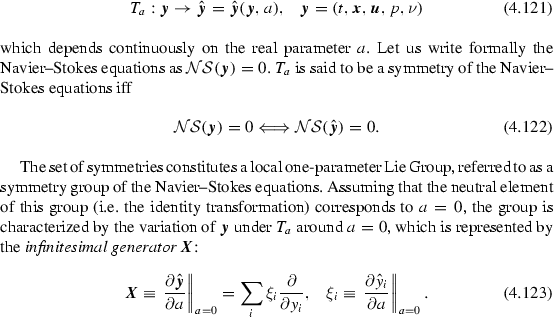
Once \(\varvec{X}\) is known, all elements of the symmetry group \(T_a\) can be calculated.
- 11.
An adequate choice for \(v^{\prime 2}_0\) yields \(v^{\prime 2}(t) = \mathcal{K}(t)\).
- 12.
- 13.
The value \(n=-1.38\) for \(\sigma =4\) is associated to a time varying Loitsyanski integral: \(\mathfrak {I}\sim t^{0.16}\). This results conflicts the most recent DNS results Ishida et al. (2006). This can be understood looking at the expansion of the nonlinear transfer term mediated by strongly non-local triadic interactions in the limit of very small wave numbers retrieved from two-point closures (e.g. EDQNM):
$$\begin{aligned} T(k \rightarrow 0)= \partial E/\partial t \sim A k^4 - 2 \nu _{turb} k^2 E, \end{aligned}$$where \(\nu _{turb}\) is an eddy viscosity. An error on the constant A may yield an error on the energy balance at very small wave numbers, inducing a spurious time-evolution of \(\mathfrak {I}\).
- 14.
One recognizes here \(\sqrt{\nu t}\) which is the similitude variable that appears in the dimensional analysis of the diffusive problems.
- 15.
This is consistent with the fact that it is the only solution which is fully consistent with the symmetry analysis at finite Reynolds number.
- 16.
Looking at previous results, such a theory should fill the gap that exists for \(0.1-1 \le Re_\lambda \le 100-300\).
- 17.
The Gâteaux derivative of a function \(\Psi \) at E in the direction F, with both E and F in the space spanned by the energy spectrum, is defined as:
$$ \langle \frac{\partial \Psi }{\partial E} (E), F \rangle = \left. \frac{\partial \Psi }{\partial E}\right| _{E}(F)=\lim \limits _{\epsilon \rightarrow 0} \frac{d}{d \epsilon }\Psi (E+\epsilon F). $$ - 18.
Weizsäcker and Heisenberg did not know the works of Oboukhov at this time.
- 19.
Thermalized is used here by analogy with the random molecular motion in which the macroscopic quantities such as temperature and pressure originate.
- 20.
While the observation of these structure is recent, it is worth noting that the idea that turbulent dissipation can be tied to a random distribution of vortex tubes and vortex sheets goes back to Townsend in 1951.
- 21.
This can be directly seen looking at the analytical expressions of the eigenvalues obtained for the Burgers vortex:
$$\begin{aligned} \hat{\lambda } _{\pm } = \frac{\alpha }{2} \left( -1 \pm Re_\Gamma \left( \frac{4 \nu }{\alpha r^2} \left( 1 - e^{ - \alpha r^2 / 4 \nu } \right) - e^{ - \alpha r^2 / 4 \nu } \right) \right) , \end{aligned}$$(4.364)$$\begin{aligned} \hat{\lambda } _z = \alpha , \end{aligned}$$(4.365)where \(Re_\Gamma = \Gamma / 4 \pi \nu \) is the circulation-based Reynolds number. If \(Re_\Gamma \) is high enough, the crossover between \(\hat{\lambda } _+\) and \(\hat{\lambda } _z\) occurs, i.e. there exists a region with \( \hat{\lambda } _+ \ge \hat{\lambda } _z\).
- 22.
These authors also define a strong vortex tube as a region with large vorticity and small strain rate.
- 23.
Another possible physical process for this scaling law, the interactions between vortex tubes, is shown to be much weaker than self-stretching.
- 24.
Uncoherent structures are defined here as structures with a characteristic vorticity weaker than the background vorticity \(\omega '\).
- 25.
High is to be understood as a relative notion, the reference being the wave numbers at which turbulent kinetic energy is injected/created by external forcing or hydrodynamic instabilities.
- 26.
In the one-dimensional case, the divergence-free constraint simplifies into a null space derivative constraint, leading to uniform solutions in space.
- 27.
Exact relations are \(u^{(1)} = - \hat{\omega }_\parallel /k\) and \(u^{(2)} = - \hat{u}_\parallel \) in the horizontal wave plane (\(k_\parallel =0\)).

References
André, J.-C., Lesieur, M.: Influence of helicity on the evolution of isotropic turbulence at high Reynolds number. J. Fluid Mech. 81, 187–207 (1977)
Andreotti, B.: Studying Burgers’ models to investigate the physical meaning of the alignments statistically observed in turbulence. Phys. Fluids 9, 735–742 (1997)
Antonia, R.A., Burattini, P.: Approach to the 4/5 law in homogeneous isotropic turbulence. J. Fluid Mech. 550, 175–184 (2006)
Bass, J.: Sur les bases mathématiques de la théorie de la turbulence. Comptes Rendus Acad. Sci. 228(3), 228–229 (1949)
Batchelor, G.K.: Energy decay and self-preserving correlation functions in isotropic turbulence. Q. Appl. Math. 6, 97 (1948)
Batchelor, G.K.: Pressure fluctuations in isotropic turbulence. Proc. Camb. Philos. Soc. 47, 359–374 (1951)
Batchelor, G.K.: The Theory of Homogeneous Turbulence. Cambridge University Press, Cambridge (1953)
Benney, D.J., Newell, A.C.: Random wave closure. Stud. Appl. Math. 48, 29–53 (1969)
Borue, V., Orszag, S.A.: Self similar decay of three-dimensional homogeneous turbulence with hyperviscosity. Phys. Rev. E 51(2), R856–R859 (1995a)
Borue, V., Orszag, S.A.: Forced three-dimensional homogeneous turbulence with hyperviscosity. Europhys. Lett. 29(9), 687–692 (1995b)
Bos, W.J.T., Bertoglio, J.-P.: Dynamics of spectrally truncated inviscid turbulence. Phys. Fluids 18, 071701 (2006a)
Bos, W.J.T., Bertoglio, J.-P.: A single-time two-point closure based on fluid particle displacements. Phys. Fluids 18, 031706 (2006b)
Bos, W.J.T., Rubinstein, R.: Dissipation in unsteady turbulence. Phys. Rev. Fluids 2, 022601(R) (2017)
Bos, W.J.T., Shao, L., Bertoglio, J.P.: Spectral imbalance and the normalized dissipation rate of turbulence. Phys. Fluids 19, 045101 (2007)
Brasseur, J.G., Wei, C.H.: Interscale dynamics and local isotropy in high Reynolds number turbulence within triadic interactions. Phys. Fluids 6(2), 842–870 (1994)
Cambon, C., Jacquin, L.: Spectral approach to non-isotropic turbulence subjected to rotation. J. Fluid Mech. 202, 295–317 (1989)
Cambon, C., Jeandel, D., Mathieu, M.: Spectral modelling of homogeneous non-isotropic turbulence. J. Fluid Mech. 104, 247–262 (1981)
Cantwell, B.J.: Exact solution of a restricted Euler equation for the velocity gradient tensor. Phys. Fluids A 4, 782–793 (1992)
Chakraborty, P., Balachandar, S., Adrian, R.J.: On the relationships between local vortex identification schemes. J. Fluid Mech. 535, 189–214 (2005)
Chandrasekhar, S.: The theory of statistical and isotropic turbulence. Phys. Rev. 76(5), 896–897 (1949)
Chertkov, M., Pumir, A., Shraiman, B.I.: Lagrangian tetrad dynamics and the phenomenology of turbulence. Phys. Fluids 11, 2394–2410 (1999)
Chevillard, L., Meneveau, C., Biferale, L., Toschi, F.: Modeling the pressure Hessian and viscous Laplacian in turbulence: comparisons with direct numerical simulation and implications on velocity gradient dynamics. Phys. Fluids 20, 101504 (2008)
Chong, M.S., Perry, A.E., Cantwell, B.J.: A general classification of three-dimensional flow fields. Phys. Fluids 2, 765–777 (1990)
Cichowlas, C., Bonati, P., Debbasch, F., Brachet, M.: Effective dissipation and turbulence in spectrally truncated Euler flows. Phys. Rev. Lett. 95, 264502 (2005)
Clark, T.T., Zemach, C.: Symmetries and the approach to statistical equilibrium in isotropic turbulence. Phys. Fluids 31, 2395–2397 (1998)
Clark, T.T., Rubinstein, R., Weinstock, J.: Reassessment of the classical turbulence closures: the Leith diffusion model. J. Turbul. 10(35), 1–23 (2009)
Coleman, G.N., Mansour, N.N.: Modeling the rapid spherical compression of isotropic turbulence. Phys. Fluids 3, 2255–2259 (1991)
Comte-Bellot, G., Corrsin, S.: The use of a contraction to improve the isotropy of grid-generated turbulence. J. Fluid Mech. 25, 657–682 (1966)
Davidson, P.A.: Turbulence. An Introduction for Scientists and Engineers. Oxford University Press, Oxford (2004)
Davidson, P.A.: The minimum energy decay rate in quasi-isotropic grid turbulence. Phys. Fluids 23, 085108 (2011)
De Divitiis, N.: von Karman-Howarth and Corrsin equations closure based on Lagrangian description of the fluid motion. Ann. Phys. 368, 296–309 (2016)
Djenidi, L., Antonia, R.A.: A general self-preservation analysis for decaying homogeneous isotropic turbulence. J. Fluid Mech. 773, 345–365 (2015)
Djenidi, L., Kamruzzaman, Md, Antonia, R.A.: Power-law exponent in the transition period of decay in grid turbulence. J. Fluid Mech. 779, 544–555 (2015)
Donzis, D.A., Sreenivasan, K.R., Yeung, P.K.: Some results on the Reynolds number scaling of pressure statistics in isotropic turbulence. Phys. D 241, 164–168 (2012)
Dryden, J.L.: A review of the statistical theory of turbulence. Q. Appl. Math. 1, 7–42 (1943)
Eyink, G.L., Thomson, D.J.: Free decay of turbulence and breakdown of self-similarity. Phys. Fluids 12(3), 477–479 (2000)
Favier, B., Godeferd, F.S., Cambon, C.: On space and time correlations of isotropic and rotating turbulence. Phys. Fluids 22, 015101 (2010)
Falkovich, G., Lebedev, V.: Single-point velocity distribution in turbulence. Phys. Rev. Lett. 79(21), 4159–4161 (1997)
Fjortoft, R.: On the changes in spectral distributions on kinetic energy for two-dimensional, non-divergent flow. Tellus 5, 225–230 (1953)
Fournier, J.D., Frisch, U.: \(d\)-dimensional turbulence. Phys. Rev. A 17(2), 747–762 (1978)
Frisch, U.: Turbulence: The Legacy of A. N. Kolmogorov. Cambridge University Press, Cambridge (1995)
George, W.K.: The decay of homogeneous turbulence. Phys. Fluids A 4(7), 1492–1509 (2000)
George, W.K.: Asymptotic effect of initial and upstream conditions on turbulence. ASME J. Fluids Eng. 134, 061203 (2012)
George, W.K., Wang, H.: The exponential decay of homogeneous isotropic turbulence. Phys. Fluids 21, 025108 (2000)
Girimaji, S.S., Zhou, Y.: Spectrum and energy transfer in steady Burgers turbulence. ICASE Report No. 95–13 (1995)
Goto, S., Vassilicos, J.C.: Energy dissipation and flux laws for unsteady turbulence. Phys. Lett. A 379, 1144–1148 (2015)
Guo, H., Li, C., Qu, Q., Liu, P.: Attractive fixed-point solution study of shell model for homogeneous isotropic turbulence. Appl. Math. Mech. 34, 259–268 (2013)
He, G.W., Jin, G., Zhao, X.: Scale-similarity model for Lagrangian velocity correlations in isotropic and stationary turbulence. Phys. Rev. E 80, 066313 (2009)
Heisenberg, W.: Zur statistischen theorie der turbulenz. Zeitschrift fur Physik 124, 628–657 (1948)
Hinze, J.O.: Turbulence. McGraw-Hill Series in Mechanical Engineering. McGraw-Hill, New York (1975)
Horiuti, K.: A classification method for vortex sheet and tube structures in turbulent flows. Phys. Fluids 13(12), 3756–3774 (2001)
Horiuti, K., Takagi, Y.: Identification method for vortex sheet structures in turbulent flows. Phys. Fluids 17, 121703 (2005)
Horiuti, K., Tamaki, T.: Nonequilibrium energy spectrum in the subgrid-scale one-equation model in large-eddy simulation. Phys. Fluids 25, 125104 (2013)
Horiuti, K., Yanagihara, S., Tamaki, T.: Nonequilibrium state in energy spectra and transfer with implications for topological transitions and SGS modeling. Fluid Dyn. Res. 48, 021409 (2016)
Hunt, J.C.R., Wray, A.A. Moin, P.: Eddies, stream, and convergence zones in turbulent flows. Center for Turbulence Research Report CTR-S88, pp. 193–208 (1988)
Ishida, T., Davidson, P.A., Kaneda, Y.: On the decay of isotropic turbulence. J. Fluid Mech. 564, 455–475 (2006)
Ishihara, T., Kaneda, Y., Yokokawa, M., Itakura, K., Uno, A.: Energy spectrum in the near dissipation range of high resolution DNS of turbulence. J. Phys. Soc. Jpn. 74(5), 1464–1471 (2005)
Jeong, J., Hussain, F.: On the identification of a vortex. J. Fluid Mech. 285, 69–94 (1995)
Jimenez, J.: Kinematic alignment effects in turbulent flows. Phys. Fluids 4, 652–654 (1992)
Jimenez, J., Wray, A.: On the characteristics of vortex filaments in isotropic turbulence. J. Fluid Mech. 373, 255–285 (1998)
Jimenez, J., Wray, A., Saffman, P.G., Rogallo, R.: The structure of intense vorticity in isotropic turbulence. J. Fluid Mech. 255, 65–90 (1993)
Kaneda, Y.: Lagrangian and Eulerian time correlations in turbulence. Phys. Fluids A 5(11), 2835–2845 (1993)
Kaneda, Y., Ishihara, T., Gotoh, K.: Taylor expansions in powers of time of Lagrangian and Eulerian two-point two-time velocity correlations in turbulence. Phys. Fluids 11, 2154–2166 (1999)
Kida, S., Ohkitani, K.: Spatiotemporal intermittency and instability of a forced turbulence. Phys. Fluids 4, 1018–1027 (1992a)
Kida, S., Ohkitani, K.: Fine structure of energy transfer in turbulence. Phys. Fluids 4, 1602–1604 (1992b)
Kovasznay, L.S.G.: The spectrum of locally isotropic turbulence. Phys. Rev. 73(9), 1115–1116 (1948)
Kraichnan, R.H.: The structure of isotropic turbulence at very high Reynolds numbers. J. Fluid Mech. 5(4), 497–543 (1959)
Kraichnan, R.H.: Inertial ranges in two-dimensional turbulence. Phys. Fluids 10, 1417–1423 (1967)
Kraichnan, R.H.: Inertial-range transfer in two- and three-dimensional turbulence. J. Fluid Mech. 47, 525–535 (1971)
Kraichnan, R.H.: Eddy-viscosity in two and three dimensions. J. Atmos. Sci 33, 1521–1536 (1976)
Kraichnan, R.H., Panda, R.: Depression of nonlinearity in decaying isotropic turbulence. Phys. Fluids 31, 2395–2397 (1988)
Krogstad, P.A., Davidson, P.A.: Near-field investigation of turbulence produced by multi-scale grids. Phys. Fluids 24, 035103 (2012)
Lamorgese, A.G., Caughey, D.A., Pope, S.B.: Direct numerical simulation of homogeneous turbulence with hyperviscosity. Phys. Fluids 17, 015106 (2005)
Lesieur, M.: Turbulence in fluids, 3rd edn. Kluwer Academic Publishers, Dordrecht (1997)
Lesieur, M., Schertzer, D.: Amortissement auto-similaire d’une turbulence à grand nombre de Reynolds. J. Méc. 17, 609–646 (1978). (in french)
Lesieur, M., Ossia, S., Metais, O.: Infrared pressure spectra in two- and three-dimensional isotropic incompressible turbulence. Phys. Fluids 11, 1535–1543 (1999)
Lindborg, E.: Correction to four-fifths law due to variations of the dissipation. Phys. Fluids 11(3) , 510–512 (1999)
Llor, A., Soulard, O.: Comment on “Energy spectra at low wavenumbers in homogeneous incompressible turbulence” (Phys. Lett. A 375, 2850 (2011)). Phys. Lett. A 377, 1157–1159 (2013)
Lund, T.S., Rogers, M.M.: An improved measure of strain rate probability in turbulent flows. Phys. Fluids 6, 1838–1847 (1994)
Lundgren, T.S.: Kolmogorov two-thirds law by matched asymptotic expansions. Phys. Fluids 14, 638–642 (2002)
Lundgren, T.S.: Kolmogorov turbulence by matched asymptotic expansion. Phys. Fluids 15, 1074–1081 (2003)
Manley, O.P.: The dissipation range spectrum. Phys. Fluids 4(6), 1320–1321 (1992)
Martins-Afonso, M., Meneveau, C.: Recent fluid deformation closure for velocity gradient tensor dynamics in turbulence: timescale effects and expansions. Phys. D 239, 1241–1250 (2010)
Mazzi, B., Vassilicos, J.C.: Fractal-generated turbulence. J. Fluid Mech. 502, 65–87 (2004)
Mathieu, J., Scott, J.: An Introduction to Turbulent Flow. Cambridge University Press, Cambridge (2000)
Martin, J., Dopazo, C., Valino, L.: Dynamics of velocity gradient invariants in turbulence: restricted Euler and linear diffusion models. Phys. Fluids 10, 2012–2025 (1998)
Mazellier, N., Vassilicos, J.C.: The turbulence dissipation constant is not universal because of its universal dependence on large-scale flow topology. Phys. Fluids 20, 015101 (2008)
Meldi, M., Sagaut, P.: On non-self similar regimes in homogeneous isotropic turbulence decay. J. Fluid Mech. 711, 364–393 (2012)
Meldi, M., Sagaut, P.: Further insights into self-similarity and self-preservation in freely decaying isotropic turbulence. J. Turbul. 14(8), 24–53 (2013a)
Meldi, M., Sagaut, P.: Pressure statistics in self-similar freely decaying isotropic turbulence. J. Fluid Mech. 717, R2-1–R2-12 (2013b)
Meldi, M., Sagaut, P.: Turbulence in a box: quantification of large-scale resolution effects in isotropic turbulence free decay. J. Fluid Mech. 818, 697–715 (2017)
Meldi, M., Sagaut, P., Lucor, D.: A stochastic view of isotropic turbulence decay. J. Fluid Mech. 668, 351–362 (2011)
Meldi, M., Lejemble, H., Sagaut, P.: On the emergence of non-classical decay regimes in multiscale/fractal generated isotropic turbulence. J. Fluid Mech. 756, 816–843 (2014)
Meneveau, C.: Lagrangian dynamics and models of the velocity gradient tensor in turbulent flows. Ann. Rev. Fluid Mech. 43, 219–245 (2011)
Meyers, J., Meneveau, C.: A functional form for the energy spectrum parametrizing bottleneck and intermittency effects. Phys. Fluids 20(6), 065109 (2008)
Millionschikov, M.D.: Theory of homogeneous isotropic turbulence. Dokl. Akad. Nauk. SSSR 32, 22–24 (1941)
Mohamed, M.S., Larue, J.C.: The decay power law in grid-generated turbulence. J. Fluid Mech. 219, 195–214 (1990)
Moisy, F.: Kolmogorov equation in a fully developed turbulence experiment. Phys. Rev. Lett. 82(20), 3994–3997 (1999)
Moisy, F., Jimenez, J.: Geometry and clustering of intense structures in isotropic turbulence. J. Fluid Mech. 513, 111–133 (2004)
Monin, A.S., Yaglom, A.M.: Statistical Fluid Mechanics, vol. 1. MIT Press, Cambridge (1975)
Mons, V., Chassaing, J.C., Gomez, T., Sagaut, P.: Is isotropic turbulence decay governed by asymptotic behavior of large scales? An eddy-damped quasi-normal Markovian-based data assimilation study. Phys. Fluids 26, 115105 (2014)
Nomura, K.K., Post, G.K.: The structure and the dynamics of vorticity and rate of strain in incompressible homogeneous turbulence. J. Fluid Mech. 377, 65–97 (1998)
Noullez, A., Pinton, J.F.: Global fluctuations in decaying Burgers turbulence. Eur. Phys. J. B. 28, 231–241 (2002)
Noullez, A., Vergassola, M.: A fast Legendre transfrom algorithm and applications to the adhesion model. J. Sci. Comput. 9(3), 259–281 (1994)
Noullez, A., Wallace, G., Lempert, W., Miles, R.B., Frisch, U.: Transverse velocity increments in turbulent flow using the RELIEF technique. J. Fluid Mech. 339, 287–307 (1997)
Noullez, A., Gurbatov, S.N., Aurell, E., Simdyankin, S.I.: Global picture of self-similar and non-self-similar decay in Burgers turbulence. Phys. Rev. E 71, 056305 (2005)
Oberlack, M.: On the decay exponent of isotropic turbulence. Proc. Appl. Math. Mech. 1, 294–297 (2002)
O’Brien, E.F., Francis, G.C.: A consequence of the zero fourth cumulant approximation. J. Fluid Mech. 13, 369–382 (1963)
Ogura, Y.: A consequence of the zero fourth cumulant approximation in the decay of isotropic turbulence. J. Fluid Mech. 16, 33–40 (1963)
Orszag, S.A.: Analytical theories of turbulence. J. Fluid Mech. 41, 363–386 (1970)
Park, N., Mahesh, K.: Analysis of statistical errors in large-eddy simulation using statistical closure theory. J. Comput. Phys. 222(1), 194–216 (2007)
Pao, Y.M.: Structure of turbulent velocity and scalar fields at large wavenumbers. Phys. Fluids 8(6), 1063–1075 (1965)
Piquet, J.: Turbulent flows. Models and Physics, 2nd edn. Springer, Berlin (2001)
Pope, S.B.: Turbulent Flows. Cambridge University Press, Cambridge (2000)
Pouquet, A., Lesieur, M., André, J.-C., Basdevant, C.: Evolution of high Reynolds number two-dimensional turbulence. J. Fluid Mech. 75, 305–319 (1975)
Qian, J.: Universal equilibrium range of turbulence. Phys. Fluids 27(9), 2229–2233 (1984)
Qian, J.: Slow decay of the finite Reynolds number effect of turbulence. Phys. Rev. E 60(3), 3409–3412 (1999)
Ristorcelli, J.R.: The self-preserving decay of isotropic turbulence: analytic solutions for energy and dissipation. Phys. Fluids 15, 3248–3250 (2003)
Ristorcelli, J.R.: Passive scalar mixing: analytic study of time scale ratio, variance, and mix rate. Phys. Fluids 18, 075101 (2006)
Ristorcelli, J.R., Livescu, D.: Decay of isotropic turbulence: fixed points and solutions for nonconstant \(G \sim R_\lambda \) palinstrophy. Phys. Fluids 16, 3487–3490 (2004)
Rossi, M.: Of vortices and vortical layers: an overview. In: Maurel, A., Petitjeans, P. (eds.) Vortex Structure and Dynamics. Lecture Notes in Physics, pp. 40–123. Springer, Berlin (2000)
Saffman, P.G.: On the fine scale structure of vector fields convected by a turbulent fluid. J. Fluid Mech. 16(4), 545–572 (1963)
Siggia, E.D.: Numerical study of small scale intermittency in three dimensional turbulence. J. Fluid Mech. 107, 375–406 (1981)
Skrbek, L., Stalp, S.R.: On the decay of homogeneous isotropic turbulence. Phys. Fluids 12(8), 1997–2019 (2000)
Speziale, C.G., Bernard, P.S.: The energy decay in self-preserving isotropic turbulence revisited. J. Fluid Mech. 241, 645–667 (1992)
Sreenivasan, K.R.: On the universality of the Kolmogorov constant. Phys. Fluids 7, 2778–2784 (1995)
Suzuki, E., Nakano, T., Takashi, N., Gotoh, T.: Energy transfer and intermittency in four-dimensional turbulence. Phys. Fluids 17, 081702 (2005)
Tanaka, M., Kida, S.: Characterization of vortex tubes and sheets. Phys. Fluids 5(9), 2079–2082 (1993)
Tatsumi, T.: The theory of decay process of incompressible isotropic turbulence. Proc. R. Soc. Lond. A 239, 16 (1957)
Taylor, G.I.: Statistical theory of turbulence. Proc. R. Soc. Lond. A 151, 421–444 (1935)
Tchoufag, J., Sagaut, P., Cambon, C.: A spectral approach to finite Reynolds number effects on Kolmogorov’s 4/5 law in isotropic turbulence. Phys. Fluids 24, 015107 (2012)
Thiesset, F., Antonia, R.A., Danaila, L., Djenidi, L.: Karman-Howarth closure equation on the basis of a universal eddy viscosity. Phys. Rev. E 88, 011003 (2013)
Tsinober, A.: An Informal Introduction to Turbulence. Kluwer Academic Publishers, Dordrecht (2001)
Vassilicos, J.C.: Dissipation in turbulent flows. Ann. Rev. Fluid Mech.47, 95–114 (2015)
Verzicco, R., Jimenez, J., Orlandi, P.: Steady columnar vortices under local compression. J. Fluid Mech. 299, 367–388 (1995)
Vignon, J.-M., Cambon, C.: Thermal spectral calculation using eddy-damped quasi-normal Markovian theory. Phys. Fluids 23, 1935–1937 (1980)
Von Karman, T., Howarth, L.: On the statistical theory of isotropic turbulence. Proc. R. Soc. A 164, 192–215 (1938)
Von Karman, T., Lin, C.C.: On the concept of similarity in the theory of isotropic turbulence. Rev. Mod. Phys. 21(3), 516–519 (1949)
Waleffe, F.: The nature of triad interactions in homogeneous turbulence. Phys. Fluids 4, 350–363 (1992)
Waleffe, F.: Inertial transfers in the helical decomposition. Phys. Fluids 5, 677–685 (1993)
Wilczek, M., Meneveau, M.: Pressure Hessian and viscous contributions to velocity gradient statistics based on Gaussian random fields. J. Fluid Mech. 756, 191–225 (2014)
Woodruff, S.L., Rubinstein, R.: Multiplescale perturbation analysis of slowly evolving turbulence. J. Fluid Mech. 565, 95–103 (2006)
Wylczek, M., Narita, Y.: Wave-number?frequency spectrum for turbulence from a random sweeping hypothesis with mean flow. Phys. Rev. E 86, 066308 (2012)
Zakharov, V.E., Lvov, V., Falkowitch, G.: Wave Turbulence. Springer, Berlin (1992)
Zhao, X., He, G.W.: Space-time correlations of fluctuating velocities in turbulent shear flows. Phys. Rev. E 79, 046316 (2009)
Zhou, J., Adrian, R.J., Balachandar, S., Kendall, T.M.: Mechanisms for generating coherent packets of hairpin vortices. J. Fluid Mech. 387, 353–396 (1999)
Author information
Authors and Affiliations
Corresponding author
Rights and permissions
Copyright information
© 2018 Springer International Publishing AG, part of Springer Nature
About this chapter

Cite this chapter
Sagaut, P., Cambon, C. (2018). Incompressible Homogeneous Isotropic Turbulence. In: Homogeneous Turbulence Dynamics. Springer, Cham. https://doi.org/10.1007/978-3-319-73162-9_4
Download citation
DOI: https://doi.org/10.1007/978-3-319-73162-9_4
Published:
Publisher Name: Springer, Cham
Print ISBN: 978-3-319-73161-2
Online ISBN: 978-3-319-73162-9
eBook Packages: Physics and AstronomyPhysics and Astronomy (R0)