Soft Subexponentials and Multiplexing

Abstract

Linear logic and its refinements have been used as a specification language for a number of deductive systems. This has been accomplished by carefully studying the structural restrictions of linear logic modalities. Examples of such refinements are subexponentials, light linear logic, and soft linear logic. We bring together these refinements of linear logic in a non-commutative setting. We introduce a non-commutative substructural system with subexponential modalities controlled by a minimalistic set of rules. Namely, we disallow the contraction and weakening rules for the exponential modality and introduce two primitive subexponentials. One of the subexponentials allows the multiplexing rule in the style of soft linear logic and light linear logic. The second subexponential provides the exchange rule. For this system, we construct a sequent calculus, establish cut elimination, and also provide a complete focused proof system. We illustrate the expressive power of this system by simulating Turing computations and categorial grammar parsing for compound sentences. Using the former, we prove undecidability results. The new system employs Lambek’s non-emptiness restriction, which is incompatible with the standard (sub)exponential setting. Lambek’s restriction is crucial for applications in linguistics: without this restriction, categorial grammars incorrectly mark some ungrammatical phrases as being correct.

1 Introduction

For the specification of deductive systems, linear logic [4, 5], and a number of refinements of linear logic have been proposed, such as commutative [23, 25] and non-commutative [11, 12] subexponentials, light linear logic [7], soft linear logic [16], and easy linear logic [10]. The key difference between these refinements is their treatment of the linear logic exponentials, !, ?. These refinements allow, e.g., a finer control on the structural rules, i.e., weakening, contraction and exchange rules, and how exponentials affect the sequent antecedent. For example [12], we proposed a logical framework with commutative and non-commutative subexponentials, applying it for applications in type-logical grammar. In particular, we demonstrated that this logical framework can be used to “type” correctly sentences that were not able before with previous logical frameworks, such as Lambek calculus.

However, as we have shown recently, our logical framework in [12] is incompatible with the important Lambek’s non-emptiness property [15]. This property, which requires all antecedents to be non-empty, is motivated by linguistic applications of Lambek-like calculi. Namely, it prevents the system from recognizing (“typing”) incorrectly formed sentences as grammatically correct. We discuss these linguistic issues in detail in Sect. 3. The lack of Lambek’s restriction means that the logical framework proposed in our previous work is too expressive, typing incorrectly sentences.

To address this problem, we propose a new non-commutative proof system, called $\mathsf {SLLM}$, that admits Lambek’s non-emptiness condition and at the same time is expressive enough to type correctly sentences in our previous work. This system is also still capable of modelling computational processes, as we show in Sect. 5.1 on the example of Turing computations.

In particular, $\mathsf {SLLM}$ takes inspiration from the following refinements of linear logic: subexponentials, by allowing two types of subexponentials, ! and $\nabla$; soft linear logic, which contributes a version of the multiplexing rule, $!_L$, shown below to the left; and light linear logic, which contributes the two right subexponentials rules, $!_R,\nabla _R$, shown below to the right.

In our version of the system, the premise of the rule $!_L$ does not allow zero instances of F. Hence, ! is a relevant subexponential as discussed in [12].

This rule is used to type sentences correctly, while the rules $!_R$ and $\nabla _R$ are used to maintain Lambek’s condition. $\mathsf {SLLM}$ contains, therefore, soft subexponentials and multiplexing.

Table 1. Lambek Calculus: A non-commutative version of ILL

Table 2. $\mathsf {SLLM}$: Lambek calculus with multiplexing.

Our main contributions are summarized below:

• Admissibility of Cut Rule: We introduce the proof system $\mathsf {SLLM}$ in Sect. 2. We also prove that it has basic properties, namely admissibility of Cut Rule and the substitution property. The challenge is to ensure a reasonable balance between the expressive power of systems and complexity of their implementation, and in particular, to circumvent the difficulties caused by linear logic contraction and weakening rules.

• Lambek’s Non-Emptiness Condition: We demonstrate in Sect. 3 that $\mathsf {SLLM}$ (and thus also $\mathsf {SLLMF}$) admits Lambek’s non-emptiness condition. This means that $\mathsf {SLLM}$ cannot be used to “type” incorrect sentences. We demonstrate this by means of some examples.

• Focused Proof System: We introduce in Sect. 4 a focused proof system ($\mathsf {SLLMF}$) proving that it is sound and complete with respect to $\mathsf {SLLM}$. The focused proof system differs from the focused proof system in our previous work [12] by allowing a subexponential that can contract, but not weaken nor be exchanged. Such subexponentials were not allowed in the proof system introduced in [12]. A key insight is to keep track on when a formula necessarily has to be introduced in a branch and when not.

• Complexity: We investigate in Sect. 5 the complexity of $\mathsf {SLLM}$. We first demonstrate that the provability problem for $\mathsf {SLLM}$ is undecidable in general and identify a fragment for which it is decidable.

Finally, in Sect. 6, we conclude by pointing to related and future work.

2 The Non-commutative System $\mathsf {SLLM}$ with Multiplexing

As the non-commutative source, we take the Lambek calculus [17], Table 1, the well-known fundamental system in linguistic foundations.

The proof system introduced here, $\mathsf {SLLM}$, extends the Lambek calculus by adding two new connectives (subexponentials) ! and $\nabla$ and their rules in Table 2.

Drawing inspiration from commutative logics such as linear logic [6], light linear logic [7], soft linear logic [16], and easy linear logic [10], here we introduce our primitive non-commutative modalities !A and $\nabla A$ controlled by a minimalistic set of rules.

Multiplexing Rule (local):

(1)

Informally, !A stands for: “any positive number of copies of A at the same position”.

Remark 1

In contrast to soft linear logic and light linear logic, where Weakening is one of the necessary ingredients, here we exclude the Weakening case: $(k = 0)$.

Unlike Contraction rule that can be recursively reused, and !A keeps the subexponential (it is introduced by Dereliction), our Multiplexing can only be used once with all copies provided immediately at the same time in one go, and the subexponentials get removed. Thus, if one wishes to reuse Multiplexing further in the proof, nested subexponentials would be needed (like !!A for two levels of Multiplexing).

The second subexponential, $\nabla A$, provides the exchange rule.

Exchange Rule (non-local):

(2)

and Dereliction Rule (local):

(3)

“$\nabla A$ can be thought of as storing a missing candidate A in a fixed local storage, with the ability to deliver A to the right place at the appropriate time.”

Remark 2

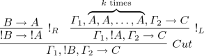
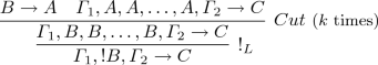
Notwithstanding that the traditional Promotion rule $\dfrac{\varGamma \rightarrow C}{{!}\varGamma \rightarrow {!}C}$ is accepted in linear logic as well as in soft linear logic, we confine ourselves to the restricted light linear logic promotion $\dfrac{A\rightarrow C}{{!}A\rightarrow {!}C}$, in order to guarantee cut admissibility for the non-commutative $\mathsf {SLLM}$ (cf. [11]). E.g., with $\dfrac{\varGamma \rightarrow C}{{!}\varGamma \rightarrow {!}C}$ the sequent

(4)

is derivable by cut

but, to finalize a cut-free proof for (4), we need commutativity:

The following theorem states that $\mathsf {SLLM}$ enjoys cut admissibility and the substitution property.

Theorem 1

 

• (a) The calculus $\mathsf {SLLM}$ enjoys admissibility of the Cut Rule:

  

  (5)

• (b) Given an atomic p, let the sequent be derivable in the calculus. Then for any formula B, is also derivable in the calculus. Here by $\varGamma (B)$ and C(B) we denote the result of replacing all occurrences of p by B in $\varGamma (p)$ and C(p), resp.

Proof.

• (a) By reductions. E.g.,

  

  is reduced to

  

• (b) By induction.

3 Linguistic Motivations

In this Section we illustrate how (and why) our modalities provide parsing complex and compound sentences in a natural language.

We start with standard examples, which go back to Lambek [17]; for in-depth discussion of linguistic matters we refer to standard textbooks [3, 19, 21].

The sentence “Bob sent the letter yesterday” is grammatical, and the following “type” specification is provable in Lambek calculus, Table 1.

$$ N, (N \mathop {\backslash }S) \mathop {/}N, N, V \mathop {\backslash }V \rightarrow S $$

Here the ‘syntactical type’ N stands for nouns “the letter” and “Bob”, and $((N\backslash S) / N)$, i.e., $(V / N)$, for the transitive verb “sent”, and $(V\backslash V)$ for the verb modifier “yesterday”, where $V = (N\backslash S)$. The whole sentence is of type S.

Lambek’s non-emptiness restriction is important for correctness of Lambek’s approach to modelling natural language syntax. Without this restriction Lambek grammars overgenerate, that is, recognize ungrammatical phrases as if they were correct. The standard example [19, § 2.5] is as follows: “very interesting book” is a correct noun phrase, established by the following derivation:

$$ (N \mathop {/}N) \mathop {/}(N \mathop {/}N), N \mathop {/}N, N \rightarrow N. $$

The sequent above is derivable in the Lambek calculus. Without Lambek’s restriction, however, one can also derive

$$ (N \mathop {/}N) \mathop {/}(N \mathop {/}N), N \rightarrow N $$

(since $\rightarrow N \mathop {/}N$ is derivable with an empty antecedent). This effect is unwanted, since the corresponding phrase “very book” is ungrammatical. Thus, Lambek’s non-emptiness restriction is a highly desired property for linguistic applications.

Fortunately, $\mathsf {SLLM}$ enjoys Lambek’s non-emptiness property. That is:

Theorem 2

The calculus $\mathsf {SLLM}$ provides Lambek’s non-emptiness restriction: If a sequent is derivable in the calculus then the list of formulas $\varGamma$ is not empty.

Proof

The crucial point is that, in the absence of Weakening, !A never happens to produce the empty list.    $\square$

Theorems 1 and 2 show how our new system $\mathsf {SLLM}$ resolves the issues discussed in [15] for the case of the Lambek calculus extended with a full-power exponential in linear logic style. Namely, as we show in that article, no reasonable extension of the Lambek calculus with the exponential modality can have the three properties simultaneously:

• cut elimination;

• substitution;

• Lambek’s restriction.

Moreover, as also shown in [15], for the one-variable fragment the same happens to the relevant subexponential, which allows contraction and permutation, but not weakening. Our new system overcomes these issues by refining the rules for subexponentials.

Now let us show how one can use subexponentials of $\mathsf {SLLM}$ to model more complicated sentences. Our analysis shares much with that of Morrill and Valentín [22]. Unlike ours, the systems in [22] do not enjoy Lambek’s restriction.

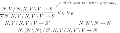
• (1) The noun phrase: “the letter that Bob sent yesterday,” is grammatical, so that its “type” specification (6) should be provable in Lambek calculus or alike:

  $$\begin{aligned} N, ((N \mathop {\backslash }N) \mathop {/}S'), N, (V \mathop {/}N), (V \mathop {\backslash }V) \rightarrow N \end{aligned}$$

  (6)

  Here $((N \mathop {\backslash }N) \mathop {/}S'$ stands for a subordinating connective “that”. As a type for the whole dependent clause,

  $$\begin{aligned} ``{Bob\,sent\,\_\,yesterday},'' \end{aligned}$$

  we take some $S'$, not a full S, because the direct object, “the letter”, is missing.

  Our solution refines the approach of [2, 20]. We mark the missing item, the direct object “the letter” of type N, by a specific formula $\nabla N$ stored at a fixed local position and by means of Exchange Rule (2) and Dereliction Rule (3) deliver the missing N to the right place with providing

  $$ N, (V \mathop {/}N), N, (V \mathop {\backslash }V) \rightarrow S,$$

  which is the type specification for the sentence “Bob sent the letter yesterday ” completed with the direct object, “the letter”. By taking $S' = (\nabla N\backslash S)$, we can prove (6):

  

Remark 3

If we allowed Weakening, we would prove the ungrammatical

“the letter that Bob sent the letter yesterday,”

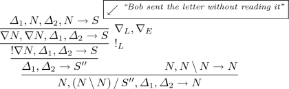
• (2) The noun phrase: “the letter that Bob sent without reading” is grammatical despite two missing items: the direct object to “sent” and the direct object to “reading”, resp. Hence, the corresponding “type” specification (7) should be provable in Lambek calculus or alike:

  $$\begin{aligned} N, ((N \mathop {\backslash }N) \mathop {/}S''), \varDelta _1, \varDelta _2 \rightarrow N \end{aligned}$$

  (7)

  Here N stands for “the letter”, and $((N \mathop {\backslash }N) \mathop {/}S'')$ for “that”, and some $\varDelta _1$ for “Bob sent”, and $\varDelta _2$ for “without reading”.

  As a type for the whole dependent clause,

  $$\begin{aligned} ``{Bob\,sent\,\_\,\_\,without\,reading\,\_\,\_ }\ '' \end{aligned}$$

  we have to take some $S''$, not a full S, to respect the fact that this time two items are missing: the direct objects to “sent” and “reading”, resp.

  To justify “the letter that Bob sent _ without reading _” with its (7), in addition to the $\nabla$-rules, we invoke Multiplexing Rule (1).

  The correlation between the full S and $S''$ with its multiple holes is given by:

  $$\begin{aligned} S'' = ((! \nabla N) \mathop {\backslash }S) \end{aligned}$$

  (8)

  As compared with the previous case of $S'$ representing one missing item $\nabla N$, the  $S''$ here is dealing with $!\nabla N$ which provides two copies of $\nabla N$ to represent two missing items.

  Then the proof for (7) is as:

  

4 Focused Proof System

This section introduces a sound and complete focused proof system $\mathsf {SLLMF}$ for $\mathsf {SLLM}$. Focusing [1] is a discipline on proofs that reduces proof search space. We take an intermediate step, by first introducing the proof system $\mathsf {SLLM\#}$ that handles the non-determinism caused by the multiplexing rule.

4.1 Handling Local Contraction

For bottom-up proof-search, the multiplexing rule

has a great deal of don’t know non-determinism as one has to decide how many copies of F appears in its premise. This decision affects provability as each formula has to be necessarily be used in the proof, i.e., they cannot be weakened.

To address this problem, we take a lazy approach by using two new connectives $\sharp ^*$ and $\sharp ^+$. The formula $\sharp ^* F$ denotes zero or more local copies of F, and $\sharp ^+ F$ one of more copies of F. We construct the proof system $\mathsf {SLLM\#}$ from $\mathsf {SLLM}$ as follows. It contains all rules of $\mathsf {SLLM}$, except the rule $!_L$, which is replaced by the following rules

Notice that there is no need for explicit contraction and only $\sharp ^*$ allows for weakening. We accommodate contraction into the introduction rules, namely, by modifying the rules where there is context splitting, such as in the rules $\mathop {\backslash }_L$. In particular, one should decide in which branch a formula C is necessarily be used. This is accomplished by using adequately $\sharp ^+ F$ and $\sharp ^* F$. For example, some rules for $\mathop {\backslash }_L$ are shown below:

In the first rule, the C is necessarily used in the right premise, while in the left premise one can chose to use C or not. $\mathsf {SLLM\#}$ contains similar symmetric rules where C is necessarily moved to the left premise. Also it contains the corresponding rules for $\mathop {/}_L$.

$\mathsf {SLLM\#}$ also include the following more refined right-introduction rules for ! and $\nabla$. where $\varGamma _1^*, \varGamma _2^*$ are lists containing only formulas of the form $\sharp ^* H$.

Notice how the decision that all formulas in $\varGamma _1, \varGamma _2$ represent zero copies is made in the rules above.

Theorem 3

Let $\varGamma ,G$ be a list of formulas not containing $\sharp ^*$ nor $\sharp ^+$. A sequent $\varGamma \rightarrow G$ is provable in the $\mathsf {SLLM}$ if and only if it is provable in $\mathsf {SLLM\#}$.

Completeness follows from straightforward proof by induction on the size of proofs. One needs to slightly generalize the inductive hypothesis. Soundness follows from the fact that contractions are local and can be permuted below every other rule.

4.2 Focused Proof System

First proposed by Andreoli [1] for Linear Logic, focused proof systems reduce proof search space by distinguishing rules which have don’t know non-determinism, classified as positive, from rules which have don’t care non-determinism, classified as negative. We classify the rules $\cdot _R, \mathop {\backslash }_L, \mathop {/}_L$ as positive and the rules $\cdot _L, \mathop {\backslash }_R, \mathop {/}_R$ as negative. Non-atomic formulas of the form $F \cdot G$ are classified as positive, $\nabla F, \sharp ^* F, \sharp ^+ F$ and !F are classified as modal formulas, and formulas of the form $F \mathop {\backslash }G$ and $F \mathop {/}G$ as negative.

The focused proof system manipulates the following types of sequents, where $\varGamma _1$ and $\varGamma _2$ are possibly empty lists of non-positive formulas, $\varTheta$ is multiset of formulas, and $N_N$ is a non-negative formula. Intitively, $\varTheta$ will contain all formulas of the form $\nabla F$. As they allow exchange rule, their collection can be treated as a multiset. $\varGamma _1, \varGamma _2$ contain formulas that cannot be introduced by negative rules.

• Negative Phase: $\varTheta : [\varGamma _1], {\Uparrow } \varDelta , [\varGamma _2] \rightarrow [N_N]$ and $\varTheta : [\varGamma _1], {\Uparrow } \varDelta , [\varGamma _2] \rightarrow {\Uparrow } F$. Intuitively, the formulas in $\varDelta$ and F are eagerly introduced whenever they negative rules are applicable, as one does not lose completeness in doing so.

• Border: $\varTheta : [\varGamma _1] \rightarrow [N_N]$. These are sequents for which no negative rule can be applied. At this moment, one has to decide on a formula starting a positive phase.

• Positive Phase: $\varTheta : [\varGamma _1], {\Downarrow } F, [\varGamma _2] \rightarrow [N_N]$ and $\varTheta : [\varGamma _1] \rightarrow {\Downarrow } F$, where only the formula F is focused on.

The focused proof system $\mathsf {SLLMF}$ is composed by the rules in Figs. 1 and 2. Intuitively, reaction rules $R_{L1}, R_{L2}, R_R$ and negative phase rules are applied until no more rules are applicable. Then a decision rule is applied which focuses on one formula. One needs, however, to be careful on whether the focused formula’s main connective is $\sharp ^+$ or $\sharp ^*$. If it is the former, then we have committed to one copy of the formula and therefore, it can be modified to be $\sharp ^*$, while the latter does not change.

The number of rules in Fig. 2 simply reflects the different cases emerging due to the presence or not of formulas whose main connective is $\sharp ^+$ or $\sharp ^*$. For example, $\mathop {\backslash }_{L2}$ considers the case when the splitting of the context occurs exactly on a formula $\sharp ^+ C$. In this case, the decision is to commit to use a copy of C in the right-premise, thus containing $\sharp ^+ C$, while $\sharp ^* C$ on the left-premise. The other rules follow the same reasoning.

Finally, notice that in the rules $I, !_R$ and $\nabla _R$ the context may contain formulas with main connective $\sharp ^*$ in their conclusion, but not in their premise. This illustrates the lazy decision of how many copies of a formula are needed.

Theorem 4

A sequent $\varGamma \rightarrow G$ is provable in $\mathsf {SLLM\#}$ if and only if the sequent $\cdot : {\Uparrow } \varGamma \rightarrow {\Uparrow } G$ is provable in $\mathsf {SLLMF}$.

The proof of this theorem follows the same ideas as detailed in [26] and [12].

Corollary 1

Let $\varGamma ,G$ be a list of formulas not containing $\sharp ^*$ nor $\sharp ^+$. A sequent $\varGamma \rightarrow G$ is provable in $\mathsf {SLLM}$ if and only if the sequent $\cdot : {\Uparrow } \varGamma \rightarrow {\Uparrow } G$ is provable in $\mathsf {SLLMF}$.

Remark 4

The focused proof system introduced above enables the use of more sophisticated search mechanisms. For example, lazy methods can reduce the non-determinism caused by the great number of introduction rules caused by managing $\sharp ^*,\sharp ^+$, e.g., Fig. 2.

Fig. 1.

Focused proof system for $\mathsf {SLLM\#}$. $N_N$ represent a non-negative formula. $N_{NA}$ represent a non-atomic, non-negative formula. $N_P$ represents a non-positive formula whose main connective is not $\nabla$. $N_P^\nabla$ represents a non-positive formula. We use $\mathcal {R}$ for both $\Uparrow G$ or $[N_N]$. We use $\sharp ^{+/*} F$ for both $\sharp ^{+} F$ and $\sharp ^{*} F$. We use $\varGamma ^*$ for a possibly empty list of formulas of the form $\sharp ^* F$.

5 Complexity

In this section, we investigate the complexity of $\mathsf {SLLM}$. In particular, we show that it is undecidable in general, by encoding Turing computations. This encoding also illustrate how the focused proof system $\mathsf {SLLMF}$ reduces non-determinism. We then identify decidable fragments for $\mathsf {SLLM}$.

5.1 Encoding Turing Computations in $\mathsf {SLLM}$

Any Turing instruction I is encoded by $!\nabla A_I$ with an appropriate $A_I$.

E.g., an instruction $I: q\xi \rightarrow q'\eta R$

if in state q looking at symbol $\xi$, replace it by $\eta$, move the tape head one cell to the right, and go into state $q'$,

is encoded by $!\nabla A_i$ where

$$ A_i = [(q_i\cdot \xi _i) \mathop {\backslash }(\eta _i\cdot q_i')] $$

Let M lead from an initial configuration, represented as $B_1\,\cdot \,q_1 \,\cdot \,\xi \,\cdot \,B_2$, to the final configuration $q_0$ (the tape is empty).

Fig. 2.

Focused left introduction rules for $\mathop {/}$ and $\mathop {\backslash }$ . The proviso $\star$ in $\mathop {\backslash }_{L1}$ states that the left-most formula of $\varGamma _2$ or the right-most formula of $\varGamma _1$ are not of the form $\sharp ^* F$ nor $\sharp ^+ F$. The proviso $\dagger$ in $\mathop {/}_{L1}$ is states that the right-most formula of $\varGamma _2$ or the left-most formula of $\varGamma _3$ are not of the form $\sharp ^* F$ nor $\sharp ^+ F$.

We demonstrate how focusing improves search with the encoding of Turing computations. For example, an instruction that write to the tape and moves to the right has the form: $A_i = [(q_i\cdot \xi _i) \mathop {\backslash }(\eta _i\cdot q_i')]$ while the Turing Machine (TM) configuration is encoded as in the sequent context: $[B_1, q_1, \xi , B_2]$ specifies A TM at state $q_1$ looking at the symbol $\xi$ in the tape $B_1, \xi , B_2$.

Assuming that $A_1, \ldots , A_n$ is used at least once, $!\nabla A_1, \ldots , !\nabla A_n$ specifies the behavior of the TM. This becomes transparent with focusing. The following focused derivation illustrate how a copy of an instruction encoding, below $A_1$, can be made available to be used. Recall that the one has to look at the derivation from bottom-up.

Notice that $A_1$ is placed in the $\varTheta$ context. This means that it can be moved at any place. Also notice that since one copy of $A_1$ is used, $\sharp ^+ \nabla A_1$ is replaced by $\sharp ^* \nabla A_1$.

The following derivation continues from the premise of the derivation above by focusing on $A_1$, $\mathcal {A}= \sharp ^*\nabla A_1, \ldots , !\nabla A_n$:

Notice that the resulting premise (at the right of the tree) specifies exactly the TM tape resulting from executing the instruction specified by $A_1$.

Moreover, notice that for the rule $D_4$, there are many options on where exactly to use $A_1$. However, it will only work if done as above. This is because otherwise it would not be possible to apply the initial rules as to the left of the derivation above. This reduces considerably the non-determinism involved for proof search.

Finally, once the final configuration $q_0$ (our Turing machine is responsible for garbage collection, so the configuration is just $q_0$, with no symbols on the tape) is reached, one finishes the proof:

The focusing discipline guarantees that the structure of the proof described above is the only one available. Therefore our encoding soundly and faithfully encodes Turing computations, resulting in the following theorem. However, notice additionally, that due to the non-determinism due to the ! left introduction, the encoding of Turing computations is not on the level of derivations, but on the level of proofs, following the terminology in [24].

The absence of Weakening seems to reduce the expressive power of our system $\mathsf {SLLM}$ in the case where not all instructions might have been applied within a particular computation, see Remark 5. However, we are still able to get a strong positive statement.

Theorem 5

We establish a strong correspondence between Turing computations and focused derivations in $\mathsf {SLLM}$.

Namely, given a subset $\{I_1, I_2, \dots , I_m\}$ of Turing instructions, the following two statements are equivalent:

• (a) The deterministic Turing machine M leads from an initial configuration, represented as $B_1\,\cdot \,q_1 \,\cdot \,\xi \,\cdot \,B_2$, to the final configuration $q_0$ so that $I_1$, $I_2$, ..., $I_m$ are only those instructions that have been actually applied in the given Turing computation.

• (b) A sequent of the following specified form is derivable in $\mathsf {SLLM}$.

  $$\begin{aligned} !\nabla A_{I_1},\,!\nabla A_{I_2},\,\dots ,\,!\nabla A_{I_m},\ B_1\,\cdot \,q_1\,\cdot \,\xi \,\cdot \,B_2\ \vdash \, {q_0} \end{aligned}$$

  (9)

Corollary 2

The derivability problem for $\mathsf {SLLM}$ is undecidable.

Proof

Assume the contrary: a decision algorithm $\alpha$ decides whether any sequent in $\mathsf {SLLM}$ is derivable or not. In particular, for any Turing machine M and any initial configuration of M, $\alpha$ decides whether any sequent of the form (9) is derivable or not, where $B_1\,\cdot \,q_1 \,\cdot \,\xi \,\cdot \,B_2$ represents the initial configuration.

Then for each of the subsets $\{I_1, I_2, \dots , I_m\}$ of the instructions of M, we apply $\alpha$ to the corresponding sequent of the form (9).

If all results are negative then we can conclude that M does not terminate on the initial configuration, represented as $B_1\,\cdot \,q_1 \,\cdot \,\xi \,\cdot \,B_2$.

Otherwise, M does terminate.

Since the halting problem for Turing machines is undecidable, we conclude that $\alpha$ is impossible.    $\square$

Remark 5

The traditional approach to machine-based undecidability is to establish a one-to-one correspondence between machine computations and derivations in the system under consideration. Namely, given a Turing/Minsky machine M, we encode M as a formula $\mathtt{code}_M$, the ‘product’ of all $C_I$ representing instructions I. The ‘product’ ranges over all M’s instructions. Then we have to establish that, whatever initial configuration W we take, a sequent of the form

$$\begin{aligned} \mathtt{code}_M, \, W \, \vdash \, {q_0} \end{aligned}$$

(10)

is decidable in the logical system at hand iff M terminates on the initial configuration represented as W. Here one and the same $\mathtt{code}_M$ is used for each of the initials W.

Now, suppose that M terminates on each of the initial configurations $W_1$ and $W_2$ so that some instruction represented by $\widetilde{C}$ is used within the computation starting with $W_1$, but it is not used within the computation starting with $W_2$. Then, because of $W_1$, $\widetilde{C}$ takes an active part within $\mathtt{code}_M$. On the other hand, $\widetilde{C}$ becomes redundant and must be ‘ignored’ within the derivation for the sequent $\mathtt{code}_M,W_2 \vdash \,{q_0}$. To cope with the problem, it would be enough, e.g., to assume Weakening in the system under consideration, which is not a case here.

The novelty of our approach to the machine-based undecidability is to circumvent the problem caused by the absence of Weakening, by changing the order of quantifiers.

Instead of $\mathtt{code}_M$, one and the same for all W, we introduce a finite number of candidates of the form (9) with ranging over subsets $\{I_1, I_2, \dots , I_m\}$ of the instructions of M.

According to Theorem 5, for any initial configuration W, there exists a sequent, say $\mathtt{code}_{M,W}, W \vdash \,{q_0}$, chosen from the finite set of candidates of the form (9) such that the terminated computation starting from W corresponds to an $\mathsf {SLLM}$ derivation for the chosen $\mathtt{code}_{M,W}, W \vdash \,{q_0}$. See also Corollary 2.    $\square$

5.2 Decidable Fragments: Syntactically Defined

An advantage of our approach is that, unlike the contraction rule, we can syntactically control the multiplexing to provide decidable fragments still sufficient for applications.

Theorem 6

If we bound k in the multiplexing rule in the calculus $\mathsf {SLLM}$ with a fixed constant $k_0$, such a fragment becomes decidable.

Proof Sketch. Each application of Multiplexing of the form:

multiplies the number of formulas with the factor $k_0$, which provides an upper bound on the size S of the sequents involved:

$$ S = O(S_0\cdot k_0^n) $$

here $S_0$ is the size of the input, and n is a bound on the nesting depth of the !-formulas. It suffices to apply a non-deterministic decision procedure but generally on the sequents of exponential size.    $\square$

Theorem 7

In the case where we bound k in the multiplexing rule in the calculus $\mathsf {SLLM}$ with a fixed constant $k_0$, and, in addition, we bound the depth of nesting of !A, we get NP-completeness.

Remark 6

In fact Theorem 7 gives NP-procedures for parsing complex and compound sentences in many practically important cases.

Remark 7

The strong lower bound is given by the following.

The !-free fragment that invokes only one implication, $(A\backslash B)$, and $\nabla A$ is still NP-complete.

6 Concluding Remarks

In this paper we have introduced $\mathsf {SLLM}$, a non-commutative intuitionistic linear logic system with two subexponentials. One subexponential implements permutation and the other one obeys the multiplexing rule, which is a weaker, miniature version of contraction. Our system was inspired by subexponentials [23], linear logic [6], light linear logic [7], soft linear logic [16], and easy linear logic [10].

We have also provided a complete focused proof system for our calculus $\mathsf {SLLM}$. We have illustrated the expressive power of the focused system by modelling computational processes.

The general aim is to develop more refined and efficient procedures for the miniature versions of non-commutative systems, e.g., Lambek calculus and its extensions, based on the multiplexing rule. We aim to ensure a reasonable balance between the expressive power of the formal systems in question and the complexity of their algorithmic implementation. The calculus $\mathsf {SLLM}$, with multiplexing instead of contraction, provides simultaneously three properties: cut elimination, substitution, and Lambek’s restriction.

One particular advantage of our system $\mathsf {SLLM}$ to systems in our previous work [12, 15] is the fact that it naturally incorporates Lambek’s non-emptiness restriction, which is incompatible with stronger systems involving contraction [15]. Lambek’s non-emptiness restriction plays a crucial role in applications of substructural (Lambek-style) calculi in formal linguistics (type-logical grammars). Indeed, overcoming this impossibility result is one of our main motivations in looking for a system that would satisfy cut-elimination, substitution, and the Lambek’s restriction. The new system proposed in this paper is our proposed solution to this subtle and challenging problem.

Moreover, there is no direct way of reducing the undecidability result in this paper, say, to the undecidability results from our previous papers [11, 14, 15] by a logical translation or representation of the logical systems. Since a number of those systems are also undecidable, there are of course Turing reductions both ways to the system in this paper. However, the Turing reductions factor through the new representation of Turing machines introduced in this paper. That is, the undecidability result in this paper is a new result.

Also the focused proof system proposed here has innovations to the paper [12]. For example, our proof system contains relevant subexponentials that do not allow contraction, something that was not addressed in [12]. Indeed such subexponentials have also been left out of other focused proof systems, e.g., in the papers [23, 25].

Another advantage of this approach is that, unlike the contraction rule, we can syntactically control the multiplexing to provide feasible fragments still sufficient for linguistic applications.

As future work, we plan to investigate how to extend the systems proposed in this paper with additives. In particular, the proposed focused proof system using the introduced connectives $\sharp ^*,\sharp ^+$ may have to be extended in order to support additives. This is because it seems problematic, with these connectives, to provide that the same number of copies of a contractable formula are used in both premises when introducing an additive connective.

Financial Support. The work of Max Kanovich was partially supported by EPSRC Programme Grant EP/R006865/1: “Interface Reasoning for Interacting Systems (IRIS).” The work of Andre Scedrov and Stepan Kuznetsov was prepared within the framework of the HSE University Basic Research Program and partially funded by the Russian Academic Excellence Project ‘5–100’. The work of Stepan Kuznetsov was also partially supported by grant MK-430.2019.1 of the President of Russia, by the Young Russian Mathematics Award, and by the Russian Foundation for Basic Research grant 20-01-00435. Vivek Nigam’s participation in this project has received funding from the European Union’s Horizon 2020 research and innovation programme under grant agreement No 830892. Vivek Nigam is also partially supported by CNPq grant 303909/2018-8.

References

Andreoli, J.-M.: Logic programming with focusing proofs in linear logic. J. Log. Comput. 2(3), 297–347 (1992)
Barry, G., Hepple, M., Leslie, N., Morrill, G.: Proof figures and structural operators for categorial grammar. In: Proceedings of the Fifth Conference of the European Chapter of the Association for Computational Linguistics, Berlin (1991)
Carpenter, B.: Type-Logical Semantics. MIT Press, Cambridge (1998)
Cervesato, I., Pfenning, F.: A linear logic framework. In: Proceedings of the Eleventh Annual IEEE Symposium on Logic in Computer Science, New Brunswick, New Jersey, pp. 264–275. IEEE Computer Society Press, July 1996
Cervesato, I., Pfenning, F.: A linear logical framework. Inform. Comput. 179(1), 19–75 (2002)
Girard, J.-Y.: Linear logic. Theor. Comput. Sci. 50(1), 1–101 (1987)
Girard, J.-Y.: Light linear logic. Inform. Comput. 143(2), 175–204 (1998)
Kanovich, M.I.: Horn programming in linear logic is NP-complete. In: Proceedings of the Seventh Annual IEEE Symposium on Logic in Computer Science , pp. 200–210 (1992)
Kanovich, M.I., Okada, M., Scedrov, A.: Phase semantics for light linear logic. Theor. Comput. Sci. 294(3), 525–549 (2003)
Kanovich, M.I.: Light linear logics with controlled weakening: expressibility, confluent strong normalization. Ann. Pure Appl. Logic 163(7), 854–874 (2012)
Kanovich, M., Kuznetsov, S., Nigam, V., Scedrov, A.: Subexponentials in non-commutative linear logic. Math. Struct. Comput. Sci. 29(8), 1217–1249 (2019)
Kanovich, M., Kuznetsov, S., Nigam, V., Scedrov, A.: A logical framework with commutative and non-commutative subexponentials. In: Galmiche, D., Schulz, S., Sebastiani, R. (eds.) IJCAR 2018. LNCS (LNAI), vol. 10900, pp. 228–245. Springer, Cham (2018). https://doi.org/10.1007/978-3-319-94205-6_16
Kanovich, M., Kuznetsov, S., Scedrov, A.: L-models and R-models for Lambek calculus enriched with additives and the multiplicative unit. In: Iemhoff, R., Moortgat, M., de Queiroz, R. (eds.) WoLLIC 2019. LNCS, vol. 11541, pp. 373–391. Springer, Heidelberg (2019). https://doi.org/10.1007/978-3-662-59533-6_23
Kanovich, M., Kuznetsov, S., Scedrov, A.: Undecidability of the Lambek calculus with a relevant modality. In: Foret, A., Morrill, G., Muskens, R., Osswald, R., Pogodalla, S. (eds.) FG 2015-2016. LNCS, vol. 9804, pp. 240–256. Springer, Heidelberg (2016). https://doi.org/10.1007/978-3-662-53042-9_14
Kanovich, M., Kuznetsov, S., Scedrov, A.: Reconciling Lambek’s restriction, cut-elimination, and substitution in the presence of exponential modalities. J. Logic Comput. 30(1), 239–256 (2020)
Lafont, Y.: Soft linear logic and polynomial time. Theor. Comput. Sci. 318(1–2), 163–180 (2004)
Lambek, J.: The mathematics of sentence structure. Amer. Math. Monthly 65(3), 154–170 (1958)
Lincoln, P., Mitchell, J.C., Scedrov, A., Shankar, N.: Decision problems for propositional linear logic. Ann. Pure Appl. Logic 56(1–3), 239–311 (1992)
Moot, R., Retoré, C.: The Logic of Categorial Grammars. A Deductive Account of Natural Language Syntax and Semantics. LNCS vol. 6850. Springer, Cham (2012). https://doi.org/10.1007/978-3-642-31555-8
Moortgat, M.: Constants of grammatical reasoning. In: Bouma, G., Hinrichs, E., Kruijff, G.-J., Oehrle, R. (eds.) Constraints and Resources in Natural Language Syntax and Semantics, pp. 195–219. CSLI Publications, Stanford (1999)
Morrill, G.: Categorial Grammar: Logical Syntax, Semantics, and Processing. Oxford University Press, Oxford (2011)
Morrill, G., Valentín, O.: Computational coverage of TLG: nonlinearity. In: Kanazawa, M., Moss, L., de Paiva, V. (eds.) Proceedings of NLCS 2015. Third Workshop on Natural Language and Computer Science, EPiC, vol. 32, pp. 51–63. EasyChair (2015)
Nigam, N., Miller, D.: Algorithmic specifications in linear logic with subexponentials. In: Proceedings of the 11th ACM Sigplan Conference on Principles and Practice of Declarative Programming, pp. 129–140 (2009)
Nigam, V., Miller, D.: A framework for proof systems. J. Automated Reason. 45(2), 157–188 (2010)
Nigam, V., Pimentel, E., Reis, G.: An extended framework for specifying and reasoning about proof systems. J. Logic Comput. 26(2), 539–576 (2016)
Saurin, A.: Une étude logique du contrôle. Ph.D. Thesis (2008)
Yetter, D.N.: Quantales and (noncommutative) linear logic. J. Symb. Log. 55(1), 41–64 (1990)
Author information
Authors and Affiliations
Corresponding author
Editor information
Editors and Affiliations
Rights and permissions
Copyright information
© 2020 Springer Nature Switzerland AG
About this paper
Cite this paper
Kanovich, M., Kuznetsov, S., Nigam, V., Scedrov, A. (2020). Soft Subexponentials and Multiplexing. In: Peltier, N., Sofronie-Stokkermans, V. (eds) Automated Reasoning. IJCAR 2020. Lecture Notes in Computer Science(), vol 12166. Springer, Cham. https://doi.org/10.1007/978-3-030-51074-9_29
Download citation
DOI: https://doi.org/10.1007/978-3-030-51074-9_29
Published:
Publisher Name: Springer, Cham
Print ISBN: 978-3-030-51073-2
Online ISBN: 978-3-030-51074-9
eBook Packages: Computer ScienceComputer Science (R0)