Modeling Multiphase Flow and Heat Transfer

Abstract

This chapter presents the generalized macroscopic (integral) and microscopic (differential) conservation equations for multiphase systems for both local-instance and averaged formulations. The instantaneous formulation requires a differential balance for each phase, combined with appropriate jump and boundary conditions to match the solution of these governing equations at the interfaces. The averaged formulations are obtained by averaging the governing conservation equations within a small time-interval (time average) or a small control volume (spatial average). The governing conservation equations for the multidimensional, multi-fluid, homogeneous, mixture and separated models are also discussed as well as area-averaged governing conservation equations for one-dimensional flows.

Problems

• 3.1. The local instance continuity equation can also be obtained by performing a mass balance for the differential control volume shown in Fig. P3.1. Derive the continuity equation and compare your result with Eq. (3.51).

  

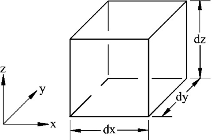
  Fig. P3.1

• 3.2. Derive the local instance continuity equation in a cylindrical coordinate system using the control volume shown in Fig. P3.2.

  

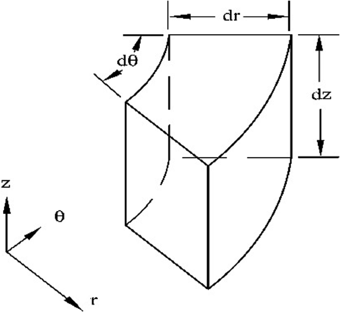
  Fig. P3.2

• 3.3. The continuity equation for incompressible flow is Eq. (3.52). Is it valid for transient flow? Why or why not?

• 3.4. In order to take water without stopping the train, a narrow trough of several thousand feet long can be placed in the midway between the rails of a railroad track. As a locomotive passes over the narrow trough, the water can be forced up into the tender through a scoop by the speed of the locomotive (see Fig. P3.4). Assuming the cross-sectional area of the scoop is A, find the force acting on the train by the water using momentum balance in (a) a coordinate system that is attached to and moves with the locomotive, and (b) a fixed coordinate system.

  

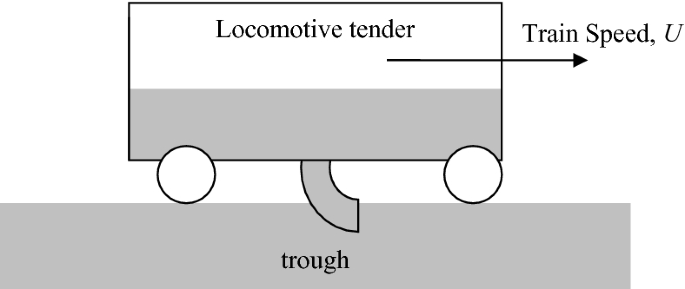
  Fig. P3.4

• 3.5. Use the integral form of the energy equation to calculate the steady mass flow rate of water in a pump that delivers 4 horsepower to the fluid, as given in Fig. P3.5, for the control volume shown. The pump inlet and outlet diameters are 10. and 4 in., respectively.

  

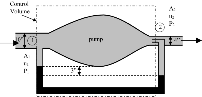
  Fig. P3.5

• 3.6. Consider a liquid heated in an upward flow configuration in a vertical 10-m-long tube of constant diameter. The inlet average velocity and pressure are 2 m/s and 350 kPa, respectively. Determine the heat needed to be added to the fluid so that the losses in internal energy equal 180 kJ/kg. Assume the density is 1000 kg/m³ and outlet pressure is 1 atm.

• 3.7. Water flows through a 3-in.-diameter pipe at a rate of 45 gal/min. Frictional forces produce a pressure drop of 8 psi. Determine the temperature change of the water if the heat transfer to the pipe can be neglected.

• 3.8. Determine the change in water temperature before (1) and (3) in terms of the inlet parameters A₁, A₂, u₁, u₂, c_v, and θ for the configuration shown in Fig. P3.8. Assume T₁ = T₂ and $p_{1} = p_{2}$. The change in internal energy can be approximated as de = c_vdT.

  

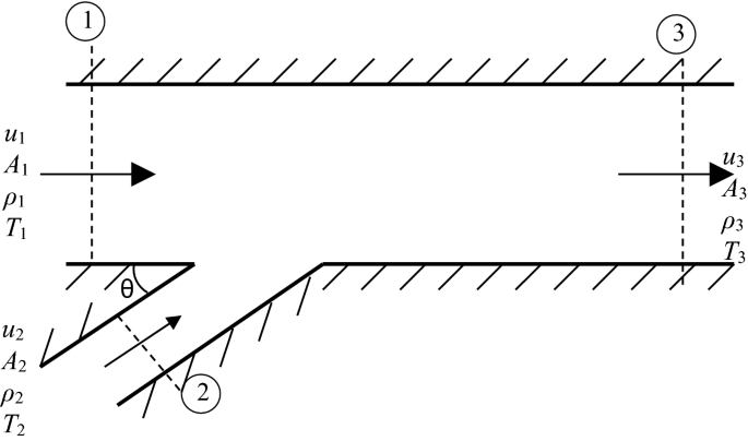
  Fig. P3.8

• 3.9. Gas enters an insulated tank with total volume V through a pipe with diameter D with an inlet velocity and temperature of u_i and T_i, respectively, as shown in Fig. P3.9. Using the integral form of the energy equation, determine a first-order equation for the rate of change in temperature in the tank as a function of (V, D, u_i, T_i).

  

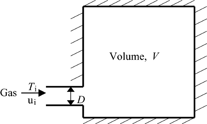
  Fig. P3.9

• 3.10. Determine viscous dissipation for compressible flow in the Cartesian coordinate system.

• 3.11. Write down the governing equations for two-dimensional, compressible flow with the effect of viscosity being accounted for in a Cartesian coordinate system. Assume that the constant properties assumptions apply and that the only body force is gravity.

• 3.12. Fourier’s law of conduction [see Eq. (1.22)] assumes that heat flux responds immediately to a temperature gradient. However, for cases with a very high temperature gradient or extremely short duration, heat is propagated at a finite speed, which can be accounted for by a modified heat flux model:

  $$ {\mathbf{q}^{\prime\prime}} + \tau \frac{{\partial {\mathbf{q}^{\prime\prime}}}}{\partial t} = - k\nabla T $$

  where $\tau$ is the thermal relaxation time. Derive the energy equation for a pure substance using the above model and Eq. (3.90). Internal heat generation and viscous dissipation can be neglected.

• 3.13. The enthalpy for the ith component is $h_{i}$ is function of temperature, T, and pressure , p. Show that the substantial derivative in terms of the velocity of the ith component, V_i, can be obtained from Eq. (3.162).

• 3.14. Formulate the hydrodynamics for developing flow in a duct formed by two infinite flat plates. Assume the flow to be laminar, incompressible, 2D, and steady. It can also be assumed that the inlet velocity at the entrance of the duct is uniform, as shown in Fig. P3.14. Using the integral method, find out the hydrodynamic entrance and the skin friction coefficient in terms of Reynolds number. Is the analysis valid for a circular pipe?

  

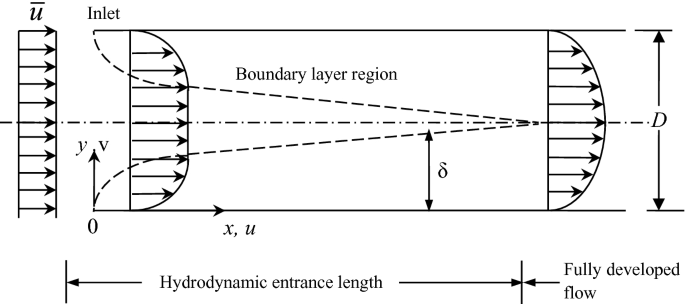
  Fig. P3.14

• 3.15. Formulate the hydrodynamics when flow is fully developed in a duct formed by two infinite flat plates and a round pipe. Assume the flow to be laminar, incompressible, two-dimensional, and steady. Because flow is fully developed, it can be assumed that the velocity in the duct does not change in the x-direction. Determine the skin friction coefficient . Clearly, describe the methods used to solve the momentum and continuity equations.

• 3.16. Obtain the Nusselt number for constant wall temperature and constant wall heat flux cases for fully developed flow in terms of temperature and velocity profiles in a circular pipe. Assume laminar, incompressible, two-dimensional, and steady state.

• 3.17. Develop analytical expressions for the Nusselt number for constant wall temperature and constant heat flux cases in a circular pipe with a fully developed velocity profile but a developing temperature profile. Assume laminar, incompressible, two-dimensional, and steady state with uniform inlet velocity.

• 3.18. Consider steady-state, two-dimensional, fully developed thermal and hydrodynamic laminar flow with constant properties in a circular pipe. Let there be heat transfer to or from the fluid at a constant rate per unit of tube length. Determine the Nusselt number if the effect of frictional heating due to viscosity (viscous dissipation ) is included in the analysis. How does frictional heating affect the Nusselt number ? Identify the pertinent nondimensional parameters appearing in this problem.

• 3.19. The Couette flow was discussed in Example 3.4. When both surfaces are stationary and flow is caused by an applied pressure gradient in the x-direction, dp/dx, it is called Poiseuille flow (see Fig. P3.19). The fluid is Newtonian and incompressible. Temperature in the upper and lower plates is kept constant at T₁ and T₂, respectively. Determine the fluid temperature distribution and heat flux with the following assumptions (Poiseuille flow): (1) steady state, (2) constant properties, (3) laminar flow, (4) constant ∂p/∂x, (5) no end effects, (6) no edge effects, and (7) gravity is the only body force.

  

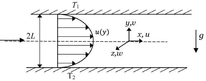
  Fig. P3.19

• 3.20. Consider the steady flow of an incompressible fluid making an angle θ with the vertical direction with constant liquid film thickness $\delta$ along an inclined flat surface with length L and width W as shown in Fig. P3.20. Determine the average velocity, volumetric flow rate, film thickness $\delta$, and the force of the fluid on the surface . Neglect the end, exit, and edge effects and assume constant properties. The air is stagnant next to the liquid free surface .

  

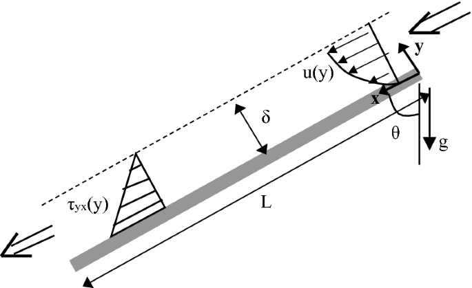
  Fig. P3.20

• 3.21. Develop the energy equation and boundary conditions, for Problem 3.20 for the case of constant wall temperature T_w and uniform inlet temperature T₀. Determine the temperature distribution and heat transfer rate for the wall to film for start-up period (short contact time) that the fluid temperature changes only in the vicinity of the wall.

• 3.22. Develop formulation for the case of heating with no evaporation for the flow over a rotating disk (Fig. P3.22) Assume that the flow is laminar, incompressible, steady, axisymmetric, and the disk has a constant wall temperature. The flow is introduced from a central collar that directs the liquid radially outward with velocity u₀ over a gap height of h₀. $\delta$ is the liquid film thickness and r₀ is the initial radius of the disk at the outlet of the collar, h₀ is the collar height and $\delta{T}$ is the thickness of the thermal boundary layer. Obtain Nusselt number $Nu = hr_{0} /k,$ and film thickness $\delta /h_{0}$ as a function of the Reynolds number and Rossby numbers $[Re = u_{0} r_{0} /\nu$ and ${Ro} = u_{0}^{2} /(\omega^{2} r_{0}^{2} )]$ using the integral method.

  

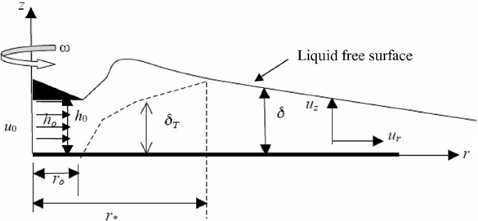
  Fig. P3.22

• 3.23. Derive the continuity equation at a liquid–vapor interface , Eq. (3.174), by considering conservation of mass for a control volume that includes two phases as given by Eq. (3.8) with $\Pi = 2$.

• 3.24. Eq. (3.174) is valid for an interface between liquid and vapor phases . Derive the conservation of mass for solid–liquid interface that is applicable to the melting problem.

• 3.25. Derive the momentum equation at an interface, Eq. (3.176), from the integral momentum equation for a control volume containing two phases separated by an interface as given by Eq. (3.13) with $\Pi = 2$.

• 3.26. Derive the energy equation at an interface, Eq. (3.177), from the integral energy equation for a control volume containing two phases separated by an interface as given by Eq. (3.23) with $\Pi = 2$.

• 3.27. The momentum balance equation at a three-dimensional interface was discussed in Sect. 3.3.6. Derive the momentum balance equation for a two-dimensional interface between phases 1 and 2. The effect of surface tension can be neglected.

• 3.28. A tube with radius R_o and zero thickness passes through a liquid phase-change material at its melting point, T_m (see Fig. P3.28). A cold fluid with a temperature of T_c, which is below T_m, flows through the inside of the tube. Solidification will occur on the outer surface of the tube. Formulate the problem by giving the governing equations and corresponding boundary conditions in the cylindrical coordinate system. If the problem can be assumed to be quasi-steady state, solve for the instantaneous location of the solid–liquid interface .

  

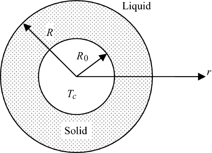
  Fig. P3.28

• 3.29. The time it takes to completely burn a fuel droplet of specified size as estimated by Eq. (3.242) is valid for conduction -controlled combustion processes. For a liquid droplet that has sufficient inertia, the heat transfer between vapor and liquid is dominated by convection , i.e., Equation (3.236) is replaced by $\dot{m}^{\prime\prime}_{\text{f}} h_{{\ell \text{v}}} = q_{\text{I}}^{\prime \prime } = h\theta_{\infty }$, where h is the heat transfer coefficient between the gaseous mixture and liquid droplet, and can be obtained by $Nu_{D} = hD/k = CRe_{D}^{1/2}$. What is the time it takes to completely burn the liquid fuel droplet ? Compare your result with Eq. (3.242).

• 3.30. Redo Example 3.7 using the result from Problem 3.29 and compare your result with the result in Example 3.7. The relative velocity of the fuel droplet is $V_{\text{p}} = 5\,\text{m}/\text{s}$, and the heat transfer correlation is $Nu_{D} = 0.6Re_{D}^{1/2}$. The viscosity of the gaseous mixture is $4 \times 10^{ - 5}\,\text{m}^{2} /\text{s}$.

• 3.31. A fuel droplet with an initial diameter of D_p moves at a velocity v_p in an oxidant gas. The gravitational acceleration vector is g, and the local oxidant gas velocity vector is v_g. The fuel droplet evaporates as it moves in the combustor. If the drag coefficient of the fuel droplet is C_D, write the momentum equation for the fuel droplet.

• 3.32. If the temperature of the fuel droplet in Problem 3.31 can be assumed to be uniform at any time, and the latent heat of evaporation of the fuel is $h_{{\text{s}\ell }}$, derive the energy equation for the fuel droplet.

• 3.33. A saturated mixture of water and its vapor at 180 °C flows in a 0.1 m ID tube with a mass flow rate of 0.5 kg/s. The liquid water is dispersed in the vapor phase in the form of 0.1-mm-diameter droplets, and the quality of the mixture is x = 0.75. The average velocity of the vapor phase is 30 m/s. Find (a) the average velocity of the liquid droplets and (b) the interactive force between the liquid and vapor phase.

• 3.34. If the liquid droplet is subcooled at a temperature of 175 °C, estimate the interphase heat transfer rate between liquid and vapor phases in the above problem.

• 3.35. The mass flux in the channel is defined as the mass flow rate per unit area. What is the total mass flow rate for the multiphase flow discussed in Example 3.10?

• 3.36. Consider flow entering from different sides of a tee-junction in a duct. The fluid entering is a mixture of air and liquid water, with known velocities and volume fraction at each inlet. The outlet is held at a constant pressure . A schematic of this problem is presented in Fig. P3.36. Model the problem using a two-dimensional Cartesian homogeneous model to find the mass-averaged velocity. Assume that the flow is in the laminar regime and that gravitational effects are important. Also, assume that the flow field is isothermal . The volume fraction of air is small; therefore, the air exists in the form of bubbles. The diameter of these bubbles is known from experimental observation.

  

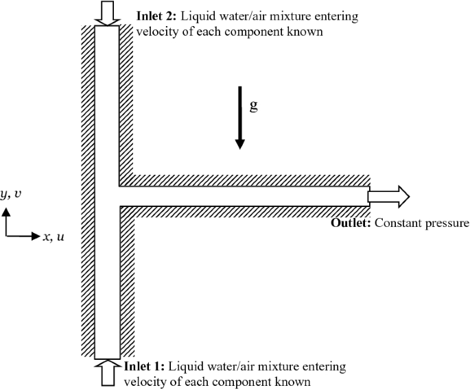
  Fig. P3.36

• 3.37. A parametric study on the effect of the inlet velocities and gas volume fraction from Problem 3.36 is needed. However, before performing this study using the homogeneous model , the inaccuracies of the model must first be quantified. The inaccuracies should be quantified by comparing the homogeneous results to a volume-averaged multifluid model. Therefore, set up the governing equation using a volume-averaged multifluid model with the corresponding boundary conditions with the same assumptions used in Problem 3.36.

• 3.38. Consider a case of annular flow in which the liquid flows as a film on the wall of a pipe while the gas flows down the central cylindrical core. For a pipe of diameter D, let the interfacial and wall shear stresses be $\tau_{\delta }$ and $\tau_{W}$ as given inputs, respectively. Assuming vertical cocurrent flow configuration as shown in Fig. P3.38, develop the formulation for one-dimensional, unsteady, laminar flow with multifluid modeling.

  

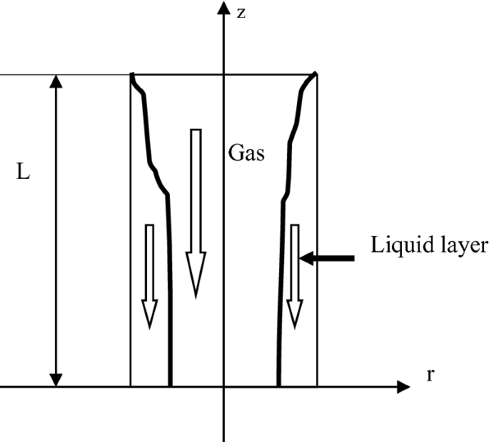
  Fig. P3.38

• 3.39. Deduce the general one-dimensional governing equations for mass and momentum for stratified turbulent flow of two phases (1) and (2) with evaporation over a flat plate as shown in Fig. P3.39.

  

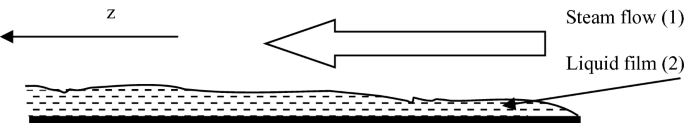
  Fig. P3.39

• 3.40. Formulate the analysis for heat transfer for Problem 3.39 using drift flux model. Assume steady, incompressible flow with negligible viscous dissipation . Use the results obtained in Problem 3.39 in carrying out the analysis.

• 3.41. Formulate steady flow in a one-dimensional nozzle under compressible inviscid conditions. The problem should be modeled as a homogeneous two-component flow with no phase change. Neglect the effects of surface tension . Obtain velocity and volume fraction distribution along the nozzle.

• 3.42. Derive the equations for mass, momentum, and energy for the flow of compressible gas through a channel containing dispersed particles. The flow occurs at high speed. Neglect the following effects: exchange of momentum, heat and mass with the channel walls, phase change, chemical reactions , viscous drag and viscous dissipation , and gravity. Assume the flow is one-dimensional, steady, and constant particle phase density. Do the analysis using the area-averaged multifluid models for channel flows.

• 3.43. For a coal classifier with $\varvec{L}_{\varvec{s}} = {\mathbf{1}}\,{\text{m}}$ and $\varvec{V}_{\varvec{s}} = {\mathbf{10}}\,{\text{m}}/{\text{s}}$, ${\mathbf{Sk}} = 0.04$ for particles with D = 30 microns, what is the ${\mathbf{Sk}}$ for particles with D = 300 microns? Is the mixture model appropriate for the larger diameter particles?

• 3.44. For a mineral processing system, $L_{\text{s}} = 0.2\,{\text{m}}$ and $V_{\text{S}} = 2\,{\text{m}}/{\text{s}}$, ${\text{Sk}} = 0.005$ for particles with D = 300 microns. Which multiphase model(s) is/are appropriate?

• 3.45. Saturated liquid water at 1 atm flows upward with a (uniform) velocity of 1 m/s $\left( {U_{\ell } = 1\,{\text{m}}/{\text{s}}} \right)$ between two parallel plates with a large distance in between. A heated vertical plate is inserted into the liquid, and film boiling occurs on both surfaces of the plate (see Fig. P3.45). For simplicity, we can assume that the liquid flow is not affected by the vapor motion and no slip condition is valid at the liquid–vapor interface (i.e., $u_{\text{v}} (\delta ) = U_{\ell } )$. Assuming that the convective terms in energy and momentum equations are negligible, the governing equations in the vapor film become:

  

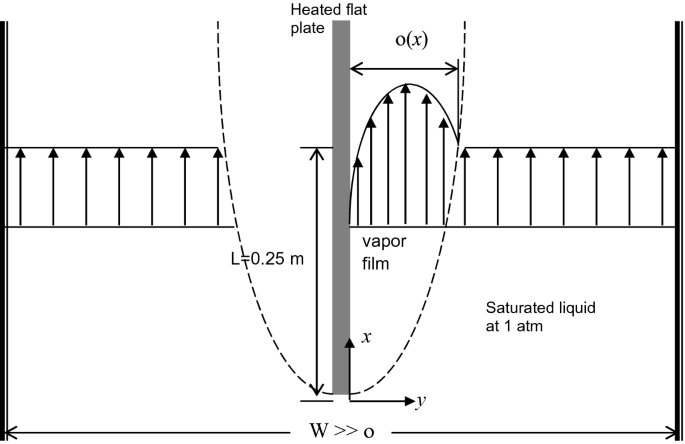
  Fig. P3.45

  $$ \mu_{\text{v}} \frac{{\partial^{2} u_{\text{v}} }}{{\partial y^{2} }} + g(\rho_{\text{v}} - \rho_{\ell } ) = 0,\quad\frac{{\partial^{2} T_{\text{v}} }}{{\partial y^{2} }} = 0 $$

  • (a) Determine the momentum and energy boundary conditions at the plate surface (y = 0), as well as the interfacial conditions at the liquid–vapor interface $(y=\delta (x))$.

  • (b) Determine the mass flow rate of vapor per unit width, $\Gamma(\delta)$ as a function of film thickness , $\delta$.

  • (c) Calculate the film thickness at 0.25 m from the bottom edge of the plate, if the heat flux applied by the flat plate is 1 kW/m² on each side.

  • (d) How would the film thickness change with increasing liquid velocity, $U_{\ell }$?

• 3.46. Saturated liquid water-gas mixture at 80 °C (353 K) flows through the manifold channels of a polymer electrolyte fuel cell (PEFC). The pressure of the manifold can be assumed constant at 100 kPa. The gas mixture contains water vapor, and the remainder is 80% nitrogen (N₂, MW_N2 = 32 gm/mol) and 20% oxygen (O₂, MW_O2 = 32 gm/mol) by weight.

  • a. Assuming ideal gas mixture, calculate the (intrinsic) density of the gas mixture. Saturation pressure of water at 80 °C is 47 kPa. MW_H2O = 18 gm/mol.

  • b. Intrinsic average velocity of gas mixture is 2 m/s. If the area fraction of liquid is $\varepsilon_{l} = 0.05$ and the quality of mixture is x = 0.75, calculate the intrinsic average velocity of the liquid phase.

  • c. If the manifold is of 1-mm square cross section, calculate the thickness of the film.

  • d. Assuming Boysan’s correlation for momentum exchange coefficient, $K_{jk}$ is applicable in the modified form below, calculate the interactive force $\left\langle {\varvec{F}_{jk} } \right\rangle$ between the liquid and vapor.

    $$ \begin{aligned} K_{jk} & = \frac{3}{4}f\frac{{\varepsilon_{j} \left\langle {\rho_{k} } \right\rangle^{k} }}{{\delta_{j} }}\left| {\left\langle {{\mathbf{V}}_{j} } \right\rangle^{j} - \left\langle {{\mathbf{V}}_{k} } \right\rangle^{k} } \right|, \quad f = \frac{24}{Re } \\ Re & = \frac{{\left\langle {\rho_{k} } \right\rangle^{k} \left| {\left\langle {{\mathbf{V}}_{j} } \right\rangle^{j} - \left\langle {{\mathbf{V}}_{k} } \right\rangle^{k} } \right|\delta_{j} }}{{\mu_{k} }},\quad \left\langle {{\mathbf{F}}_{jk} } \right\rangle = K_{jk} \left( {\left\langle {{\mathbf{V}}_{j} } \right\rangle^{j} - \left\langle {{\mathbf{V}}_{k} } \right\rangle^{k} } \right) \\ \mu_{\ell } & = 3.55 \times 10^{ - 6} \,\text{Pa}\,\text{s};\quad\mu_{\text{g}} = 2.15 \times 10^{ - 5} \,\text{Pa}\,\text{s} \\ \end{aligned} $$

• 3.47. Electroosmosis is flow induced by an external electric field. When surfaces acquire a finite charge density and are in contact with a polar solution, they induce a distribution of electrical charges within the electrically charged solution. Electroosmosis is used in biochip technology as a pumping mechanism in MEMS devices for chemical and biological analysis and diagnoses. Two-fluid electroosmotic flow is used in many microfluids. The working fluid needs to be a conducting liquid with significant electrical conductivity to function properly. As shown in Fig. P3.47, a high electroosmotic mobility liquid is at the bottom of the channel, and a low electroosmotic mobility liquid is in the upper section of the microchannel . When an electric field is applied across the channel, pressure and electroosmosis effects drive the liquids. The flow depends on the viscosity ratio of the two fluids, the external electric field, electroosmosis characteristics of the high mobility fluid, and the interfacial curvature between the two fluids. Develop the steady formulation for velocity and the electric potential due to an electrically applied field caused by charges on the wall.

  

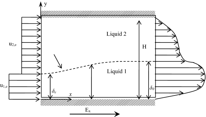
  Fig. P3.47

References

ANSYS fluent theory guide. (2017). ANSYS, Inc.
Avedisian, C. T. (1997). Soot formation in spherically symmetric droplet combustion. In I. Irvin Glassman, F. L. Dryer, & R. F. Sawyer (eds) Physical and chemical aspects of combustion (pp. 135–160). Gordon and Breach Publishers.
Avedisian, C. T. (2000). Recent advances in soot formation from spherical droplet flames at atmospheric pressure. Journal of Propulsion and Power, 16, 628–656.
Bejan, A. (2013). Convection heat transfer (4th ed.). New York: Wiley.
Bergman, T. L., & Lavine, A. S. (2017). Fundamentals of heat and mass transfer (8th ed.). New York: Wiley.
Boysan, F. (1990). A two-fluid model for fluent. Sheffield, England: Flow Simulation Consultants Ltd.
Edwards, D. K., Denny, V. E., & Mills, A. F. (1979). Transfer process. New York: Hemisphere.
Faghri, A. (2016). Heat pipe science and technology (2nd ed.). Columbia, MO: Global Digital Press.
Faghri, A., Zhang, Y., & Howell, J. R. (2010). Advanced heat and mass transfer. Columbia, MO: Global Digital Press.
Hewitt, G. F. (1998). “Multiphase fluid flow and pressure drop”, heat exchanger design handbook (Vol. 2). New York, NY: Begell House.
Hirschfelder, J. O., Curtiss, C. F., & Bird, R. B. (1966). Molecular theory of gases and liquids. New York: Wiley.
Kays, W. M., Crawford, M. E., & Weigand, B. (2004). Convective heat transfer (4th ed.). New York, NY: McGraw-Hill.
Kleijn, C. R. (1991). A mathematical model of the hydrodynamics and gas phase reaction in silicon LPCVD in a single wafer reactor. Journal of the Electrochemical Society, 138, 2190–2200.
Lock, G. S. H. (1994). Latent heat transfer. Oxford University, Oxford, UK: Oxford Science Publications.
Mahajan, R. L. (1996). Transport phenomena in chemical vapor-deposition systems. In Advances in heat transfer. Academic Press, San Diego, CA.
Manninen, M., Taivassalo, V., & Kallio, S. (1996). On the mixture model for multiphase flow. VTT Publications 288, Technical Research Centre of Finland.
Schiller, L., & Naumann, A. (1935). A drag coefficient correlation. Zeitschrift des Vereins Deutscher Ingenieure, 77, 318–320.
Welty, J. R., Rorrer, G. L., & Foster, D. G. (2014). Fundamentals of momentum, heat and mass transfer (6th ed.). New York, NY: Wiley.
White, F. M. (2005). Viscous fluid flow (3rd ed.). New York: McGraw-Hill.
Author information
Authors and Affiliations
Corresponding author