Counters in Kappa: Semantics, Simulation, and Static Analysis

Abstract

Site-graph rewriting languages, such as Kappa or BNGL, offer parsimonious ways to describe highly combinatorial systems of mechanistic interactions among proteins. These systems may be then simulated efficiently. Yet, the modeling mechanisms that involve counting (a number of phosphorylated sites for instance) require an exponential number of rules in Kappa. In BNGL, updating the set of the potential applications of rules in the current state of the system comes down to the sub-graph isomorphism problem (which is NP-complete).

In this paper, we extend Kappa to deal both parsimoniously and efficiently with counters. We propose a single push-out semantics for Kappa with counters. We show how to compile Kappa with counters into Kappa without counters (without requiring an exponential number of rules). We design a static analysis, based on affine relationships, to identify the meaning of counters and bound their ranges accordingly.

1 Introduction

Site-graph rewriting is a paradigm for modeling mechanistic interactions among proteins. In Kappa [18] and BNGL [3, 40], rewriting rules describe how instances of proteins may bind and unbind, and how each protein may activate the interaction sites of each others, by changing their properties. Sophisticated signaling cascades may be described. The long term behavior of such models usually emerges from competition against shared-resources, proteins with multiple-phosphorylation sites, scaffolds, separation of scales, and non-linear feedback loops.

It is often desirable to add more structure to states in order to describe generic mechanisms more compactly. In this paper, we consider extending Kappa with counters with numerical values. As opposed to the properties of classical Kappa sites, which offer no structure, counters allow for expressive preconditions (such as the value of a counter is less than 2), but also for generic update functions (such as incrementing or decrementing the current value of a counter by a given value independently of its current value). Without counters, such update functions would require one rule per potential value of the counter. This raises efficiency issues for the simulation and also blurs any potential reasoning on the causality of the system.

However adding counters cannot be done without consequences. The efficiency of Kappa simulations mainly relies on two ingredients. Firstly, Kappa graphs are rigid [16, 39]: an embedding from a connected site-graph into a site-graph, when it exists, is fully determined by the image of one node. Thanks to rigidity, searching for the occurrences of a sub-graph into another graph (up-to isomorphism) may be done without backtracking (once a first node has been placed), and embeddings can be described in memory very concisely. Secondly, the representation of the set of potential applications of rules relies on a categorical construction [6] that optimizes sharing among patterns. Yet this construction cannot cope with the more expressive patterns that involve counters. In order to efficiently simulate models with counters, we need an efficient encoding that preserves rigidity and that use classical site-graph patterns.

Fig. 1.

Three representations for the phosphorylation of a site. We assume that the rate of phosphorylation of a site in a protein in which exactly k sites are already phosphorylated, is equal to the value f(k). The function f is left as a parameter of the model. In (a), we do not use counters. In order to get the number of sites that are already phosphorylated, we have to document the state of all the sites of the protein. In this rule, there are exactly 2 sites already phosphorylated, thus the rate of the rule is equal to f(2). In (b), we use a counter to encode the number of sites already phosphorylated. The variable k, that is introduced by the notation @k, contains the number of sites that are phosphorylated before the application of the rule. Thus, the rate of the rule is equal to f(k). In the right hand side, the notation $+1$ indicates that the counter is incremented at each application of the rule. The rule in (b) summarizes exactly 8 rules of the kind of the one in (a) (it defines the phosphorylation of the site regardless of the states of the three other phosphorylation sites). In (c), we abstract away the sites and keep only the counter. The notation @k binds the variable k to the value of the counter. The left hand side also indicates that the rule may be applied only if the value of the counter is less than or equal to 3 (so that at least one site is not already phosphorylated). The right hand side specifies that the value of the counter is incremented at each application of the rule and that after the application of a rule, the value of the counter is always less than or equal to 4. The rule in (c) stands for 32 rules of the kind of the one in (a) (it depends neither on which site is phosphorylated, nor on the state of the three other sites).

Let us consider a case study so as to illustrate the need for counters in Kappa. This example is inspired from the behavior of the protein KaiC that is involved in the synchronization of the proteins in the circadian clock. We consider one kind of protein with n identified sites that can get phosphorylated. Indeed, n is equal to 6 in the protein KaiC. We take n equal to 4 to make graphical representation lighter. We will make n diverge towards the infinity so as to empirically estimate the combinatorial complexity of several encoding schemes.

The rate of phosphorylation/dephosphorylation of each site, depends on the number of sites that are already phosphorylated. In Fig. 1(a), we provide the example of a rule that phosphorylates the site of the protein, assuming that the sites and are already phosphorylated and that the site is not. Proteins are depicted as rectangles. Sites are depicted clockwise from the site to the site starting at the top left corner of the protein. Phosphorylation states are depicted with a black mark when the site is phosphorylated, and with a white mark otherwise. To fully encode this model in Kappa, we would require $n\cdot 2^{n}$ rules. Indeed, we need to decide whether this is a phosphorylation or a dephosphorylation (2 possibilities), then on which site to apply the transformation (n possibilities), then what the state of the other sites is ($2^{n-1}$ possibilities). This combinatorial complexity may be reduced by the means of counters. We consider a fresh site (this site is depicted on the right of the protein) and we assume that this site takes numerical values. Writing each rule carefully, we can enforce that the value of this site is always equal to the number of the sites that are phosphorylated in the protein instance. Thanks to this invariant, describing our model requires $2{\cdot }n$ rules according to whether we describe a phosphorylation or a dephosphorylation (2 possibilities) and to which site the transformation is applied (n possibilities). An example of rule for the phosphorylation of the site is given in Fig. 1(b). The notation @k assigns the value of the counter before the application of the rule to the variable k. Then the rate of the rule may depend on the value of k. This way, we can make the rate of phosphorylation depend on the number of sites already phosphorylated in the protein. Since there are only n sites that may be phosphorylated, it is straightforward to see that the counter may range only between the values 0 and n.

If only the number of phosphorylated sites matters, we can go even further: we need just one counter and two rules, one for phosphorylating a new site (e. g. see Fig. 1(c)) and one for dephosphorylating it. The value of the counter is no longer related explicitly to a number of phosphorylated sites, thus we need another way to specify that the value of the counter is bounded. We do this, by specifying in the precondition of the rule that the phosphorylation rule may be applied only if the value of the counter is less or equal to $n-1$, which entails that the value of the counter may range only between the values 0 and n.

Not only parsimonious description of the mechanistic interactions in a model eases the process of writing a model, enhances readability and leads to more efficient simulation, but also it may provide better grain of observation of the system behavior. In Fig. 2, we illustrate this by looking at three causal traces that denote the same execution, but for three different encodings. Intuitively, causal traces [14, 15] are inspired by event structures [43]. They describe sets of traces seen up to permutation of concurrent computation steps. The level of representation for the potential configurations of each protein impacts the way causality is defined, because what is tested in rules depends on the representation level. In our case study, the phosphorylation of each site is intuitively causally independent: one site may be phosphorylated whatever the state of the other sites is. Without counters, the only way to specify that the rate of phosphorylation depends on the number of the sites that are already phosphorylated, is to detail the state of every site of the protein in the precondition of the rule. This induces spurious causal relations (e. g. see Fig. 2(a)). Utilizing counters relaxes this constraint. However it is important to equip counters with arithmetic. Without arithmetic, a rule may only set the value of a counter to a constant value. Thus for implementing counter increment, rules have to enumerate the potential values of the counter before their applications, and set the value of this counter accordingly. This induces again spurious causal relations (e. g. see Fig. 2(b)). With arithmetic, incrementing counters becomes a generic operation that may be applied independently of the current value of the counter. As a result the phosphorylation of the four sites can be seen as causally independent (e. g. see Fig. 2(c)). This faithfully represents the fact that the phosphorylation of the four sites may happen in arbitrary order.

Fig. 2.

Three causal traces. Each causal trace is made of a set of partially ordered computation steps. Roughly speaking, a computation step precedes another one, if the former is necessary to perform the later. Each computation step is denoted as an arrow labeled with the rule that implements it. In (a), counters are not used. Every rule tests the full configuration of the protein. At this level of representation, the k-th phosphorylation causally precedes the $k+1$-th one, whatever the order in which the sites have been phosphorylated. In (b), an additional site is used to record the number of phosphorylated sites in its internal state. With this encoding, the number of phosphorylated sites cannot be incremented without testing explicitly the internal state of the additional site. As a consequence, here again, at this level of representation, each phosphorylation causally depends on the previous one. In (c), we use the expressiveness of arithmetic. We use generic rules to increment the counter regardless of its current value. Hence, at this level of representation, the phosphorylation of the four sites become independent, which flatten the causal trace.

Contribution. Now we describe the main contributions of this paper.

In Sect. 2, we formalize a single push-out (SPO) semantics for Kappa with counters. Having a categorical framework dealing with counters, as opposed to implementing counters as syntactic sugar, is important. Firstly, this semantics will serve as a reference for the formal specification of the behavior of counters. Secondly, the categorical setting of Kappa provides efficient ways to define causality [14, 15], symmetries [25], and some sound symbolic reasonings on the behavior of the number of occurrences of patterns [1, 26] that are used in model reduction. Including counters in the categorical semantics of Kappa allows for extending the definition of these concepts to Kappa with counters for free.

Yet different encodings of counters may be necessary to extend other tools for Kappa. In Sect. 3, we propose a couple of translations from Kappa with counters into Kappa without counters. The goal is to simulate models with counters efficiently without modifying the implementation of the Kappa simulator, KaSim [17]. The first encoding requires counters to be bounded from below and it supports only two kinds of preconditions over counters: a rule may require the value of a counter to be equal to a given value, or to be greater than a given value. Requiring the value of a counter to be less than a given value is not supported. The second encoding supports equality and inequality (in both directions) tests. But it requires the value of each counter to be bounded also from above.

Static analysis is needed not only to prove these requirements, but also to retrieve the meaning of counters. In Sect. 4, we introduce a generic abstract interpretation framework [9] to infer the properties of reachable states of a model. This framework is parametric with respect to a class of properties. In Sect. 5, we instantiate this framework with a relational numerical analysis aiming at relating the value of each counter to its interpretation with respect to the state of the other sites. This is used to detect and prove bounds on the range of counters.

Related Works. Many modeling languages support arbitrary data-types. In Spatial-Kappa [41], counters encode the discrete position of agents. More generally, in Chromar [29] and in colored Petri nets [30, 35], agents may be tagged with values in arbitrary auxiliary programming languages. In ML-Rules [28], agents with attributes continuously diffuse within compartments and collide to interact.

We have different motivations. Our goal is to enrich the state of proteins with some redundant information, so as to reduce the number of rules that are necessary to describe their mechanistic interactions. Also we want to avoid too expressive data-types, which could not be integrated within simulation, causality analysis, and static analysis tools, without altering their performance. For instance, analysis of colored Petri nets usually relies on unfolding them into classical ones. Unfolding rule sets into classical ones does not scale because the number of rules would become intractable. Thus we need tools which deal directly with counters.

An encoding of two-counter machines has been proposed to show that most problems in Kappa are undecidable [19, 34]. We represent counters the same way in our first encoding, but we provide atomic implementation for more primitives.

The number of isomorphic classes of connected components that may occur in Kappa models during simulation is usually huge (if not infinite), which prevents from using agent-centric approaches [4]. For instance, one of the first non-toy model written in Kappa was involving more than $10^{19}$ kinds of bio-molecular complexes [16, 26]. Kappa follows a rule-centric approach which allows for the description and the execution of models independently from the number of potential complexes. Also, Kappa disallows to describe diffusion of molecules. Instead the state of the system is assumed to satisfy the well-mixed assumption. This provides efficient ways to represent and update the distribution of potential computation steps, along a simulation [6, 17].

Equivalent sites [3] or hyperlinks [31] offer promising solutions to extend the decision procedures to extract minimal causal traces in the case of counters, but the rigidity of graphs is lost. Our encodings rely neither on the use of equivalent sites, nor on expanding the rules into more refined and more numerous ones. Hence our encodings preserve the efficiency of the simulation.

Our analysis is based on the use of affine relationships [32]. It relates counter values to the state of the other variables. Such relationships look like the ones that help understanding and proving the correctness of semaphores [20, 21]. We use the decision procedure that is described in [23, 24] to deduce bounds on the values of counters from the affine relationships. The cost of each atomic computation is cubic with respect to the number of variables. Abstract multi-sets [27, 38] may succeed in expressing the properties of interest, but they require a parameter setting a bound on the values that can abstract precisely. In practice, their time-cost is exponential as soon as this bound is not chosen big enough. Our abstraction has an infinite height. It uses widening [11] and reduction [12] to discover the bounds of interest automatically. Octagons [36, 37] have a cubic complexity, but they cannot express the properties involving more than two variables which are required in our context. Polyhedra [13] express all the properties needed for an exponential time-cost in practice.

2 Kappa

In this section, we enrich the syntax and the operational semantics of Kappa so as to cope with counters. We focus on the single push-out (SPO) semantics.

2.1 Signature

Firstly we define the signature of a model.

Definition 1

(signature). The signature of a model is defined as a tuple $\varSigma =(\varSigma _{\textit{ag}},\varSigma _{\textit{site}},\varSigma _{\textit{int}},\varSigma ^{\textit{int}}_{\textit{ag-st}},\varSigma ^{\textit{lnk}}_{\textit{ag-st}},\varSigma ^{\$}_{\textit{ag-st}},\textit{Prop}_{\$},\textit{Update}_{\$})$ where:

• 1. $\varSigma _{\textit{ag}}$ is a finite set of agent types,

• 2. $\varSigma _{\textit{site}}$ is a finite set of site identifiers,

• 3. $\varSigma _{\textit{int}}$ is a finite set of internal state identifiers,

• 4. $\varSigma ^{\textit{lnk}}_{\textit{ag-st}}$, $\varSigma ^{\textit{int}}_{\textit{ag-st}}$, and $\varSigma ^{\$}_{\textit{ag-st}}$ are three site maps (from $\varSigma _{\textit{ag}}$ into $\wp (\varSigma _{\textit{site}})$)

• 5. $\textit{Prop}_{\$}$ is a potentially infinite set of non-empty subsets of $\mathbb {Z}$,

• 6. $\textit{Update}_{\$}$ is a potentially infinite set of functions from $\mathbb {Z}$ to $\mathbb {Z}$ containing the identity function.

For every $G\in \textit{Prop}_{\$}$, we assume that for every function $f\in \textit{Update}_{\$}$, the set $\{f(k)\;|\;k\in G\}$ belongs to the set $\textit{Prop}_{\$}$, and that for every element $k\in G$, the set $\{k\}$ belongs to the set $\textit{Prop}_{\$}$ as well.

Agent types in $\varSigma _{\textit{ag}}$ denote the agents of interest, the different kinds of proteins for instance. A site identifier in $\varSigma _{\textit{site}}$ represents an identified locus for a capability of interaction. Each agent type $\textit{A} \in \varSigma _{\textit{ag}}$ is associated with a set of sites $\varSigma ^{\textit{int}}_{\textit{ag-st}}(\textit{A} )$ with an internal state (i.e. a property), a set of sites $\varSigma ^{\textit{lnk}}_{\textit{ag-st}}(\textit{A} )$ which may be linked, and a set of sites $\varSigma ^{\$}_{\textit{ag-st}}(\textit{A} )$ with a counter. We assume without any loss of generality that the three sets $\varSigma ^{\textit{lnk}}_{\textit{ag-st}}(\textit{A} )$, $\varSigma ^{\textit{int}}_{\textit{ag-st}}(\textit{A} )$, and $\varSigma ^{\$}_{\textit{ag-st}}(\textit{A} )$ are disjoint pairwise. The set $\textit{Prop}_{\$}$ contains the set of valid conditions that may be checked on the value of counters, whereas the set $\textit{Update}_{\$}$ contains all the possible update functions for the value of counters. We assume that every singleton that is included in a valid condition is a valid condition as well. In this way, a valid condition may be refined to a fully specified value. Additionally, the image of a valid condition is required to be valid, so that the post-condition obtained by applying an update function to a valid precondition, is valid as well.

Example 1

(running example). We define the signature for our case study as the tuple $(\varSigma _{\textit{ag}},\varSigma _{\textit{site}},\varSigma _{\textit{int}},\varSigma ^{\textit{int}}_{\textit{ag-st}},\varSigma ^{\textit{lnk}}_{\textit{ag-st}},\varSigma ^{\$}_{\textit{ag-st}},\textit{Prop}_{\$},\textit{Update}_{\$})$ where:

• 1. $\varSigma _{\textit{ag}}:=\{{\textit{P} }\}$;

• 2. ;

• 3. $\varSigma _{\textit{int}}:=\{\circ ,\bullet \}$;

• 4. ;

• 5. ;

• 6. ;

• 7. $\textit{Prop}_{\$}$ is the set of all the convex parts of $\mathbb {Z}$;

• 8. $\textit{Update}_{\$}$ contains the function mapping each integer $n\in \mathbb {Z}$ to its successor, and the function mapping each integer $n\in \mathbb {Z}$ to its predecessor.

The agent type P denotes the only kind of proteins. It has four sites , , , carrying an internal state and one site carrying a counter.   $\square$

Until the rest of the paper, we assume given a signature $\varSigma$.

Fig. 3.

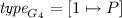
Four site-graphs $G_1$, $G_2$, $G_3$, and $G_4$.

2.2 Site-Graphs

Site-graphs describe both patterns and chemical mixtures. Their nodes are typed agents with some sites which may carry internal and binding states, and counters.

Definition 2

(site-graph). A site-graph is a tuple $G=(\mathcal {A}_{},\textit{type}_{},\mathcal {S}_{},\mathcal {L}_{},p\kappa _{},c\kappa _{})$ where:

• 1. $\mathcal {A}_{}$ is a finite set of agents,

• 2. $\textit{type}_{}\;:\;\mathcal {A}_{}\rightarrow \varSigma _{\textit{ag}}$ is a function mapping each agent to its type,

• 3. $\mathcal {S}_{}$ is a set of sites satisfying the following property:

  $$\mathcal {S}_{}\subseteq \{(n,i)\;|\; n\in \mathcal {A}_{}, i\in \varSigma _{\textit{ag-st}}(\textit{type}_{}(n))\}{\textit{,}}$$

• 4. $\mathcal {L}_{}$ maps the set:

  $$\{(n,i)\in \mathcal {S}_{}\;|\;i\in \varSigma ^{\textit{lnk}}_{\textit{ag-st}}(\textit{type}_{}(n))\}$$

  to the set:

  $$\{(n,i)\in \mathcal {S}_{}\;|\;i\in \varSigma ^{\textit{lnk}}_{\textit{ag-st}}(\textit{type}_{}(n))\}\cup \{\dashv ,-\}{\textit{,}}$$

  such that:

  • (a) for any site $(n,i)\in \mathcal {S}_{}$, we have $\mathcal {L}_{}(n,i)\ne (n,i)$;

  • (b) for any two sites $(n,i),(n',i')\in \mathcal {S}_{}$, we have $(n',i')=\mathcal {L}_{}(n,i)$ if and only if $(n,i)=\mathcal {L}_{}(n',i')$;

• 5. $p\kappa _{}$ maps the set $\{(n,i)\in \mathcal {S}_{}\;|\;i\in \varSigma ^{\textit{int}}_{\textit{ag-st}}(\textit{type}_{}(n))\}$ to the set $\varSigma _{\textit{int}}$;

• 6. $c\kappa _{}$ maps the set $\{(n,i)\in \mathcal {S}_{}\;|\;i\in \varSigma ^{\$}_{\textit{ag-st}}(\textit{type}_{}(n))\}$ to the set $\textit{Prop}_{\$}$.

For a site-graph $G$, we write as $\mathcal {A}_{G}$ its set of agents, $\textit{type}_{G}$ its typing function, $\mathcal {S}_{G}$ its set of sites, and $\mathcal {L}_{G}$ its set of links. Given a site-graph $G$, we write as $\mathcal {S}^{\textit{lnk}}_{G}$ (resp. $\mathcal {S}^{\textit{int}}_{G}$, resp. $\mathcal {S}^{\$}_{G}$) its set of binding sites (resp. property sites, resp. counters) that is to say the set of the sites (n, i) such that $i\in \varSigma ^{\textit{lnk}}_{\textit{ag-st}}(\textit{type}_{G}(n))$ (resp. $i\in \varSigma ^{\textit{int}}_{\textit{ag-st}}(\textit{type}_{G}(n))$, resp. $i\in \varSigma ^{\$}_{\textit{ag-st}}(\textit{type}_{G}(n))$).

Let us consider a binding site $(n,i)\in \mathcal {S}^{\textit{lnk}}_{G}$. Whenever $\mathcal {L}_{G}(n,i)=\dashv$, the site (n, i) is free. Various levels of information may be given about the sites that are bound. Whenever $\mathcal {L}_{G}(n,i)=-$, the site (n, i) is bound to an unspecified site. Whenever $\mathcal {L}_{G}(n,i)=(n',i')$ (and hence $\mathcal {L}_{G}(n',i')=(n,i)$), the sites (n, i) and $(n',i')$ are bound together.

A chemical mixture is a site-graph in which the state of each site is fully specified. Formally, a site-graph $G$ is a chemical mixture, if and only if, the three following properties:

• 1. the set $\mathcal {S}_{G}$ is equal to the set $\{(n,i)\;|\;n\in \mathcal {A}_{G},\;i\in \varSigma _{\textit{ag-st}}(\textit{type}_{G}(n))\}$;

• 2. every binding site is free or bound to another binding site (i. e. for every $(n,i)\in \mathcal {S}_{G}\cap \varSigma ^{\textit{lnk}}_{\textit{ag-st}}(\textit{type}_{G}(n))$, $\mathcal {L}_{G}(n,i)\ne -$);

• 3. every counter has a single value (i. e. for every $(n,i)\in \varSigma ^{\$}_{\textit{ag-st}}$, $c\kappa _{G}(n,i)$ is a singleton);

are satisfied.

Example 2

(running example). In Fig. 3, we give a graphical representation of the four site-graphs, $G_1$, $G_2$, $G_3$, and $G_4$ that are defined as follows:

• 1.

  • (a) $\mathcal {A}_{G_1}=\{1\}$,

  • (b) ,

  • (c) ,

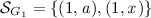  • (d) $\mathcal {L}_{G_1}=\emptyset$,

  • (e) $p\kappa _{G_1}=[(1,a) \mapsto \circ ]$,

  • (f) $c\kappa _{G_1}=[(1,x) \mapsto \{k\in \mathbb {Z}\;|\;k \le 2\}]$;

• 2.

  • (a) $\mathcal {A}_{G_2}=\{1\}$,

  • (b) ,

  • (c) ,

  • (d) $\mathcal {L}_{G_2}=\emptyset$,

  • (e) $p\kappa _{G_2}=[]$,

  • (f) $c\kappa _{G_2}=[(1,x) \mapsto \{k\in \mathbb {Z}\;|\;k \le 2\}]$;

• 3.

  • (a) $\mathcal {A}_{G_3}=\{1\}$,

  • (b) ,

  • (c) ,

  • (d) $\mathcal {L}_{G_3}=\emptyset$,

  • (e) $p\kappa _{G_3}=[(1,a) \mapsto \bullet ]$,

  • (f) $c\kappa _{G_3}=[(1,x) \mapsto \{k\in \mathbb {Z}\;|\;k \le 3\}]$;

• 4.

  • (a) $\mathcal {A}_{G_4}=\{1\}$,

  • (b) ,

  • (c) ,

  • (d) $\mathcal {L}_{G_4}=\emptyset$,

  • (e) $p\kappa _{G_4}=[(1,a) \mapsto \circ , (1,b) \mapsto \bullet , (1,c) \mapsto \bullet , (1,d) \mapsto \circ ]$,

  • (f) $c\kappa _{G_4}=[(1,x) \mapsto \{2\}]$;

The white site on the side of proteins is always the site . The other sites, starting from the top-left one denote the sites , , , and clockwise.   $\square$

2.3 Sliding Embeddings

In classical Kappa, two site-graphs may be related by structure-preserving injections, which are called embeddings. Here, we extend their definition to cope with counters. There are two main issues: a rule may require the value of a given counter to belong to a non-singleton set; also updating counters may involve arithmetic computations. The smaller the set of the potential values for a counter is, the more information we have. Thus, embeddings may map the potential values of a given counter into a subset. In order to cope with update functions, we equip embeddings with some arithmetic functions which explain how to get from the value of the counter in the source of the embedding to its value in the target. This way, our embeddings not only define instances of site-graphs, but they also contain the information to compute the values of counters.

Fig. 4.

Three sliding embeddings from the $G_2$ respectively into the site-graphs $G_3$, $G_1$, and $G_4$. Only the second and the third embeddings are pure.

Definition 3

(sliding embedding). A sliding embedding from a site-graph G into a site-graph H is a pair $(h_e, h_{\$})$ where $h_e$ is a function of agents $h_e\;:\;\mathcal {A}_{G}\rightarrow \mathcal {A}_{H}$ and $h_{\$}$ is a function mapping the counters of the site-graph G to update functions $h_{\$}\;:\;\mathcal {S}^{\$}_{G} \rightarrow \textit{Update}_{\$}$ such that for all agent identifiers m, n, $n'\in \mathcal {A}_{G}$ and for all site identifiers $i\in \varSigma _{\textit{ag-st}}(\textit{type}_{G}(n))$, $i'\in \varSigma _{\textit{ag-st}}(\textit{type}_{G}(n'))$, the following properties are satisfied:

• 1. if $m\ne n$, then $h_e(m)\ne h_e(n)$;

• 2. $\textit{type}_{G}(n) = \textit{type}_{H}(h_e(n))$;

• 3. if $(n,i)\in \mathcal {S}_{G}$, then $(h_e(n), i)\in \mathcal {S}_{H}$;

• 4. if $(n,i)\in \mathcal {S}^{\textit{lnk}}_{G}$ and $\mathcal {L}_{G}(n,i)=(n',i')$, then $\mathcal {L}_{H}(h_e(n),i)=(h_e(n'),i')$;

• 5. if $(n,i)\in \mathcal {S}^{\textit{lnk}}_{G}$ and $\mathcal {L}_{G}(n,i)=\dashv$, then $\mathcal {L}_{H}(h_e(n),i)=\dashv$;

• 6. if $(n,i)\in \mathcal {S}^{\textit{lnk}}_{G}$ and $\mathcal {L}_{G}(n,i)=-$, then $\mathcal {L}_{H}(h_e(n),i)\in \{-\}\cup \mathcal {S}_{H}$;

• 7. if $(n,i)\in \mathcal {S}^{\textit{int}}_{G}$ and $p\kappa _{G}(n,i)=\iota$, then $p\kappa _{H}(h_e(n),i)=\iota$;

• 8. if $(n,i)\in \mathcal {S}^{\$}_{G}$, then $c\kappa _{H}(h(n),i)\subseteq \{h_{\$}(k) \;|\;k\in c\kappa _{G}(n,i)\}$.

Two sliding embeddings between site-graphs, from E to F, and from F to G respectively, compose to form a sliding embedding from E to G (functions compose pair-wise). A sliding embedding $(h_e,h_{\$})$ such that $h_{\$}$ maps each counter to the identity function is called a pure embedding. A pure embedding from E to F is denoted as . Pure embeddings compose. Two site-graphs E and F are isomorphic if and only if there exist a pure embedding from E to F and a pure embedding from F to E. A pure embedding between two isomorphic site-graphs is called an isomorphism. When it exists, the unique pure embedding $(h_e,h_{\$})$ from a site-graph E into the site-graph F such that $\mathcal {A}_{E}\subseteq \mathcal {A}_{F}$ and $h_e(n)=n$ for every agent $n\in \mathcal {A}_{E}$, is called the inclusion from E to F and is denoted as $i_{E,F}$ or as . In such a case, we say that the site-graph E is included in the site-graph F. The inclusion from a site-graph into itself always exists and is called an identity embedding.

Example 3

(running example). We show in Fig. 4 three sliding embeddings from the site-graph $G_2$ respectively into the site-graphs $G_3$, $G_1$, and $G_4$. The first of these three sliding embeddings is assumed to increment the value of the counter of the site . The last two embeddings are pure.   $\square$

Let L, R, and D be three site-graphs, such that R is included in D, and let $\phi$ be a sliding embedding from L into D. Then there exist a site graph $D'$ that is included in L and a sliding embedding $\psi$ from $D'$ to R such that $i_{R,D}\psi = {\phi }i_{D',L}$ and such that $D'$ is maximal (w.r.t. inclusion among site-graphs) for this property. The pair $(D',i_{D',L},\psi )$ is called the pull-pack of the pair $(\phi ,i_{R,D})$.

Let L, R, and D be three site-graphs such that D is included in L. A partial sliding embedding from L into R is defined as a pair made of the inclusion $i_{D,L}$ and a sliding embedding from D to R. Sliding embeddings may be considered as partial sliding embeddings with the inclusion as the identity embedding. Partial sliding embeddings compose by the means of a pull-back (e.g. see Fig. 5(b)).

Fig. 5.

Composition of partial sliding embeddings.

Fig. 6.

Rule application.

2.4 Rules

Rules represent transformations between site-graphs. For the sake of simplicity, we only use a fragment of Kappa (we assume here that there are no side effects). Rules may break and create bonds between pairs of sites, change the properties of sites, update the value of counters. They may also create and remove agents. When an agent is created, all its sites must be fully specified: binding sites may be either free, or bound to a specific site, and the value of counters must be singletons. So as to ensure that there is no side-effect when an agent is removed, we also assume that the binding sites of removed agents are fully specified. These requirements are formalized as follows:

Definition 4

(rule). A rule is a partial sliding embedding such that:

• 1. (modified agents) for all agents $n\in \mathcal {A}_{D}$ such that $h_e(n)\in \mathcal {A}_{R}$ and for every site identifier $i\in \varSigma _{\textit{site}}(\textit{type}_{L}(n))$,

  • (a) the site (n, i) belongs to the set $\mathcal {S}_{L}$ if and only if $(h_e(n),i)$ belongs to set $\mathcal {S}_{R}$;

  • (b) if the site (n, i) belongs to the set $\mathcal {S}^{\textit{lnk}}_{L}$, then either $\mathcal {L}_{L}(n,i)=-$ and $\mathcal {L}_{R}(h_e(n),i)=-$, or $\mathcal {L}_{L}(n,i)\in \mathcal {S}^{\textit{lnk}}_{L}\cup \{\dashv \}$ and $\mathcal {L}_{R}(h_e(n),i)\in \mathcal {S}^{\textit{lnk}}_{R}\cup \{\dashv \}$;

  • (c) if the site (n, i) belongs to the set $\mathcal {S}^{\$}_{L}$, then the sets $c\kappa _{R}(h_e(n),i)$ and $\{h_{\$}(v)\;|\;v\in c\kappa _{L}(n,i)\}$ are equal.

• 2. (removed agents) for all agents $n\in \mathcal {A}_{L}$ such that $n\not \in \mathcal {A}_{D}$, for every site identifier $i\in \varSigma ^{\textit{lnk}}_{\textit{ag-st}}(\textit{type}_{L}(n))$, $(n,i)\in \mathcal {S}^{\textit{lnk}}_{L}$ and $\mathcal {L}_{L}(n,i)\in \mathcal {S}^{\textit{lnk}}_{L}\cup \{\dashv \}$.

• 3. (created agents) for all agents $n\in \mathcal {A}_{R}$ for which there exists no $n'\in \mathcal {A}_{D}$ such that $n=h_e(n')$, and for every site identifier $i\in \varSigma _{\textit{site}}(\textit{type}_{R}(n))$,

  • (a) the site (n, i) belongs to the set $\mathcal {S}_{R}$;

  • (b) if the site (n, i) belongs to the set $\mathcal {S}^{\textit{lnk}}_{R}$, then the binding state $\mathcal {L}_{R}(n,i)$ belong to the set $\mathcal {S}^{\textit{lnk}}_{R}\cup \{\dashv \}$;

  • (c) if the site (n, i) belongs to the set $\mathcal {S}^{\$}_{R}$, then $c\kappa _{R}(n,i)$ is a singleton.

In Definition 4, each agent that is modified occurs on both hand sides of a rule. Constraint 1a ensures that they document the same sites. Constraint 1b ensures that, if the binding state of a site is modified, then it has to be fully specified (either free, or bound to a specific site) in both hand sides of the rule. Constraint 1c ensures that the post-condition associated to a counter is the direct image of its precondition by its update function. Constraint 2 ensures that the agents that are removed have their binding sites fully specified. Constraint 3a ensures that, in the agents that are created, all the sites are documented. Beside, constraint 3b requires that the state of their binding site is either free or bound to a specific site. Constraint 3c ensures that their counters have a single value.

An example of a rule is given in Fig. 6(a).

A rule is usually denoted as (leaving the common region and the sliding embedding implicit). Rules are applied to site-graphs via pure embeddings using the single push-out construction [22].

Definition 5

(rule application [14]). Let r be a rule , $L'$ be a site-graph, and $h_L$ be a pure embedding from L to $L'$. Then, there exists a rule and a pure embedding such that the following properties are satisfied (e. g. see Fig. 6(c)):

• 1. $h_Rr = r'h_L$;

• 2. for all rules $r''$ between the site-graph $L'$ and a site-graph $R''$ and all embeddings $h'_R$ from R into $R''$ such that $h'_Rr = r''h_L$, there exists a unique pure embedding h from $R'$ into $R''$ such that $r''=hr'$ and $h'_R=hh_R$.

Moreover, whenever the site-graph $L'$ is a chemical mixture, the site-graph $R'$ is a chemical mixture as well.

We write $L' \xrightarrow {r} R'$ for a transition from the state $L'$ into the state $R'$ via an application of a rule r. Usually transition labels also mention the pure embedding ($h_L$ here), but we omit it since we do not use it in the rest of the paper.

Example 4

(running example). An example of rule application is depicted in Fig. 6. We consider the rule r that takes a protein with the site unphosphorylated and a counter with a value at least equal to 2, and that phosphorylates the site while incrementing the counter by 1 (e. g. see Fig. 6(a)). Note that the update function of the counter is written next to its post-condition in the right hand side of the rule. We apply the rule to a protein with the sites and phosphorylated, the site unphosphorylated, and the counter equal to 2 (e. g. see Fig. 6(b)). The result is a protein with the sites , , and phosphorylated, the site unphosphorylated and the counter equal to 3 (e. g. see Fig. 6(d)).   $\square$

A model $\mathcal {M}$ over a given signature $\varSigma$ is defined as the pair $(G_0,\mathcal {R})$ where $G_0$ is a chemical mixture, representing the initial state, and $\mathcal {R}$ is a set of rules. Each rule is associated with a functional rate which maps each potential tuple of values for the counters of the left hand side of the rule to a non negative real number. We write $\mathcal {C}(\mathcal {M})$ for the set of states obtained from $G_0$ by applying a potentially empty sequence of rules in $\mathcal {R}$.

3 Encoding Counters

In this section, we introduce two encodings from Kappa with counters into Kappa without counters. As explained in Sect. 1, our goal is to preserve the rigidity of site-graphs and to avoid the blow-up of the number of rules in the target model. This is mandatory to preserve the good performances of the Kappa simulator. Both encodings rely on syntactic restrictions over the preconditions and the update functions that may be applied to counters and on semantics ones about the potential range of counters. In Sects. 4 and 5, we provide a static analysis to check whether, or not, these semantics assumptions hold.

3.1 Encoding the Value of Counters as Unbounded Chains of Agents

In this encoding, each counter is bound to a chain of fictitious agents the length of which minus 1 denotes the value of the counter (another encoding not requiring the subtraction is possible but it would require side-effects). Encoding counters as chains of agents has already been used in the implementation of two-counter machines in Kappa [19, 34]. We slightly extend these works to implement more atomic operations over counters. We assume that the value of counters is bounded from below. For the sake of simplicity, we assume that counters range in $\mathbb {N}$, but arbitrary lower bounds may be considered by shifting each value accordingly. We denote by $\varOmega _{1}$ the set of the site-graphs that have a counter with a negative value. They are considered as erroneous states, since they may not be encoded with chains of agents.

Fig. 7.

Encoding the value of counters as unbounded chains of agents.

Only two kinds of guards are handled. A rule may require the value of a counter to be equal to a given number or that the value of a counter is greater than a given number. Rules testing whether a value is less than a given number require unfolding each such rule into several ones (one per potential value). Also when the rate of a rule depends on the value of some counters, we unfold each rule according to the value of these counters, so that the rate of each unfolded rule is a constant (the Kappa simulator requires all the instances of a given rule in a given simulation state to have the same rate, for efficiency concerns). For update functions, we only consider constant functions and the functions that increase/decrease the value of counters by a fixed value. Testing whether the value of a counter is equal to (resp. greater than) n, can be done by requiring the corresponding chain to contain exactly (resp. at least) $n+1$ agents (e. g. see Figs. 7(b) and (c)). Incrementing (resp. decrementing) the value of a counter is modeled by inserting (resp. removing) agents at the beginning its chain (e. g. see Fig. 7(d), resp. Fig. 7(e)). Setting a counter to a fixed value, requires to detach its full chain in order to create a new one of the appropriate length (e. g. see Fig. 7(f)). In such a case, the former chain remains as a junk. Thus the state of the model must be understood up to insertion of junk agents. We introduce the function $\textit{gc}_{1}$ that removes every chain of spurious agents not bound to any counter. We denote as (resp. ) the encoding of a site-graph G (resp. of a rule r).

3.2 Encoding the Value of Counters as Circular Lists of Agents

In this second encoding, each counter is bound to a ring of agents. Each such agent has three binding sites , , and , and a property site which may be activated, or not. In a ring, agents are connected circularly through their site and . Exactly one agent per ring is bound to a counter and exactly one agent per ring has the site activated. The value of the counter is encoded by the distance between the agent bound to the counter and the agent that is activated, scanning the agents by following the direction given by the site of each agent (clock-wisely in the graphical representation). We have to consider that counter values are bounded from above and below. Without any loss of generality, we assume that the length of each ring is the same, that is to say that counters range from 0 to $n-1$, for a given $n\in \mathbb {N}$. We denote by $\varOmega _{2}$ the set of the site-graphs with at least one counter not satisfying these bounds.

Fig. 8.

Encoding the value of counters as circular lists of agents.

Compared to the first encoding, this one may additionally cope with testing that a counter has a value less than a given constant without having to unfold the rule. Both encodings may deal with the same update functions. Testing whether a counter is equal to a value is done by requiring that the activated agent is at the appropriate distance of the agent that is connected to the counter (e. g. see Fig. 8(b)). It is worth noting that the intermediary agents are required to be not activated. This is not mandatory for the soundness of the encoding, this is an optimization that helps the simulator for detecting early that no embedding may associate a given agent of the left hand side of a rule to a given agent in the current state of the system. Inequalities are handled by checking that enough agents starting from the one that is connected to the counter and in the direction specified by the direction of the inequality, are not activated (e. g. see Fig. 8(c)). Incrementing/decrementing the value of a counter is modeled by making counter glide along the ring (e. g. see Figs. 8(d) and (e)). Special care has to be taken to ensure that the activated agent never crosses the agent linked to the counter (which would cause a numerical wrap-around). Assigning a given value to a counter requires to entirely remove the ring and to replace it with a fresh one (e. g. see Fig. 8(f)). It may be efficiently implemented without memory allocation. As in the first encoding, when the rate of a rule depends on the value of some counters, we unfold each rule according to the value of these counters, so that the rate of each unfolded rule is constant.

We introduce the function $\textit{gc}_{2}$ as the identity function over site-graphs (there are no junk agent in this encoding). We denote as (resp. ) the encoding without counter of a site-graph G (resp. of a rule r).

3.3 Correspondence

The following theorem states that, whenever there is no numerical overflow and providing that junk agents are neglected, the semantics of Kappa with counters and the semantics of their encodings are in bisimulation.

Theorem 1

(correspondence). Let i be either 1 or 2. Let G be a fully specified site-graph such that $G\not \in \varOmega _{i}$ and r be a rule. Both following properties are satisfied:

• 1. whenever there exists a site-graph $G'$ such that $G \xrightarrow {r} G'$ and $G'\not \in \varOmega _{i}$, there exists a site-graph $G'_{\$}$, such that and ;

• 2. whenever there exists a site-graph $G'_{\$}$ such that , there exists a site-graph $G'$ such that $G \xrightarrow {r} G'$, $G'\not \in \varOmega _{i}$, and .

3.4 Benchmarks

The experimental evaluation of the impact of both encodings to the performance of the simulator KaSim [6, 17] is presented in Fig. 9. We focus on the example that has been presented in Sect. 1. We plot the number of events that are simulated per second of CPU. For the sake of comparison, we also provide the simulation efficiency of the simulator NFSim [40] on the models written in BNGL with equivalent sites (with a linear number of rules only).

We notice that, with KaSim, the direct approach (without counter) is the most efficient when there are less than 9 phosphorylation sites. We explain this overhead, by the fact that each encoding utilizes spurious agents that have to be allocated in memory and relies on rules with bigger left hand sides. Nevertheless this overhead is reasonable if we consider the gain in conciseness in the description of the models. The versions of models with counters rely on a linear number of rules, which make models easier to read, document, and update. For more phosphorylation sites, simulation time for models written without counters blow up very quickly, due to the large number of rules. The simulation of the models with counters scales much better for both encodings.

Models can be concisely described in BNGL without using counters, by the means of equivalent sites. Each version of the model uses n indistinguishable sites and only a linear number of rules is required. However, detecting the potential applications of rules in the case of equivalent sites relies on the sub-graph isomorphism problem on general graphs, which prevent the approach to scale to large value of n. We observe that the efficiency of NFSim on this family of examples is not as good as the ones of KaSim (whatever which of the three modeling methods is used). We also observe a very quick deterioration of the performances starting at n equal to 5.

Fig. 9.

Efficiency of the simulation for the example in Sect. 1 with n ranging between 1 and 14. We test the simulator KaSim with a version of the models written without counters and versions of the models according to both encodings (including the n phosphorylation sites). For the sake of comparison, we also compare with the efficiency of the simulator NFSim with the same model but written in BNGL by the means of equivalent sites. For each version of the model and each simulation method, we run 15 simulations of $10^5$ events on an initial state made of 100 agents and we plot the number of computation steps computed in average per second of CPU on a log scale. Every simulation has been performed on 4 processors: Intel(R) Xeon(R) CPU E5-2609 0 @ 2.40 GHz 126 GB of RAM, running ubuntu 18.04.

4 Generic Abstraction of Reachable States

So far, we have provided two encodings to compile Kappa with counters into Kappa without counters. These encodings are sound under some assumptions over the range of counters. Now we propose a static analysis not only to check that these conditions are satisfied, but also to infer the meaning of the counters (in our case study, that they are equal to the number of phosphorylated sites).

Firstly, we provide a generic abstraction to capture the properties of the states that a Kappa model may potentially take. Our abstraction is parametric with respect to the class of properties. It will be instantiated in Sect. 5. Our analysis is not complete: not all the properties of the program are discovered; nevertheless, the result is sound: all the properties that are captured, are correct.

4.1 Collecting Semantics

Let $\mathcal {Q}$ be the set of all the site-graphs. We are interested in the set $\mathcal {C}(\mathcal {M})$ of all the states that a model $\mathcal {M}=(G_0,\mathcal {R})$ may take in 0, 1, or more computation steps. This is the collecting semantics [7]. By [33], it may be expressed as the least fixpoint of the $\cup$-complete endomorphism $\mathbb {F}$ on the complete lattice $\wp (\mathcal {Q})$ that is defined as $\mathbb {F}(X)=\{G_0\} \cup \{q' \;|\; \;\exists q\in X,r\in \mathcal {R}\;{\text {such that }} q\xrightarrow {r} q'\}$. By [42], the collecting semantics is also equal to the meet of all the post-fixpoints of the function $\mathbb {F}$ (i. e. $\mathcal {C}(\mathcal {M})=\bigcap \{X\in \wp (\mathcal {Q})\;|\;\mathbb {F}(X)\subseteq X\}$), that is to say the strongest inductive invariant of our model that is satisfied by the initial state.

4.2 Generic Abstraction

The collecting semantics is usually not decidable. We use the Abstract Interpretation framework [9, 10] to compute a sound approximation of it.

Definition 6

(abstraction). A tuple $\mathcal {A}_{}= (\mathcal {Q}_{}^{\sharp },\sqsubseteq _{},\gamma _{}, \sqcup _{},\bot _{},\mathcal {I}_{}^{\sharp },t_{}^{\sharp },\nabla _{})$ is called an abstraction when all following conditions are satisfied:

• 1. the pair $(\mathcal {Q}_{}^{\sharp },\sqsubseteq _{})$ is a pre-order of abstract properties;

• 2. the component $\gamma _{}\;:\;\mathcal {Q}_{}^{\sharp }\rightarrow \wp (\mathcal {Q})$ is a monotonic map (i. e. for every two abstract elements $q^{\sharp }_1$, $q^{\sharp }_2\in \mathcal {Q}_{}^{\sharp }$ such that $q^{\sharp }_1 \sqsubseteq _{}q^{\sharp }_2$, we have $\gamma _{}(q^{\sharp }_1)\subseteq \gamma _{}(q^{\sharp }_2)$);

• 3. the component $\sqcup _{}$ maps each finite set of abstract properties $X^{\sharp } \in \wp _{\text {finite}}(\mathcal {Q}_{}^{\sharp })$ to an abstract property $\sqcup _{}(X^\sharp ) \in \mathcal {Q}_{}^{\sharp }$ such that for each abstract property $q^\sharp \in X^{\sharp }$, we have: $q^\sharp \sqsubseteq _{}\sqcup _{}(X^\sharp )$;

• 4. the component $\bot _{}\in \mathcal {Q}_{}^{\sharp }$ is an abstract property such that $\gamma _{}(\bot _{})=\emptyset$;

• 5. the component $\mathcal {I}_{}^{\sharp }$ is an element of the set $\mathcal {Q}_{}^{\sharp }$ such that $\{G_0\} \subseteq \gamma (\mathcal {I}_{}^{\sharp })$;

• 6. the component $t_{}^{\sharp }$ is a function mapping each pair $(q,r)\in \mathcal {Q}_{}^{\sharp }\times \mathcal {R}$ to an abstract property $t_{}^{\sharp }(q,r)\in \mathcal {Q}_{}^{\sharp }$ such that: $\forall q^{\sharp }\in \mathcal {Q}_{}^{\sharp },\;\forall q\in \gamma _{}(q^{\sharp }),\; \forall r\in \mathcal {R},\; \forall q'\in \mathcal {Q}$, we have $q'\in \gamma _{}(t_{}^{\sharp }(q^\sharp ))$ whenever $q \xrightarrow {r} q'$;

• 7. the component $\nabla _{}\;:\;\mathcal {Q}_{}^{\sharp }\times \mathcal {Q}_{}^{\sharp }\rightarrow \mathcal {Q}_{}^{\sharp }$ satisfies both following properties:

  • (a) $\forall q_1^\sharp ,\;q_2^\sharp \in \mathcal {Q}_{}^{\sharp },\; q_1^\sharp \sqsubseteq _{}q_1^\sharp \nabla _{}q_2^\sharp \textit{ and } q_2^\sharp \sqsubseteq _{}q_1^\sharp \nabla _{}q_2^\sharp$,

  • (b) $\forall (q_n^\sharp )_{n\in \mathbb {N}} \in \left( \mathcal {Q}_{}^{\sharp }\right) ^{\mathbb {N}}$, the sequence $(q^\nabla _n)_{n\in \mathbb {N}}$ that is defined as $q_0^\nabla = q_0^\sharp$ and $q_{n+1}^\nabla = q_n^\nabla \nabla _{}q_{n+1}^\sharp$ for every integer $n\in \mathbb {N}$, is ultimately stationary.

The set $\mathcal {Q}_{}^{\sharp }$ is an abstract domain. It captures the properties of interest, and abstracts away the others. Each property $q^{\sharp }\in \mathcal {Q}_{}^{\sharp }$ is mapped to the set of the concrete states $\gamma _{}(q^{\sharp })$ which satisfy this property by the means of the concretization function $\gamma _{}$. The pre-order $\sqsubseteq _{}$ describes the amount of information which is known about the properties that we approximate. We use a pre-order to allow some concrete properties to be described by several unrelated abstract elements. The abstract union $\sqcup _{}$ is used to gather the information described by a finite number of abstract elements. It may not necessarily compute the least upper bound of a finite set of abstract elements (this least bound may not even exist). The abstract element $\bot _{}$ provides the basis for abstract iterations. The concretization function is strict which means that it maps the element $\bot _{}$ to the empty set. The abstract property $\mathcal {I}_{}^{\sharp }$ is satisfied by the initial state. The function $t_{}^{\sharp }$ is used to mimic concrete rewriting steps in the abstract. The operator $\nabla _{}$ is called a widening. It ensures the convergence of the analysis in finitely many iterations.

Given an abstraction $(\mathcal {Q}_{}^{\sharp },\sqsubseteq _{},\gamma _{}, \sqcup _{},\bot _{},\mathcal {I}_{}^{\sharp },t_{}^{\sharp },\nabla _{})$, the abstract counterpart $\mathbb {F}^\sharp$ to $\mathbb {F}$ is defined as $\mathbb {F}^\sharp (q^\sharp ) = \sqcup ^\sharp \left( \{q^{\sharp },\mathcal {I}_{}^{\sharp }\}\cup \{t_{}^{\sharp }(q^{\sharp },r) \;|\;r \in \mathcal {R}\}\right)$. The function $\mathbb {F}^\sharp$ satisfies the soundness condition $\forall q^\sharp \in \mathcal {Q}_{}^{\sharp }$, $[\mathbb {F}\circ \gamma ](q^\sharp )\subseteq [\gamma \circ \mathbb {F}^\sharp ](q^\sharp )$. Following [7], we compute a sound and decidable approximation of our abstract semantics by using the widening operator $\nabla$. The abstract iteration [10, 11] of $\mathbb {F}^\sharp$ is defined by the following induction: $\mathbb {F}_0^\nabla = \bot _{}$ and, for each integer $n\in \mathbb {N}$, $\mathbb {F}_{n+1}^\nabla = \mathbb {F}_n^\nabla$ whenever $\mathbb {F}^\sharp (\mathbb {F}_n^\nabla )\sqsubseteq _{}\mathbb {F}_n^\nabla$, and $\mathbb {F}_{n+1}^\nabla = \mathbb {F}_n^\nabla \nabla _{}\mathbb {F}^\sharp (\mathbb {F}_n^\nabla )$ otherwise.

Theorem 2

(Termination and soundness). The abstract iteration is ultimately stationary and its limit $\mathbb {F}^\nabla$ satisfies $\mathcal {C}(\mathcal {M})\subseteq \gamma _{}(\mathbb {F}^\nabla )$.

Proof

By construction, $\mathbb {F}^\sharp (\mathbb {F}^{\nabla })\sqsubseteq _{}\mathbb {F}^{\nabla }$. Since $\gamma _{}$ is monotonic, it follows that: $\gamma _{}(\mathbb {F}^\sharp (\mathbb {F}^{\nabla }))\subseteq \gamma (\mathbb {F}^{\nabla })$. Since, $\mathbb {F}\circ \gamma _{}\overset{.}{\subseteq }\gamma _{}\circ \mathbb {F}^{\sharp }$, $\mathbb {F}(\gamma _{}(\mathbb {F}^{\nabla }))\subseteq \gamma (\mathbb {F}^{\nabla })$. So $\gamma _{}(\mathbb {F}^{\nabla })$ is a post-fixpoint of $\mathbb {F}$. By [42], we have $\textit{lfp}\;\mathbb {F} \subseteq \gamma _{}(\mathbb {F}^{\nabla })$.    $\square$

4.3 Coalescent Product

Two abstractions may be combined pair-wise to form a new one. The result is a coalescent product that defines a mutual induction over both abstractions.

Definition 7

(coalescent product). The coalescent product between two abstractions $(\mathcal {Q}_{1}^{\sharp },\sqsubseteq _{1},\gamma _{1}, \sqcup _{1},\bot _{1},\mathcal {I}_{1}^{\sharp },t_{1}^{\sharp },\nabla _{1})$ and $(\mathcal {Q}_{2}^{\sharp },\sqsubseteq _{2},\gamma _{2}, \sqcup _{2},\bot _{2},\mathcal {I}_{2}^{\sharp },t_{2}^{\sharp },\nabla _{2})$ is defined as the tuple $(\mathcal {Q}_{}^{\sharp },\sqsubseteq _{},\gamma _{}, \sqcup _{},\bot _{},\mathcal {I}_{}^{\sharp },t_{}^{\sharp },\nabla _{})$ where

• 1. $\mathcal {Q}_{}^{\sharp }= \mathcal {Q}_{1}^{\sharp }\times \mathcal {Q}_{2}^{\sharp }$;

• 2. $\sqsubseteq _{}$, $\sqcup _{}$, $\bot _{}$, and $\nabla _{}$ are defined pair-wise;

• 3. $\gamma _{}$ maps every pair $(q_1^{\sharp },q_2^{\sharp })$ to the meet $\gamma _{1}(q_1^{\sharp })\cap \gamma _{2}(q_2^{\sharp })$ of their respective concretization;

• 4. $\mathcal {I}_{}^{\sharp }=(\mathcal {I}_{1}^{\sharp },\mathcal {I}_{2}^{\sharp })$;

• 5. $t_{}^{\sharp }$ maps every pair $((q_1^{\sharp },q_2^{\sharp }),r)\in \mathcal {Q}_{}^{\sharp }\times \mathcal {R}$ made of a pair of abstract properties and a rule to the abstract property $(t_{1}^{\sharp }(q_1^{\sharp },r),t_{2}^{\sharp }(q_2^{\sharp },r))$ whenever $t_{1}^{\sharp }(q_1^{\sharp },r) \ne \bot _{1}$ and $t_{2}^{\sharp }(q_2^{\sharp },r) \ne \bot _{2}$, and to the pair $(\bot _{1},\bot _{2})$ otherwise.

Theorem 3

(Soundness of the coalescent product). The coalescent product of two abstractions is an abstraction as well.

We notice that if either of both abstractions proves that the precondition of a rule is not satisfiable, then this rule is discarded in the other abstraction (hence the term coalescent). By mutual induction, the composite abstraction may detect which rules may be safely discarded along the iterations of the analysis.

We may now define an analysis modularly with respect to the class of considered properties. We use the coalescent product to extend the existing static analyzer KaSa [5] with a new abstraction dedicated to the range of counters.

5 Numerical Abstraction

Now we specialize our generic abstraction to detect and prove safe bounds to the range of counters. In general, this requires to relate the value of the counters to the state of others sites. Our approach consists in translating each protein configuration into a vector of relative numbers and in abstracting each rule by its potential effect on these vectors. We obtain an integer linear programming problem that we will solve by choosing an appropriate abstract domain.

The set of convex parts of $\mathbb {Z}$ is written as $\mathcal {I}_{\mathbb {Z}}$. We assume that guards on counters are element of $\mathcal {I}_{\mathbb {Z}}$ and that each update function either set counters to a constant value, or increment/decrement counters by a constant value.

5.1 Encoding States and Preconditions

We propose to translate each agent into a set of numerical constraints. A protein of type A is associated with one variable $\chi _{i}^{\lambda }$ for each binding site i and each binding state $\lambda$, one variable $\chi _{i}^{\iota }$ for each property site i and each internal state identifier $\iota$, and one variable $\textit{val}_{i}$ for each counter in i.

Definition 8

(numerical variables). Let $A\in \varSigma _{\textit{ag}}$ be an agent type. We define the set $\mathcal {V}{} \textit{ar}^{}_{\!A}$ as the set of variables $\mathcal {V}{} \textit{ar}^{\textit{lnk}}_{\!A}\cup \mathcal {V}{} \textit{ar}^{\textit{int}}_{\!A}\cup \mathcal {V}{} \textit{ar}^{\$}_{\!A}$ where:

• 1. $\mathcal {V}{} \textit{ar}^{\textit{lnk}}_{\!A}=\{\chi _{i}^{\lambda }\;|\;i\in \varSigma ^{\textit{lnk}}_{\textit{ag-st}}(\textit{A} ), \lambda \in \{\dashv \}\cup \{(A',i')\;|\;A'\in \varSigma _{\textit{ag}},i'\in \varSigma ^{\textit{lnk}}_{\textit{ag-st}}(A')\}\}$;

• 2. $\mathcal {V}{} \textit{ar}^{\textit{int}}_{\!A}=\{\chi _{i}^{\iota }\;|\;i\in \varSigma ^{\textit{int}}_{\textit{ag-st}}(\textit{A} ), \iota \in \varSigma _{\textit{int}}\}$;

• 3. $\mathcal {V}{} \textit{ar}^{\$}_{\!A}=\{\textit{val}_{i}\;|\;i\in \varSigma ^{\$}_{\textit{ag-st}}\}$.

Intuitively, variables of the form $\chi _{i}^{\lambda }$ (resp. $\chi _{i}^{\iota })$ take the value 1 if the binding (resp. internal) state of the site i is $\lambda$ (resp. $\iota$), whereas the variables of the form $\textit{val}_{i}$ takes the value of the counter i.

Each agent of type $\textit{A}$ may be translated into a function mapping each variable in the set $\mathcal {V}{} \textit{ar}^{}_{\!A}$ into a subset of the set $\mathbb {Z}$. Such a function is called a guard.

Definition 9

(Encoding of agents). Let $G$ be a site-graph and n be an agent in $\mathcal {A}_{G}$. We denote by A the type $\textit{type}_{G}(n)$. We define as follows the function $\textit{guard}_{G}(n)$ from the set $\mathcal {V}{} \textit{ar}^{}_{\!A}$ into the set $\mathcal {I}_{\mathbb {Z}}$:

• 1. $\textit{guard}_{G}(n)(\chi _{i}^{\dashv })$ is equal to the singleton $\{1\}$ whenever $(n,i)\in \mathcal {S}^{\textit{lnk}}_{G}(A)$ and $\mathcal {L}_{G}(n,i)=\dashv$, to the singleton $\{0\}$ whenever $(n,i)\in \mathcal {S}^{\textit{lnk}}_{G}(A)$ and $\mathcal {L}_{G}(n,i)\ne \dashv$, and to the set $\{0,1\}$ whenever $(n,i)\not \in \mathcal {S}^{\textit{lnk}}_{G}(A)$;

• 2. $\textit{guard}_{G}(n)({\chi _{i}^{(A',i')}})$ is equal to the singleton $\{1\}$ whenever $(n,i)\in \mathcal {S}^{\textit{lnk}}_{G}(A)$ and there exists $n'\in \mathcal {A}_{G}$ such that both conditions $\textit{type}_{G}(n')=A'$ and $\mathcal {L}_{G}(n,i)=(n',i')$ are satisfied, to the singleton $\{0\}$ whenever $(n,i)\in \mathcal {S}^{\textit{lnk}}_{G}(A)$ and either $\mathcal {L}_{G}(n,i)=\dashv$, or there exist an agent identifier $n''\in \mathcal {A}_{G}$ and a site name $i''\in \varSigma _{\textit{site}}$ such that $(\textit{type}_{G}(n''),i'')\ne (A',i')$, and to the set $\{0,1\}$ whenever $(n,i)\not \in \mathcal {S}^{\textit{lnk}}_{G}(A)$ or $\mathcal {L}_{G}(n,i)=-$;

• 3. $\textit{guard}_{G}(n)({\chi _{i}^{\iota }})$ is equal to the singleton $\{1\}$ whenever $(n,i)\in \mathcal {S}^{\textit{int}}_{G}(A)$ and $p\kappa _{G}(n,i)=\iota$; to the singleton $\{0\}$ whenever $(n,i)\in \mathcal {S}^{\textit{int}}_{G}(A)$ and $p\kappa _{G}(n,i)\ne \iota$; and to set $\{0,1\}$ whenever $(n,i)\not \in \mathcal {S}^{\textit{int}}_{G}(A)$.

• 4. $\textit{guard}_{G}(n)(\textit{val}_{i})$ is equal to the set $c\kappa _{G}(c)$ whenever $(n,i)\in \mathcal {S}^{\$}_{G}$ and to the set $\mathbb {Z}$ otherwise.

The variable $\chi _{i}^{\dashv }$ takes the value $\{1\}$ if we know that the site i is free, the value $\{0\}$ if we know that it is bound, and the value $\{0,1\}$ if we do not know whether the site is free or not. This is the same for binding type, the variable $\chi _{i}^{(A',i')}$ takes the value $\{1\}$ if we know that the site is bound to the site $i'$ of an agent of type $A'$, the value $\{0\}$ if we know that this is not the case, and the value $\{0,1\}$ otherwise. Property sites work the same way. Lastly, the variable $\textit{val}_{i}$ takes as value the set attached to the counter or the value $\mathbb {Z}$ if the site is not mentioned in the agent. We notice that when n is a fully-specified agent of type A, the function $\textit{guard}_{G}(n)$ maps every variable in the set $\mathcal {V}{} \textit{ar}^{}_{\!A}$ to a singleton.

Example 5

(running example). We provide the translation of the unique agent of the site-graph $G_1$ (e. g. see Fig. 3(a)) and the one of the unique agent of the site-graph $G_4$ (e. g. see Fig. 3(d)).

The agent of the site-graph $G_1$ is translated as follows:

$$\begin{aligned} \left\{ \begin{array}{l}\chi _{a}^{\circ }=\{1\} ; \chi _{a}^{\bullet }=\{0\} ;\\ \chi _{b}^{\circ }=\{0,1\} ; \chi _{b}^{\bullet }=\{0,1\} ;\\ \chi _{c}^{\circ }=\{0,1\} ; \chi _{c}^{\bullet }=\{0,1\} ;\\ \chi _{d}^{\circ }=\{0,1\} ; \chi _{d}^{\bullet }=\{0,1\} ;\\ \textit{val}_{x}=\{z\in \mathbb {Z}\;|\;z\le 2\}\end{array}\right\} . \end{aligned}$$

According to the first two constraints, the site is unphosphorylated. According to the next six ones, the sites , , and have an unspecified state. According to the last constraint, the value of the counter must be less than or equal to 2.

The translation of the agent of the site-graph $G_4$ is obtained the same way:

$$\begin{aligned} \left\{ \begin{array}{l}\chi _{a}^{\circ }=\{1\} ; \chi _{a}^{\bullet }=\{0\} ;\\ \chi _{b}^{\circ }=\{0\} ; \chi _{b}^{\bullet }=\{1\} ;\\ \chi _{c}^{\circ }=\{0\} ; \chi _{c}^{\bullet }=\{1\} ;\\ \chi _{d}^{\circ }=\{1\} ; \chi _{d}^{\bullet }=\{0\} ;\\ \textit{val}_{x}=\{2\}\end{array}\right\} . \end{aligned}$$

This means that the sites and are phosphorylated while the sites and are not. According to the last constraint, the value of the counter is equal to 2.

5.2 Encoding Rules

In Kappa, a rule may be applied only when its precondition is satisfied. Moreover, the application of a rule modifies the state of some sites in agents. We translate each rule into a tuple of guards that encodes its precondition, a set of non-invertible assignments (when a site is given a new state that does not depend on the former one), and a set of invertible assignments (when the new state of a site depends on the previous one). Such a distinction is important as we want to establish relationships among the value of some variables [32]: a non-invertible assignment completely hides the former value of a variable. This is not the case with invertible assignments for which relationships may be propagated more easily. The agents that are created (which have no precondition) and the ones that are removed (which disappear), have a special treatment.

Definition 10

(Encoding of rules). Each rule is associated with the tuple $(\textit{pre}_{r},\textit{not-invert}_{r},\textit{invert}_{r},\textit{new}_{r})$ where:

• 1. $\textit{pre}_{r}$ maps every agent $n\in \mathcal {A}_{L}$ in the left hand side of the rule r to its guard $\textit{guard}_{L}(n)$;

• 2. $\textit{not-invert}_{r}$ maps every agent $n\in \mathcal {A}_{D}$ and every variable $v\in \mathcal {V}{} \textit{ar}^{}_{\!\textit{type}_{D}(n)}$ such that the set $\textit{guard}_{R}(h_e(n))(v)$ is a singleton and $\textit{guard}_{R}(h_e(n))(v)\ne \textit{guard}_{L}(n)(v)$ to the unique element of the set $\textit{guard}_{R}(h_e(n))(v)$.

• 3. $\textit{invert}_{r}$ maps every agent $n\in \mathcal {A}_{D}$ and every variable $v\in \mathcal {V}{} \textit{ar}^{}_{\!\textit{type}_{D}(n)}$ such that the set $\textit{guard}_{R}(h_e(n))(v)$ is not a singleton and $h_{\$}(n,i)$ is a function of the form $[z\in \mathbb {Z}\mapsto z+c]$ with $c\in \mathbb {Z}$, to the relative number c.

• 4. $\textit{new}_{r}$ maps every agent $n'\in \mathcal {A}_{R}$ such that there is no agent $n\in \mathcal {A}_{D}$ satisfying $h_e(n)=n'$ to the guard $\textit{guard}_{R}(n')$.

Example 6

(running example). The encoding of the rule of Fig. 6(a) is given as follows:

• the function $\textit{pre}_{r}$ maps the agent 1 to the following set of constraints:

  $$\begin{aligned}\left\{ \begin{array}{l}\chi _{a}^{\circ }=\{1\} ; \chi _{a}^{\bullet }=\{0\} ;\\ \chi _{b}^{\circ }=\{0,1\} ; \chi _{b}^{\bullet }=\{0,1\} ;\\ \chi _{c}^{\circ }=\{0,1\} ; \chi _{c}^{\bullet }=\{0,1\} ;\\ \chi _{d}^{\circ }=\{0,1\} ; \chi _{d}^{\bullet }=\{0,1\} ;\\ \textit{val}_{x}=\{z\in \mathbb {Z}\;|\;z\le 2\}\end{array}\right\} ; \end{aligned}$$

• the function $\textit{not-invert}_{r}$ maps the pair $(1,\chi _{a}^{\circ })$ to the value 0, and the pair $(1,\chi _{a}^{\bullet })$ to the value 1;

• the function $\textit{invert}_{r}$ maps the pair to the successor function;

• the function $\textit{new}_{r}$ is the function with the empty domain.

The guard specifies that the site must be unphosphorylated and the value of the counter less or equal to 2. Applying the rule modifies the value of three variables. The site gets phosphorylated. This is a non-invertible modification that sets the variable $\chi _{a}^{\circ }$ to the constant value 0 and the variable $\chi _{a}^{\bullet }$ to the constant value 1. The counter is incremented. This is an invertible modification that is encoded by incrementing the value of the variable $\textit{val}_{x}$.

5.3 Generic Numerical Abstract Domain

We are now ready to define a generic numerical abstraction.

Definition 11

(Numerical domain). A numerical abstract domain is a family $(\mathcal {A}^{\mathcal {N}}_{A})_{A\in \varSigma _{\textit{ag}}}$ of tuples $(\mathcal {D}^{\mathcal {N}}_{A},\sqsubseteq ^{\mathcal {N}}_{A},\gamma _{A},\sqcup ^{\mathcal {N}}_{A},\bot ^{\mathcal {N}}_{A},\top ^{\mathcal {N}}_{A},\textit{g}^{\mathcal {N}}_{A},\textit{forget}^{\mathcal {N}}_{A},\delta ^{\mathcal {N}}_{A},\nabla ^{\mathcal {N}}_{A})$ that satisfy the following conditions, for every agent type $A\in \varSigma _{\textit{ag}}$:

• 1. the pair $(\mathcal {D}^{\mathcal {N}}_{A},\sqsubseteq ^{\mathcal {N}}_{A})$ is a pre-order;

• 2. the component $\gamma ^{\mathcal {N}}_{A}\;:\;\mathcal {D}^{\mathcal {N}}_{A}\rightarrow \wp (\mathbb {Z}^{\mathcal {V}{} \textit{ar}^{}_{\!A}})$ is a monotonic function;

• 3. the component $\sqcup ^{\mathcal {N}}_{A}\;\!\!:\;\!\!\wp _{\text {finite}}(\mathcal {D}^{\mathcal {N}}_{A}) \rightarrow \mathcal {D}^{\mathcal {N}}_{A}$ is an operator such that $\forall X^{\sharp } \in \wp _{\text {finite}}(\mathcal {D}^{\mathcal {N}}_{A}),\; \forall \rho ^\sharp \in X^\sharp ,\;\rho ^\sharp \sqsubseteq _{}\sqcup _{}(X^\sharp )$;

• 4. the component $\bot ^{\mathcal {N}}_{A}$ is an element in the set $\mathcal {D}^{\mathcal {N}}_{A}$ such that $\gamma ^{\mathcal {N}}_{A}(\bot ^{\mathcal {N}}_{A})=\emptyset$;

• 5. the component $\top ^{\mathcal {N}}_{A}$ is an element in the set $\mathcal {D}^{\mathcal {N}}_{A}$ such that $\gamma ^{\mathcal {N}}_{A}(\top ^{\mathcal {N}}_{A})=\mathbb {Z}^{\mathcal {V}{} \textit{ar}^{}_{\!A}}$;

• 6. the component $\textit{g}^{\mathcal {N}}_{A}$ is a function mapping each pair $(g,\rho ^{\sharp })$ where g is a guard and $\rho ^{\sharp }$ an abstract property in $\mathcal {D}^{\mathcal {N}}_{A}$ to an abstract element in $\mathcal {D}^{\mathcal {N}}_{A}$ such that the set $\gamma ^{\mathcal {N}}_{A}(\textit{g}^{\mathcal {N}}_{A}(g,\rho ^{\sharp }))$ contains at least each function $\rho \in \gamma ^{\mathcal {N}}_{A}(\rho ^{\sharp })$ that verifies the condition $\rho (v)\in \rho ^{\sharp }(v)$ for every variable $v\in \mathcal {V}{} \textit{ar}^{}_{\!A}$;

• 7. the component $\textit{forget}^{\mathcal {N}}_{A}$ maps each pair $(V,\rho ^{\sharp })\in \wp (\mathcal {V}{} \textit{ar}^{}_{\!A})\times \mathcal {D}^{\mathcal {N}}_{A}$ to an abstract property $\textit{forget}^{\mathcal {N}}_{A}(V,\rho ^{\sharp })\in \mathcal {D}^{\mathcal {N}}_{A}$, the concretization $\gamma _{}(\textit{forget}^{\mathcal {N}}_{A}(V,\rho ^{\sharp }))$ of which contains at least each function $\rho \in \mathbb {Z}^{\mathcal {V}{} \textit{ar}^{}_{\!A}}$ such that there exists a function $\rho '\in \gamma ^{\mathcal {N}}_{A}(\rho ^{\sharp })$ satisfying $\rho (v)=\rho '(v)$ for each variable $v\in \mathcal {V}{} \textit{ar}^{}_{\!A}\setminus V$;

• 8. the component $\delta ^{\mathcal {N}}_{A}$ maps each pair $(t,\rho ^{\sharp })\in \mathbb {Z}^{\mathcal {V}{} \textit{ar}^{}_{\!A}}\times \mathcal {D}^{\mathcal {N}}_{A}$ to an abstract property $\delta ^{\mathcal {N}}_{A}(t,\rho ^{\sharp })\in \mathcal {D}^{\mathcal {N}}_{A}$, such for each function $\rho \in \gamma ^{\mathcal {N}}_{A}(\rho ^{\sharp })$, the function mapping each variable $v\in \mathcal {V}{} \textit{ar}^{}_{\!A}$ to the value $\rho (v)+t(v)$ belongs to the set $\gamma ^{\mathcal {N}}_{A}({\delta ^{\mathcal {N}}_{A}(t,\rho ^{\sharp })})$;

• 9. the component $\nabla ^{\mathcal {N}}_{}$ is a widening operator satisfies both following properties:

  • (a) $\forall \rho _1^\sharp ,\;\rho _2^\sharp \in \mathcal {D}^{\mathcal {N}}_{A},\; \rho _1^\sharp \sqsubseteq ^{\mathcal {N}}_{A}\rho _1^\sharp \nabla ^{\mathcal {N}}_{}\rho _2^\sharp \textit{ and } \rho _2^\sharp \sqsubseteq ^{\mathcal {N}}_{A}\rho _1^\sharp \nabla ^{\mathcal {N}}_{}\rho _2^\sharp$,

  • (b) $\forall (\rho _n^\sharp )_{n\in \mathbb {N}} \in \left( \mathcal {D}^{\mathcal {N}}_{A}\right) ^{\mathbb {N}}$, the sequence $(\rho ^\nabla _n)_{n\in \mathbb {N}}$ that is defined as $\rho _0^\nabla = \rho _0^\sharp$ and $\rho _{n+1}^\nabla = \rho _n^\nabla \nabla ^{\mathcal {N}}_{}\rho _{n+1}^\sharp$ for every integer $n\in \mathbb {N}$, is ultimately stationary.

5.4 Numerical Abstraction

The following theorem explains how to build an abstraction (as defined in Sect. 4) from a numerical abstract domain. We introduce an operator $\uparrow$ to extend the domain of functions with default values. Given a function f, a value v and a super-set X of the domain of f, we write $\uparrow ^v_X f$ the extension of the function f that maps each element $x\in X\setminus \textit{Dom (f)}$ to the value v. We also write $\textit{set}_A$ for the function mapping pairs $(f,X^{\sharp })$ where f is a partial function from the set $\mathcal {V}{} \textit{ar}^{}_{\!A}$ into the set of the convex parts of $\mathbb {Z}$ and $X^{\sharp }$ an abstract property in $\mathcal {D}^{\mathcal {N}}_{A}$, to the abstract property: $\textit{g}^{\mathcal {N}}_{A}(\uparrow ^{\mathbb {Z}}_{\mathcal {V}{} \textit{ar}^{}_{\!A}} f, \textit{forget}^{\mathcal {N}}_{A}(\textit{dom}(f), X^{\sharp }))$. The function $\textit{set}_A$ forgets all the information about the variables in the domain of the function f, and reassign their range to their image by f in the abstract.

Theorem 4

Let $(\mathcal {D}^{\mathcal {N}}_{A},\sqsubseteq ^{\mathcal {N}}_{A},\gamma _{A},\sqcup ^{\mathcal {N}}_{A},\bot ^{\mathcal {N}}_{A},\top ^{\mathcal {N}}_{A},\textit{g}^{\mathcal {N}}_{A},\textit{forget}^{\mathcal {N}}_{A},\delta ^{\mathcal {N}}_{A},\nabla ^{\mathcal {N}}_{A})_{A\in \varSigma _{\textit{ag}}}$ be a numerical abstract domain. The tuple $(\mathcal {Q}_{}^{\sharp },\sqsubseteq _{},\gamma _{}, \sqcup _{},\bot _{},\mathcal {I}_{}^{\sharp },t_{}^{\sharp },\nabla _{})$ that is defined by:

• 1. the component $\mathcal {Q}_{}^{\sharp }$ is the set of the functions mapping each agent type $A\in \varSigma _{\textit{ag}}$ to an abstract property in the set $\mathcal {D}^{\mathcal {N}}_{A}$;

• 2. the component $\gamma _{}$ is the function mapping a function $X^\sharp \in \mathcal {Q}_{}^{\sharp }$, to the set of the fully specified site-graph $G$ such that for each agent $n\in \mathcal {A}_{G}$, we have $\textit{guard}_{G}(n)\in \gamma _{\textit{type}_{G}(n)}(X^{\sharp }(\textit{type}_{G}(n)))$;

• 3. the components $\sqsubseteq _{}$, $\sqcup _{}$, $\bot _{}$ are defined component-wise;

• 4. the component $\mathcal {I}_{}^{\sharp }$ maps each agent type $A\in \varSigma _{\textit{ag}}$ to the abstract property $\sqcup ^{\mathcal {N}}_{A}\{ \textit{g}^{\mathcal {N}}_{A}(\textit{guard}_{G_0}(n),\top ^{\mathcal {N}}_{A})\;|\;n\in \mathcal {A}_{G_0}\}$;

• 5. the component $t_{}^{\sharp }$ is a function mapping each pair $(X^\sharp ,r)\in \mathcal {Q}_{}^{\sharp }\times \mathcal {R}$ (we write ) to the element $\bot ^{\mathcal {N}}_{A}$ whenever there exists an agent n in $\mathcal {A}_{L}$ such that $\textit{g}^{\mathcal {N}}_{A}(\textit{pre}_{r}(n),X^{\sharp }(\textit{type}_{L}(n)))=\bot ^{\mathcal {N}}_{A}$, and, otherwise, to the function mapping each agent type A to the numerical property:

  $$\sqcup ^{\mathcal {N}}_{A}(\{X^{\sharp }(A)\}\cup \textit{fresh}(r,A) \cup \textit{updated}(r,A,X^{\sharp })),$$

  with:

  • $\textit{fresh}(r,A)$ the set of the numerical abstract elements $\textit{g}^{\mathcal {N}}_{A}(\textit{new}_{r}{n},\top ^{\mathcal {N}}_{A})$ for every $n\in \textit{dom}(\textit{new}_{r})$ such that $\textit{type}_{R}(n)=A$;

  • and $\textit{updated}(r,A,X^{\sharp })$ the set of the elements: $\textit{set}_A(\textit{not-invert}_{r}(n),\delta ^{\mathcal {N}}_{A}(\uparrow ^{0}_{A} \textit{invert}_{r}(n),\textit{g}^{\mathcal {N}}_{A}(\textit{pre}_{r}(n),X^{\sharp }(A))))$ for each agent $n\in \mathcal {A}_{D}$ with $\textit{type}_{D}(n)=A$;

is a generic abstraction.

Most of the constructions of the abstraction are standard. The expression $\textit{g}^{\mathcal {N}}_{A}(\textit{pre}_{r}(n),X^{\sharp }(\textit{type}_{L}(n)))$ refines the abstract information about the potential configurations of the n-th agent in the left hand side of the rule, by taking into account its precondition. Whenever a bottom element is obtained for at least one agent, the precondition of the rule is not satisfiable and the rule is discarded at this moment of the iteration. Otherwise, the information about each agent is updated. Starting from the result of the refinement of the abstract element by the precondition, the function $\delta ^{\mathcal {N}}_{A}$ applies the invertible transformations $\uparrow ^{0}_{A} \textit{invert}_{r}(n)$ (the function $\uparrow ^{0}_{A}$ extends the domain of the function $\textit{invert}_{r}(n)$ by specifying that the variables not in the domain of this function remain unchanged), and the function $\textit{set}_A$ applies non invertible one $\textit{not-invert}_{r}(n)$.

The domain of intervals [8] and the one of affine relationships [32] provide all the primitives requested by Definition 11. We use a product of them, when all primitives are defined pair-wise, except the guards which refine its output by using the algorithm that is described in [23]. We use widening with thresholds [2] for intervals so as to avoid infinite bounds when possible. This way we obtain a domain, where all operations are cubic with respect to the number of variables.

This is a very good trade-off. A relational domain is required. Other relational domain are either too imprecise [37], or to costly [13], or both [27, 38].

5.5 Benchmarks

We run our analysis on the family of models of Sect. 1 for n ranging between 1 and 25. For each version of the model, the protein is made of n phosphorylation sites and a counter. Moreover, our analysis always discover that the counter ranges between 0 and n. CPU time is plot in Fig. 10.

Fig. 10.

Efficiency of the static analysis for the example in Sect. 1 with n ranging between 1 and 25. Every analysis has successfully computed the exact range of the counter. The analysis has been performed on a MacBook Pro on a 2.8 GHz intel Core i7, 16 GB of RAM, running under macOS High Sierra version 10.13.6.

6 Conclusion

When potential protein transformations depend on the number of sites satisfying a given property, counters offer a convenient way to describe generic mechanisms while avoiding the explosion in the number of rules. We have extended the semantics of Kappa to deal with counters. We have proposed some encodings to remove counters while preserving the performance of the Kappa simulator. In particular, graphs remain rigid and the number of rules remain the same. Then, we have introduced a static analysis to bound the range of counters.

It is quite common to find proteins with more than 40 phosphorylation sites. Without our contributions, the modeler has no choice but to assume these proteins to be active only when all their sites are phosphorylated. This is a harsh simplification. Modeling simplifications are usually done not only because detailed knowledge is missing, but also because corresponding models cannot be described, executed, or analyzed efficiently. Yet these simplifications are done without any clue of their impact on the behavior of the systems. By providing ways of describing and handling some complex details, we offer the modelers the means to incorporate these details and to test empirically their impact.

Our framework is fully integrated within the Kappa modeling platform which is open-source and usable online (https://kappalanguage.org). It is worth noting that we have taken two radically different approaches to deal with counters in simulation and in static analysis. Encodings are good for simulation, but they tend to obfuscate the properties of interest, hence damaging drastically the capability of the static analysis to infer useful properties about them. The extension of the categorical semantics provides a parsimonious definition of causality between computation steps, as well as means to reason symbolically on the behavior of the number of occurrences of patterns. For further works, we will extend existing decision procedures [14, 15] that compute minimal causal traces to cope with counters. It is very likely that a third approach will be required. We suggest to use the traces obtained by simulation, then translate the counters in these traces thanks to equivalent sites, and apply existing decision procedures the traces that will be obtained this way.

References

Behr, N., Danos, V., Garnier, I.: Stochastic mechanics of graph rewriting. In: Grohe, M., Koskinen, E., Shankar, N. (eds.) Proceedings of the 31st Annual ACM/IEEE Symposium on Logic in Computer Science (LICS 2016), New York, NY, USA, pp. 46–55. ACM (2016)
Blanchet, B., et al.: A static analyzer for large safety-critical software. In: Proceedings of the ACM SIGPLAN 2003 Conference on Programming Language Design and Implementation (PLDI 2003), San Diego, California, USA, 7–14 June 2003, pp. 196–207. ACM Press (2003)
Blinov, M.L., Faeder, J.R., Goldstein, B., Hlavacek, W.S.: BioNetGen: software for rule-based modeling of signal transduction based on the interactions of molecular domains. Bioinformatics 20(17), 3289–3291 (2004)
Bortolussi, L., et al.: CARMA: collective adaptive resource-sharing Markovian agents. In: Bertrand, N., Tribastone, M. (eds.) Proceedings of the Thirteenth Workshop on Quantitative Aspects of Programming Languages and Systems (QAPL 2015), London, UK. EPTCS, vol. 194, pp. 16–31 (2015)
Boutillier, P., et al.: KaSa: a static analyzer for Kappa. In: Češka, M., Šafránek, D. (eds.) CMSB 2018. LNCS, vol. 11095, pp. 285–291. Springer, Cham (2018). https://doi.org/10.1007/978-3-319-99429-1_17
Boutillier, P., Ehrhard, T., Krivine, J.: Incremental update for graph rewriting. In: Yang, H. (ed.) ESOP 2017. LNCS, vol. 10201, pp. 201–228. Springer, Heidelberg (2017). https://doi.org/10.1007/978-3-662-54434-1_8
Cousot, P.: Semantic foundations of program analysis. In: Muchnick, S.S., Jones, N.D. (eds.) Program Flow Analysis: Theory and Applications, vol. 10. Prentice-Hall Inc., Englewood Cliffs (1981)
Cousot, P., Cousot, R.: Static determination of dynamic properties of programs. In: Proceedings of the Second International Symposium on Programming, pp. 106–130. Dunod, Paris (1976)
Cousot, P., Cousot, R.: Abstract interpretation: a unified lattice model for static analysis of programs by construction or approximation of fixpoints. In: Proceedings of POPL 1977. ACM Press (1977)
Cousot, P., Cousot, R.: Abstract interpretation frameworks. J. Logic Comput. 2(4), 511–547 (1992)
Cousot, P., Cousot, R.: Comparing the Galois connection and widening/narrowing approaches to abstract interpretation. In: Bruynooghe, M., Wirsing, M. (eds.) PLILP 1992. LNCS, vol. 631, pp. 269–295. Springer, Heidelberg (1992). https://doi.org/10.1007/3-540-55844-6_142
Cousot, P., et al.: Combination of abstractions in the Astrée static analyzer. In: Okada, M., Satoh, I. (eds.) ASIAN 2006. LNCS, vol. 4435, pp. 272–300. Springer, Heidelberg (2007). https://doi.org/10.1007/978-3-540-77505-8_23
Cousot, P., Halbwachs, N.: Automatic discovery of linear restraints among variables of a program. In: Aho, A.V., Zilles, S.N., Szymanski, T.G. (eds.) Conference Record of the Fifth Annual ACM Symposium on Principles of Programming Languages, Tucson, Arizona, USA, January 1978, pp. 84–96. ACM Press (1978)
Danos, V., et al.: Graphs, rewriting and pathway reconstruction for rule-based models. In: D’Souza, D., Kavitha, T., Radhakrishnan, J. (eds.) IARCS Annual Conference on Foundations of Software Technology and Theoretical Computer Science, FSTTCS 2012, Hyderabad, India, 15–17 December 2012. LIPIcs, vol. 18, pp. 276–288. Schloss Dagstuhl - Leibniz-Zentrum fuer Informatik (2012)
Danos, V., Feret, J., Fontana, W., Harmer, R., Krivine, J.: Rule-based modelling of cellular signalling. In: Caires, L., Vasconcelos, V.T. (eds.) CONCUR 2007. LNCS, vol. 4703, pp. 17–41. Springer, Heidelberg (2007). https://doi.org/10.1007/978-3-540-74407-8_3
Danos, V., Feret, J., Fontana, W., Harmer, R., Krivine, J.: Abstracting the differential semantics of rule-based models: exact and automated model reduction. In: Jouannaud, J.-P. (ed.) Proceedings of the Twenty-Fifth Annual IEEE Symposium on Logic in Computer Science, LICS 2010, Edinburgh, UK, 11–14 July 2010, pp. 362–381. IEEE Computer Society (2010)
Danos, V., Feret, J., Fontana, W., Krivine, J.: Scalable simulation of cellular signaling networks. In: Shao, Z. (ed.) APLAS 2007. LNCS, vol. 4807, pp. 139–157. Springer, Heidelberg (2007). https://doi.org/10.1007/978-3-540-76637-7_10
Danos, V., Laneve, C.: Formal molecular biology. Theor. Comput. Sci. 325(1), 69–110 (2004)
Delzanno, G., Di Giusto, C., Gabbrielli, M., Laneve, C., Zavattaro, G.: The kappa-lattice: decidability boundaries for qualitative analysis in biological languages. In: Degano, P., Gorrieri, R. (eds.) CMSB 2009. LNCS, vol. 5688, pp. 158–172. Springer, Heidelberg (2009). https://doi.org/10.1007/978-3-642-03845-7_11
Dijkstra, E.W.: Over de sequentialiteit van procesbeschrijvingen. circulated privately, 1962 or 1963
Dijkstra, E.W.: Cooperating sequential processes. Technical report EWD-123 (1965)
Ehrig, H., et al.: Algebraic approaches to graph transformation. Part II: single pushout approach and comparison with double pushout approach. In: Handbook of Graph Grammars and Computing by Graph Transformation, pp. 247–312. Springer-Verlag, New York Inc., Secaucus (1997)
Feret, J.: Occurrence counting analysis for the pi-calculus. Electron. Notes Theor. Comput. Sci. 39(2), 1–18 (2001). Workshop on GEometry and Topology in COncurrency theory, PennState, USA, August 21, 2000
Feret, J.: Abstract interpretation of mobile systems. J. Log. Algebr. Program. 63(1), 59–130 (2005)
Feret, J.: An algebraic approach for inferring and using symmetries in rule-based models. Electron. Notes Theor. Comput. Sci. 316, 45–65 (2015)
Feret, J., Danos, V., Harmer, R., Fontana, W., Krivine, J.: Internal coarse-graining of molecular systems. PNAS 106(16), 6453–6458 (2009)
Hansen, R.R., Jensen, J.G., Nielson, F., Nielson, H.R.: Abstract interpretation of mobile ambients. In: Cortesi, A., Filé, G. (eds.) SAS 1999. LNCS, vol. 1694, pp. 134–148. Springer, Heidelberg (1999). https://doi.org/10.1007/3-540-48294-6_9
Helms, T., Warnke, T., Maus, C., Uhrmacher, A.M.: Semantics and efficient simulation algorithms of an expressive multilevel modeling language. ACM Trans. Model. Comput. Simul. 27(2), 8:1–8:25 (2017)
Honorato-Zimmer, R., Millar, A.J., Plotkin, G.D., Zardilis, A.: Chromar, a language of parameterised agents. Theor. Comput. Sci. (2017)
Jensen, K.: Coloured Petri Nets: Basic Concepts, Analysis Methods and Practical Use: Basic Concepts, Analysis Methods and Practical Use. Volume 1. Monographs in Theoretical Computer Science. An EATCS Series, 2nd edn. Springer, Heidelberg (1996). https://doi.org/10.1007/978-3-662-03241-1
John, M., Lhoussaine, C., Niehren, J., Versari, C.: Biochemical reaction rules with constraints. In: Barthe, G. (ed.) ESOP 2011. LNCS, vol. 6602, pp. 338–357. Springer, Heidelberg (2011). https://doi.org/10.1007/978-3-642-19718-5_18
Karr, M.: Affine relationships among variables of a program. Acta Informatica 6(2), 133–151 (1976)
Kleene, S.C.: Introduction to Mathematics. ISHI Press International, New York (1952)
Kreyßig, P.: Chemical organisation theory beyond classical models: discrete dynamics and rule-based models. Ph.D. thesis, Friedrich-Schiller-University Jena (2015)
Liu, F., Blätke, M.A., Heiner, M., Yang, M.: Modelling and simulating reaction-diffusion systems using coloured petri nets. Comput. Biol. Med. 53, 297–308 (2014)
Miné, A.: A new numerical abstract domain based on difference-bound matrices. In: Danvy, O., Filinski, A. (eds.) PADO 2001. LNCS, vol. 2053, pp. 155–172. Springer, Heidelberg (2001). https://doi.org/10.1007/3-540-44978-7_10
Miné, A.: The octagon abstract domain. Higher-Order Symbolic Comput. (HOSC) 19(1), 31–100 (2006)
Nielson, H.R., Nielson, F.: Shape analysis for mobile ambients. In: Proceedings of POPL 2000. ACM Press (2000)
Petrov, T., Feret, J., Koeppl, H.: Reconstructing species-based dynamics from reduced stochastic rule-based models. In: Laroque, C., Himmelspach, J., Pasupathy, R., Rose, O., Uhrmacher, A.M. (eds.) Winter Simulation Conference, WSC 2012 (2012)
Sneddon, M.W., Faeder, J.R., Emonet, T.: Efficient modeling, simulation and coarse-graining of biological complexity with NFsim. Nat. Methods 8(2), 177–183 (2011)
Stewart, D.: Spatial biomodelling. Master thesis, School of Informatics, University of Edinburgh (2010)
Tarski, A.: A lattice-theoretical fixpoint theorem and its applications. Pac. J. Math. 5(2), 285 (1955)
Winskel, G.: Event structures. In: Brauer, W., Reisig, W., Rozenberg, G. (eds.) ACPN 1986. LNCS, vol. 255, pp. 325–392. Springer, Heidelberg (1987). https://doi.org/10.1007/3-540-17906-2_31
Author information
Authors and Affiliations
Corresponding author
Editor information
Editors and Affiliations
Rights and permissions
Open Access This chapter is licensed under the terms of the Creative Commons Attribution 4.0 International License (http://creativecommons.org/licenses/by/4.0/), which permits use, sharing, adaptation, distribution and reproduction in any medium or format, as long as you give appropriate credit to the original author(s) and the source, provide a link to the Creative Commons license and indicate if changes were made.
The images or other third party material in this chapter are included in the chapter's Creative Commons license, unless indicated otherwise in a credit line to the material. If material is not included in the chapter's Creative Commons license and your intended use is not permitted by statutory regulation or exceeds the permitted use, you will need to obtain permission directly from the copyright holder.
Copyright information
© 2019 The Author(s)
About this paper
Cite this paper
Boutillier, P., Cristescu, I., Feret, J. (2019). Counters in Kappa: Semantics, Simulation, and Static Analysis. In: Caires, L. (eds) Programming Languages and Systems. ESOP 2019. Lecture Notes in Computer Science(), vol 11423. Springer, Cham. https://doi.org/10.1007/978-3-030-17184-1_7
Download citation
DOI: https://doi.org/10.1007/978-3-030-17184-1_7
Published:
Publisher Name: Springer, Cham
Print ISBN: 978-3-030-17183-4
Online ISBN: 978-3-030-17184-1
eBook Packages: Computer ScienceComputer Science (R0)