Probabilistic Programming Inference via Intensional Semantics

Abstract

We define a new denotational semantics for a first-order probabilistic programming language in terms of probabilistic event structures. This semantics is intensional, meaning that the interpretation of a program contains information about its behaviour throughout execution, rather than a simple distribution on return values. In particular, occurrences of sampling and conditioning are recorded as explicit events, partially ordered according to the data dependencies between the corresponding statements in the program.

This interpretation is adequate: we show that the usual measure-theoretic semantics of a program can be recovered from its event structure representation. Moreover it can be leveraged for MCMC inference: we prove correct a version of single-site Metropolis-Hastings with incremental recomputation, in which the proposal kernel takes into account the semantic information in order to avoid performing some of the redundant sampling.

1 Introduction

Probabilistic programming languages [8] were put forward as promising tools for practitioners of Bayesian statistics. By extending traditional programming languages with primitives for sampling and conditioning, they allow the user to express a wide class of statistical models, and provide a simple interface for encoding inference problems. Although the subject of active research, it is still notoriously difficult to design inference methods for probabilistic programs which perform well for the full class of expressible models.

One popular inference technique, proposed by Wingate et al. [21], involves adapting well-known Monte-Carlo Markov chain methods from statistics to probabilistic programs, by manipulating program traces. One such method is the Metropolis-Hastings algorithm, which relies on a key proposal step: given a program trace x (a sequence $x_1, \dots , x_n$ of random choices with their likelihood), a proposal for the next trace sample is generated by choosing $i \in \{1, \dots , n\}$ uniformly, resampling $x_i$, and then continuing to execute the program, only performing additional sampling for those random choices not appearing in x. The variables already present in x are not resampled: only their likelihood is updated according to the new value of $x_i$. Likewise, some conditioning statements must be re-evaluated in case the corresponding weight is affected by the change to $x_i$.

Observe that there is some redundancy in this process, since the updating process above will only affect variables and observations when their density directly depends on the value of $x_i$. This may significantly affect performance: to solve an inference problem one must usually perform a large number of proposal steps. To overcome this problem, some recent implementations, notably [12, 25], make use of incremental recomputation, whereby some of the redundancy can be avoided via a form of static analysis. However, as pointed out by Kiselyov [13], establishing the correctness of such implementations is tricky.

Here we address this by introducing a theoretical framework in which to reason about data dependencies in probabilistic programs. Specifically, our first contribution is to define a denotational semantics for a first-order probabilistic language, in terms of graph-like structures called event structures [22]. In event structures, computational events are partially ordered according to the dependencies between them; additionally they can be equipped with quantitative information to represent probabilistic processes [16, 23]. This semantics is intensional, unlike most existing semantics for probabilistic programs, in which the interpretation of a program resembles a probability distribution on output values. We relate our approach to a measure-theoretic semantics [18] through an adequacy result.

Our second contribution is the design of a Metropolis-Hastings algorithm which exploits the event structure representation of the program at hand. Some of the redundancy in the proposal step of the algorithm is avoided by taking into account the extra dependency information given by the semantics. We provide a proof of correctness for this algorithm, and argue that an implementation is realistically achievable: we show in particular that all graph structures involved and the associated quantitative information admit a finite, concrete representation.

Outline of the Paper. In Sect. 2 we give a short introduction to probabilistic programming. We define our main language of study and its measure-theoretic semantics. In Sect. 3.1, we introduce MCMC methods and the Metropolis-Hastings algorithm in the context of probabilistic programming. We then motivate the need for intensional semantics in order to capture data dependency. In Sect. 4 we define our interpretation of programs and prove adequacy. In Sect. 5 we define an updated version of the algorithm, and prove its correctness. We conclude in Sect. 6.

The proofs of the statements are detailed in the technical report [4].

2 Probabilistic Programming

In this section we motivate the need for capturing data dependency in probabilistic programs. Let us start with a brief introduction to probabilistic programming – a more comprehensive account can be found in [8].

2.1 Conditioning and Posterior Distribution

Let us introduce the problem of inference in probabilistic programming from the point of view of programming language theory.

We consider a first-order programming language enriched with a real number type $\mathbb R$ and a primitive $\texttt {sample}$ for drawing random values from a given family of standard probability distributions. The language is idealised—but it is assumed that an implementation of the language comprises built-in sampling procedures for those standard distributions. Thus, repeatedly running the program returns a sequence of values approaching the true uniform distribution on [0, 1].

Via other constructs in the language, standard distributions can be combined, as shown in the following example program of type $\mathbb R$:

Here the output will follow a probability distribution built out of the usual uniform and Gaussian distributions. Many probabilistic programming languages will offer more general programming constructs: conditionals, recursion, higher-order functions, data types, etc., enabling a wide range of distributions to be expressed in this way. Such a program is sometimes called a generative model.

Conditioning. The process of conditioning involves rescaling the distribution associated with a generative model, so as to reflect some bias. Going back to the example above, say we have made some external measurement indicating that $y = 0$, but we would like to account for possible noise in the measurement using another Gaussian. To express this we modify the program as follows:

The purpose of the observe statement is to increase the occurrence of executions in which y is close to 0; the original distribution, known as the prior, must be updated accordingly. The probabilistic weight of each execution is multiplied by an appropriate score, namely the likelihood of the current value of y in the Gaussian distribution with parameters (0, 0.01). (This is known as a soft constraint. Conditioning via hard constraints, i.e. only giving a nonzero score to executions where y is exactly 0, is not practically feasible.)

The language studied here does not have an observe construct, but instead an explicit score primitive; this appears already in [18, 19]. So the third line in the program above would instead be score(pdf-Gaussian (0, 0.01) (y)) where pdf-Gaussian (0, 0.01) is the density function of the Gaussian distribution. The resulting distribution is not necessarily normalised. We obtain the posterior distribution by computing the normalising constant, following Bayes’ rule:

$$ \text {posterior} \propto \text {likelihood} \times \text {prior}. $$

This process is known as Bayesian inference and has ubiquitous applications. The difficulty lies in computing the normalising constant, which is usually obtained as an integral. Below we discuss approximate methods for sampling from the posterior distribution; they do not rely on this normalising step.

Measure Theory. Because this work makes heavy use of probability theory, we start with a brief account of measure theory. A standard textbook for this is [1]. Recall that a measurable space is a set X equipped with a $\sigma$-algebra $\varSigma _X$: a set of subsets of X containing $\emptyset$ and closed under complements and countable unions. Elements of $\varSigma _X$ are called measurable sets. A measure on X is a function $\mu : \varSigma _X \rightarrow [0, \infty ]$, such that $\mu (\emptyset )= 0$ and, for any countable family $\{U_i\}_{i \in I}$ of measurable sets, $\mu (\bigcup _{i \in I} U_i) = \sum _{i \in I} \mu (U_i)$.

An important example is that of the set $\mathbb {R}$ of real numbers, whose $\sigma$-algebra $\varSigma _\mathbb {R}$ is generated by the intervals [a, b), for $a, b \in \mathbb {R}$ (in other words, it is the smallest $\sigma$-algebra containing those intervals). The Lebesgue measure on $(\mathbb {R}, \varSigma _\mathbb {R})$ is the (unique) measure $\lambda$ assigning $b-a$ to every interval [a, b) (with $a \le b$).

Given measurable spaces $(X, \varSigma _X)$ and $(Y, \varSigma _Y)$, a function $f : X \rightarrow Y$ is $\mathbf{measurable }$ if for every $U \in \varSigma _Y$, $f^{-1} U \in \varSigma _X$. A measurable function $f : X \rightarrow [0, \infty ]$ can be integrated: given $U \in \varSigma _X$ the integral $\int _{U} f \,d\lambda$ is a well-defined element of $[0, \infty ]$; indeed the map $\mu : U \mapsto \int _{U} f \mathrm {d}\lambda$ is a measure on X, and f is said to be a density for $\mu$. The precise definition of the integral is standard but slightly more involved; we omit it.

We identify the following important classes of measures: a measure $\mu$ on $(X, \varSigma _X)$ is a probability measure if $\mu (X) = 1$. It is finite if $\mu (X) < \infty$, and it is s-finite if $\mu = \sum _{i \in I} \mu _i$, a pointwise, countable sum of finite measures.

We recall the usual product and coproduct constructions for measurable spaces and measures. If $\{X_i\}_{i \in I}$ is a countable family of measurable spaces, their product $\prod _{i \in I} X_i$ and coproduct $\coprod _{i \in I} X_i = \bigcup _{i \in I} \{i\} \times X_i$ as sets can be turned into measurable spaces, where:

• $\varSigma _{\prod _{i \in I} X_i}$ is generated by $\{ \prod _{i \in I} U_i \mid U_i \in \varSigma _{X_i} \text { for all } i \}$, and

• $\varSigma _{\coprod _{i \in I} X_i}$ is generated by $\{ \{i\} \times U_i \mid i \in I \text { and } U_i \in \varSigma _{X_i} \}$.

The measurable spaces in this paper all belong to a well-behaved subclass: call $(X, \varSigma _X)$ a standard Borel space if it either countable and discrete (i.e. all $U \subseteq X$ are in $\varSigma _X$), or measurably isomorphic to $(\mathbb {R}, \varSigma _\mathbb {R})$. Note that standard Borel spaces are closed under countable products and coproducts, and that in a standard Borel space all singletons are measurable.

2.2 A First-Order Probabilistic Programming Language

We consider a first-order, call-by-value language $\mathcal {L}$ with types

$$ A, B~{{:}{:}}= 1 \mid \mathbb R\mid \coprod _{i \in I}{A_i} \mid \prod _{i \in I} A_i $$

where I ranges over nonempty countable sets. The types denote measurable spaces in a natural way: $\llbracket {1}\rrbracket$ is the singleton space, and $\llbracket {\mathbb R}\rrbracket = (\mathbb {R}, \varSigma _\mathbb {R})$. Products and coproducts are interpreted via the corresponding measure-theoretic constructions: and . Moreover, each measurable space $\llbracket A \rrbracket$ has a canonical measure , induced from the Lebesgue measure on $\mathbb {R}$ and the Dirac measure on $\llbracket {1}\rrbracket$ via standard product and coproduct measure constructions.

The terms of $\mathcal {L}$ are given by the following grammar:

and we use standard syntactic sugar to manipulate integers and booleans: $\mathbb B= 1 + 1$, $\mathbb N= \sum _{i \in \omega } 1$, and constants are given by the appropriate injections. Conditionals and sequencing can be expressed in the usual way: , and , where a does not occur in N. In the grammar above:

• f ranges over measurable functions $\llbracket {A}\rrbracket \rightarrow \llbracket {B}\rrbracket$, where A and B are types;

• d ranges over a family of parametric distributions over the reals, i.e. measurable functions $\mathbb {R}^n \times \mathbb {R}\rightarrow \mathbb {R}$, for some $n \in \mathbb N$, such that for every $\mathbf r \in \mathbb {R}^n$, $\int d(\mathbf r, -) = 1$. For the purposes of this paper we ignore all issues related to invalid parameters, arising from e.g. a call to $\texttt {gaussian}$ with standard deviation $\sigma = 0$. (An implementation could, say, choose to behave according to an alternative distribution in this case.)

The typing rules are as follows:

Among the measurable functions f, we point out the following of interest:

• The usual product projections $\pi _i : \llbracket {\prod _{i \in I} A_i}\rrbracket \rightarrow \llbracket {A_i}\rrbracket$ and coproduct injections $\iota _i : \llbracket {A_i}\rrbracket \rightarrow \llbracket {\coprod _{i \in I} A_i}\rrbracket$;

• The operators $+, \times : \mathbb {R}^2 \rightarrow \mathbb {R}$,

• The tests, eg. ,

• The constant functions of the form $()\mapsto a$ for some $a \in \llbracket A \rrbracket$.

Examples for d include , , ...

2.3 Measure-Theoretic Semantics of Programs

We now define a semantics of probabilistic programs using the measure-theoretic concept of kernel, which we define shortly. The content of this section is not new: using kernels as semantics for probabilistic was originally proposed in [14], while the (more recent) treatment of conditioning (score) via s-finite kernels is due to Staton [18]. Intuitively, kernels provide a semantics of open terms $\varGamma \vdash M: A$ as measures on $\llbracket {A}\rrbracket$ varying according to the values of variables in $\varGamma$.

Formally, a kernel from $(X, \varSigma _X)$ to $(Y, \varSigma _Y)$ is a function $k : X \times \varSigma _Y \rightarrow [0, \infty ]$ such that for each $x \in X$, $k(x, -)$ is a measure, and for each $U \in \varSigma _Y$, $k(-, U)$ is measurable. (Here the $\sigma$-algebra $\varSigma _{[0, \infty ]}$ is the restriction of that of $\mathbb {R}+ \{\infty \}$.) We say k is finite (resp. probabilistic) if each $k(x, -)$ is a finite (resp. probability) measure, and it s-finite if it is a countable pointwise sum $\sum _{i \in I} k_i$ of finite kernels. We write $k : X \rightsquigarrow Y$ when k is an s-finite kernel from X to Y.

A term $\varGamma \vdash M : A$ will denote an s-finite kernel $\llbracket {M}\rrbracket : \llbracket {\varGamma }\rrbracket \rightsquigarrow \llbracket {A}\rrbracket$, where the context $\varGamma = x_1 : A_1, \dots , x_n: A_n$ denotes the product of its components: $\llbracket {\varGamma }\rrbracket = \llbracket {A_1}\rrbracket \times \dots \times \llbracket {A_n}\rrbracket$.

Notice that any measurable function $f : X \rightarrow Y$ can be seen as a deterministic kernel $f^\dagger : X \rightsquigarrow Y$. Given two s-finite kernels $k : A \rightsquigarrow B$ and $l : A \times B \rightsquigarrow C$, we define their composition $l \circ k : A \rightsquigarrow C$:

$$(l \circ k) (a, X) = \int _{b \in B} l((a, b), C) \times k(a, \mathrm {d}b).$$

Staton [18] proved that $l \circ k$ is a s-finite kernel.

The interpretation of terms is defined by induction:

• $\llbracket {()}\rrbracket$ is the lifting of $\llbracket {\varGamma }\rrbracket \rightarrow 1 : x \mapsto ()$.

• is $\llbracket N \rrbracket \circ \llbracket M \rrbracket$

• $\llbracket f\, M \rrbracket = f^\dagger \circ \llbracket M \rrbracket$

• , the Dirac distribution $\delta _x(X) = 1$ if $x \in X$ and zero otherwise.

• where $\mathtt {sam}_d : \mathbb {R} ^n \rightsquigarrow \mathbb {R}$ is given by $\mathtt {sam}_d(\mathbf r, X) = \int _{x \in X} d(\mathbf r, x)\mathrm {d}x$.

• where is $\mathtt {sco}(r, X) = r \cdot \delta _{()}(X)$.

• : this is well-defined since the $\prod X_i$ generate the measurable sets of the product space.

• where maps $( \gamma , \{i\} \times X)$ to $\llbracket N_i \rrbracket ( \gamma , X)$.

We observe that when M is a program making no use of conditioning (i.e. a generative model), the kernel $\llbracket M \rrbracket$ is probabilistic:

Lemma 1

For $\varGamma \vdash M : A$ without scores, for each $\gamma \in \llbracket \varGamma \rrbracket$.

2.4 Exact Inference

Note that a kernel $1 \rightsquigarrow \llbracket {A}\rrbracket$ is the same as a measure on $\llbracket {A}\rrbracket$. Given a closed program $\vdash M: A$, the measure $\llbracket {M}\rrbracket$ is a combination of the prior (occurrences of sample) and the likelihood (score). Because score can be called on arbitrary arguments, it may be the case that the measure of the total space (that is, the coefficient , often called the model evidence) is 0 or $\infty$.

Whenever this is not the case, $\llbracket {M}\rrbracket$ can be normalised to a probability measure, the posterior distribution. For every $U \in \varSigma _{\llbracket {A}\rrbracket }$,

However, in many cases, this computation is intractable. Thus the goal of approximate inference is to approach , the true posterior, using a well-chosen sequence of samples.

3 Approximate Inference via Intensional Semantics

3.1 An Introduction to Approximate Inference

In this section we describe the Metropolis-Hastings (MH) algorithm for approximate inference in the context of probabilistic programming. Metropolis-Hastings is a generic algorithm to sample from a probability distribution D on a measurable state space $\mathbb X$, of which we know the density up to some normalising constant.

MH is part of a family of inference algorithms called Monte-Carlo Markov chain, in which the posterior distribution is approximated by a series of samples generated using a Markov chain.

Formally, the MH algorithm defines a Markov chain M on the state space $\mathbb X$, that is a probabilistic kernel $M: \mathbb X \rightsquigarrow \mathbb X$. The correctness of the MH algorithm is expressed in terms of convergence. It says that for almost all $x \in \mathbb X$, the distribution $M^n(x, \cdot )$ converges to D as n goes to infinity, where $M^n$ is the n-iteration of M: $M \circ \ldots \circ M$. Intuitively, this means that iterated sampling from M gets closer to D with the number of iterations.

The MH algorithm is itself parametrised by a Markov chain, referred to as the proposal kernel $P: \mathbb {X} \rightsquigarrow \mathbb {X}$: for each sampled value $x\in \mathbb X$, a proposed value for the next sample is drawn according to $P(x, \cdot )$. Note that correctness only holds under certain assumptions on P.

The MH algorithm assumes that we know how to sample from P, and that its density is known, ie. there is a function such that $p(x, \cdot )$ is the density of the distribution $P(x, \cdot )$,

The MH Algorithm. On an input state x, the MH algorithm samples from $P(x, \cdot )$ and gets a new sample $x'$. It then compares the likelihood of x and $x'$ by computing an acceptance ratio $\alpha (x, x')$ which says whether the return state is $x'$ or x. In pseudo-code, for an input state $x \in \mathbb X$:

• 1. Sample a new state $x'$ from the distribution $P(x, \cdot )$

• 2. Compute the acceptance ratio of $x'$ with respect to x:

  $$ \alpha (x, x') = \min \left( 1, \frac{d(x') \times p(x, x')}{d(x) \times p(x', x)}\right) $$

• 3. With probability $\alpha (x, x')$, return the new sample $x'$, otherwise return the input state x.

The formula for $\alpha (x, x')$ is known as the Hastings acceptance ratio and is key to the correctness of the algorithm.

Very little is assumed of P, which makes the algorithm very flexible; but of course the convergence rate may vary depending on the choice of P. We give a more formal description of MH in Sect. 5.2.

Single-Site MH and Incremental Recomputation. To apply this algorithm to probabilistic programming, we need a proposal kernel. Given a program M, the execution traces of M form a measurable set $\mathbb X_M$. In this setting the proposal is given by a kernel $\mathbb X_M \rightsquigarrow \mathbb X_M$.

A widely adopted choice of proposal is the single-site proposal kernel which, given a trace $x \in \mathbb X_M$, generates a new trace $x'$ as follows:

• 1. Select uniformly one of the random choices s encountered in x.

• 2. Sample a new value for this instruction.

• 3. Re-execute the program M from that point onwards and with this new value for s, only ever resampling a variable when the corresponding instruction did not already appear in x.

Observe that there is some redundancy in this process: in the final step, the entire program has to be explored even though only a subset of the random choices will be re-evaluated. Some implementations of Trace MH for probabilistic programming make use of incremental recomputation.

We propose in this paper to statically compile a program M to an event structure $G_M$ which makes explicit the probabilistic dependences between events, thus avoiding unnecessary sampling.

3.2 Capturing Probabilistic Dependencies Using Event Structures

Consider the program depicted in Fig. 1 in which we are interested in learning the parameters $\mu$ and $\sigma$ of a Gaussian distribution from which we have observed two data points, say $v_1$ and $v_2$. For $i = 1, 2$ the function expresses a soft constraint; it can be understood as indicating how much the sampled value of xi matches the observed value $v_i$.

A trace of this program will be of the form

$$\textsf {Sam}\, \mu \cdot \textsf {Sam}\, \sigma \cdot \textsf {Sam}\, x_1 \cdot \textsf {Sam}\, x_2 \cdot \textsf {Sco}\, (f_1\, x_1) \cdot \textsf {Sco}\, (f_2\, x_2) \cdot \textsf {Rtn}\, ( \mu , \sigma ),$$

for some $\mu , \sigma , x_1,$ and $x_2 \in \mathbb {R}$ corresponding to sampled values for variables mu, sigma, x1 and x2.

Fig. 1.

A simple probabilistic program

A proposal step following the single-site kernel may choose to resample $\mu$; then it must run through the entire trace, checking for potential dependencies to $\mu$, though in this case none of the other variables need to be resampled.

So we argue that viewing a program as tree of traces is not most appropriate in this context: we propose instead to compile a program into a partially ordered structure reflecting the probabilistic dependencies.

With our approach, the example above would yield the partial order displayed below on the right-hand side. The nodes on the first line corresponds to the sample for $\mu$ and $\sigma$, and those on the second line to $x_1$ and $x_2$. This provides an accurate account of the probabilistic dependencies: whenever $e \le e'$ (where $\le$ is the reflexive, transitive closure of ), it is the case that $e'$ depends on e.

According to this representation of the program, a trace is no longer a linear order, but instead another partial order, similar to the previous one only annotated with a specific value for each variable. This is displayed below, on the left-hand side; note that the order $\le$ is drawn top to bottom. There is an obvious erasure map from the trace (left) to the graph (right); this will be important later on.

Conflict and Control Flow. We have seen that a partial order can be used to faithfully represent the data dependency in the program; it is however not sufficient to accurately describe the control flow. In particular, computational events may live in different branches of a conditional statement, as in the following example:

The last two samples are independent, but also incompatible: in any given trace only one of them will occur. An example of a trace for this program is $\textsf {Sam}\, 1 \cdot \textsf {Sam}\, 3 \cdot \textsf {Rtn}\, 3$.

We represent this information by enriching the partial order with a conflict relation, indicating when two actions are in different branches of a conditional statement. The resulting structure is depicted on the right. Combining partial order and conflict in this way can be conveniently formalised using event structures [22]:

Definition 1

An event structure is a tuple $(E, \le , \#)$ where $(E, \le )$ is a partially ordered set and $\#$ is an irreflexive, binary relation on E such that

• for every $e \in E$, the set $[e] = \{e' \in E \mid e' \le e\}$ is finite, and

• if $e \# e'$ and $e' \le e''$, then $e \# e''$.

From the partial order $\le$, we extract immediate causality : when $e < e'$ with no events in between; and from the conflict relation, we extract minimal conflict : when $e \# e'$ and there are no other conflicts in $[e] \cup [e']$. In pictures we draw and rather than $\le$ and $\#$.

A subset $x\subseteq E$ is a configuration of E if it is down-closed (if $e' \le e \in x$ then $e' \in x$) and conflict-free (if $e, e' \in x$ then $\lnot (e \# e')$). So in this framework, configurations correspond to exactly to partial executions traces of E.

The configuration [e] is the causal history of e; we also write [e) for $[e] \setminus \{e\}$. We write $\mathscr {C}(E)$ for the set of all finite configurations of E, a partial order under inclusion. A configuration x is maximal if it is maximal in $\mathscr {C}(E)$: for every $x' \in \mathscr {C}(E)$, if $x \subseteq x'$ then $x = x'$. We use the notation , and in that case we say $x'$ covers x.

An event structure is confusion-free if minimal conflict is transitive, and if any two events $e, e'$ in minimal conflict satisfy $[e) = [e')$.

Compositionality. In order to give semantics to the language in a compositional manner, we must consider arbitrary open programs, i.e. with free parameters. Therefore we also represent each call to a parameter a as a read event, marked $\textsf {Rd}\, a\,$. For instance the program $x + y$ with two real parameters will become the event structure

Note that the read actions on x and y are independent in the program (no order is specified), and the event structure respects this independence.

Our dependency graphs are event structures where each event carries information about the syntactic operation it comes from, a label, which depends on the typing context of the program:

$$\mathscr {L}^{\texttt {static}}_{\varGamma \vdash B} {{:}{:}}= \textsf {Rd}\, a\, \mid \textsf {Rtn}\, \mid \textsf {Sam}\, \mid \textsf {Sco}\, , $$

where a ranges over variables a : A in $\varGamma$.

Definition 2

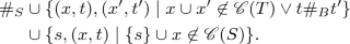
A dependency graph over $\varGamma \vdash B$ is an event structure G along with a labelling map where any two events $s, s' \in G$ labelled $\textsf {Rtn}\,$ are in conflict, and all maximal configurations of G are of the form [r] for $r \in G$ a return event.

The condition on return events ensures that in any configuration of G there is at most one return event. Events of G are called static events.

We use dependency graphs as a causal representation of programs, reflecting the dependency between different parts of the program. In what follows we enrich this representation with runtime information in order to keep track of the dataflow of the program (in Sect. 3.3), and the associated distributions (in Sect. 3.4).

3.3 Runtime Values and Dataflow Graphs

We have seen how data dependency can be captured by representing a program P as a dependency graph $G_P$. But observe that this graph does not give any runtime information about the data in P; every event $s \in G_P$ only carries a label $\textsf {lbl}(s)$ indicating the class of action it belongs to. (For an event labelled $\textsf {Rd}\, a\,$, G does not specify the value at a; whereas at runtime this will be filled by an element of $\llbracket A \rrbracket$ where A is the type of a.)

To each label, we can associate a measurable space of possible runtime values:

Then, in a particular execution, an event $s \in G_P$ has a value in , and can be instead labelled by the following expanded set:

$$\mathscr {L}^{\texttt {run}}_{\varGamma \vdash B} {{:}{:}}= \textsf {Rd}\, a\, v \mid \textsf {Rtn}\, v \mid \textsf {Sam}\, r \mid \textsf {Sco}\, r$$

where r ranges over real numbers; in $\textsf {Rd}\, a\, v$, $a: A \in \varGamma$ and $v \in \llbracket {A}\rrbracket$; and in $\textsf {Rtn}\, v$, v ranges over elements of $\llbracket {B}\rrbracket$. Notice that there is an obvious forgetful map $\alpha : \mathscr {L}^{\texttt {run}}_{\varGamma \vdash A} \rightarrow \mathscr {L}^{\texttt {static}}_{\varGamma \vdash A}$, discarding the runtime value. This runtime value can be extracted from a label in $\mathscr {L}^{\texttt {run}}_{ \varGamma \vdash B}$ as follows:

$$\mathbf q(\textsf {Rd}\, b\, v) = v\qquad \mathbf q(\textsf {Rtn}\, v) = v \qquad \mathbf q(\textsf {Sam}\, r) = r \qquad \mathbf q(\textsf {Sco}\, r) = r.$$

In particular, we have .

Such runtime events organise themselves in an event structure $E_P$, labelled over $\mathscr {L}^{\texttt {run}}_{\varGamma \vdash B}$, the runtime graph of P. Runtime graphs are in general uncountable, and so difficult to represent pictorially. It can be done in some simple, finite cases: the graph for is depicted on the right. Recall that in dependency graphs conflict was used to represent conditional branches; here instead conflict is used to keep disjoint the possible outcomes of the same static event. (Necessarily, this static event must be a sample or a read, since other actions (return, score) are deterministic.)

Intuitively one can project runtime events to static events by erasing the runtime information; this suggests the existence of a function . This function will turn out to satisfy the axioms of a rigid map of event structures:

Definition 3

Given event structures $(E, \le _E, \#_E)$ and $(G, \le _G, \#_G)$ a function $\pi : E \rightarrow G$ is a rigid map if

• it preserves configurations: for every $x \in \mathscr {C}(E)$, $\pi x \in \mathscr {C}(G)$

• it is locally injective: for every $x \in \mathscr {C}(E)$ and $e, e' \in x$, if $\pi (e) = \pi (e')$ then $e = e'$.

• it preserves dependency: if $e \le _E e'$ then $\pi (e) \le _G \pi (e').$

In general $\pi$ is not injective, since many runtime events may correspond to the same static event – in that case however the axioms will require them to be in conflict. The last condition in the definition ensures that all causal dependencies come from G.

Given we define the possible runtime values for x as the set of functions mapping $s \in x$ to a runtime value in ; in other words . A configuration $x'$ of $E_P$ can be viewed as a trace over $\pi _P \, x'$; hence is the set of traces of P over x. We can now define dataflow graphs:

Definition 4

A dataflow graph on $\varGamma \vdash B$ is a triple with $G_S$ a dependency graph and $E_S$ a runtime graph, such that:

• $\pi _S$ is a rigid map and

• for each $x \in \mathscr {C}(G_S)$, the following function is injective

  

• if $e, e' \in E_S$ with then $\pi e = \pi e'$, and moreover e and $e'$ are either both sample or both read events.

As mentioned above, maximal configurations of $E_P$ correspond to total traces of P, and will be the states of the Markov chain in Sect. 5. By the second axiom, they can be seen as pairs . Because of the third axiom, $E_S$ is always confusion-free.

Measurable Fibres. Rigid maps are convenient in this context because, they allow for reasoning about program traces by organising them as fibres. The key property we rely on is the following:

Lemma 2

If $\pi : E \rightarrow G$ is a rigid map of event structures, then the induced map $\pi : \mathscr {C}(E) \rightarrow \mathscr {C}(G)$ is a discrete fibration: that is, for every $y \in \mathscr {C}(E)$, if $x \subseteq \pi y$ for some $x \in \mathscr {C}(G)$, then there is a unique $y' \in \mathscr {C}(E)$ such that $y' \subseteq y$ and $\pi y' = x$.

This enables an essential feature of our approach: given a configuration x of the dataflow graph G, the fibre $\pi ^{-1}\{x\}$ over it contains all the (possibly partial) program traces over x, i.e. those whose path through the program corresponds to that of x. Additionally the lemma implies that every pair of configurations $x, x' \in \mathscr {C}(G)$ such that $x \subseteq x'$ induces a restriction map $r_{x, x'} : \pi ^{-1}\{x'\} \rightarrow \pi ^{-1}\{x\}$, whose action on a program trace over $x'$ is to return its prefix over x.

Although there is no measure-theoretic structure in the definition of dataflow graphs, we can recover it: for every $x \in \mathscr {C}(G_S)$, the fibre $\pi _S^{-1}\{x\}$ can be equipped with the $\sigma$-algebra induced from via $q_x$; it is generated by sets $q_x^{-1} {U}$ for .

It is easy to check that this makes the restriction map $r_{x, x'} : \pi _S^{-1}\{x'\} \rightarrow \pi _S^{-1}\{x\}$ measurable for each pair $x, x'$ of configurations with $x \subseteq x'$. (Note that this makes $\mathbf S$ a measurable event structure in the sense of [16].) Moreover, the map , mapping $x' \in \pi _S^{-1}\{x\}$ to $\mathbf q(\textsf {lbl}(s'))$ for $s'$ the unique antecedent by $\pi _S$ of s in $x'$, is also measurable.

We will also make use of the following result:

Lemma 3

Consider a dataflow $\mathbf S$ and $x, y, z \in \mathscr {C}(G_S)$ with $x \subseteq y$, $x \subseteq z$, and $y \cup z \in \mathscr {C}(G_S)$. If $y \cap z = x$, then the space $\pi _S^{-1}\{y \cup z\}$ is isomorphic to the set

$$\{ (u_y, u_z) \in \pi _S^{-1}\{y\} \times \pi _S^{-1}\{z\} \mid r_{x, y}(u_y) = r_{x, z}(u_z) \},$$

with $\sigma$-algebra generated by sets of the form $\{ (u_y, u_z) \in X_y \times X_z \mid X_y \in \varSigma _{ \pi _S^{-1}\{y\}}, X_z \in \varSigma _{ \pi _S^{-1}\{z\}} \text { and } r_{x, y}(u_y) = r_{x, z}(u_z)$ $\}$.

(For the reader with knowledge of category theory, this says exactly that the diagram

is a pullback in the category of measurable spaces.)

3.4 Quantitative Dataflow Graphs

We can finally introduce the last bit of information we need about programs in order to perform inference: the probabilistic information. So far, in a dataflow graph, we know when the program is sampling, but not from which distribution. This is resolved by adding for each sample event s in the dependency graph a kernel $k_s : \pi ^{-1}\{[s)\} \rightsquigarrow \pi ^{-1}\{[s]\}$. Given a trace x over [s), $k_s$ specifies a probability distribution according to which x will be extended to a trace over [s]. This distribution must of course have support contained in the set $r_{[s), [s]}^{-1}\{x\}$ of traces over [s] of which x is a prefix; this is the meaning of the technical condition in the definition below.

Definition 5

A quantitative dataflow graph is a tuple where for each sample event $s \in G_S$, $k^S_s$ is a kernel $\pi ^{-1}\{[s)\} \rightsquigarrow \pi ^{-1}\{[s]\}$ satisfying for all $x \in \pi ^{-1}\{[s)\},$

$$k_s^S (x, \pi ^{-1}\{[s]\} \setminus r^{-1}_{[s), [s]}\{x\}) = 0.$$

This axiom stipulates that any extension $x' \in \pi _S^{-1}\{[s]\}$ of $x \in \pi _S^{-1}\{[s)\}$ drawn by $k_s$ must contain x; in effect $k_s$ only samples the runtime value for s.

From Graphs to Kernels. We show how to collapse a quantitative dataflow graph $\mathbf S$ on $\varGamma \vdash B$ to a kernel $\llbracket \varGamma \rrbracket \rightsquigarrow \llbracket B \rrbracket$. First, we extend the kernel family on sampling events $(k^S_s : \pi ^{-1}\{[s)\} \rightsquigarrow \pi ^{-1}\{[s]\})$ to a family $(k^{S[ \gamma ]}_s : \pi ^{-1}\{[s)\} \rightsquigarrow \pi ^{-1}\{[s]\})$ defined on all events $s \in S$, parametrised by the value of the environment . To define $k^{S[ \gamma ]}_s(x, \cdot )$ it is enough to specify its value on the generating set for $\varSigma _{ \pi ^{-1}\{[s]\}}$. As we have seen this contains elements of the form $q_{[s]}^{-1} (U)$ with . We distinguish the following cases corresponding to the nature ofs:

• If s is a sample event, $k_s^{S[ \gamma ]} = k_s^S$

• If s is a read on a : A, any $x \in \pi ^{-1}[s)$ has runtime information $q_{[s)}(x)$ in which can be extended to by mapping s to $\gamma (a)$:

  $$k^{S[ \gamma ]}_s(x, q_{[s]}^{-1}U) = \delta _{q_{[s)}(x)[s:= \gamma (a)]}(U)$$

• If s is a return or a score event: any $x \in \pi ^{-1}\{[s)\}$ has at most one extension to $o(x) \in \pi ^{-1}\{[s]\}$ (because return and score events cannot be involved in a minimal conflict): $k^{S[ \gamma ]}_s (x, q_{[s]}^{-1}(U)) = \delta _{q_{[s]}(o(x))}(U).$ If o(x) does not exist, we let $k_s^{S[ \gamma ]}(x, X) = 0$.

We can now define a kernel $k^{S[ \gamma ]}_{x, s} : \pi ^{-1}\{x\} \rightsquigarrow \pi ^{-1} \{x'\}$ for every atomic extension in $G_S$, ie. when $x' \setminus x = \{s\}$, as follows:

$$k^{S[ \gamma ]}_{x, s}(y, U) = k_s(r_{[s), x}(y), \{ w \in \pi _S^{-1}\{[s]\} \mid (y, w) \in U\}).$$

The second argument to $k_s$ above is always measurable, by a standard measure-theoretic argument based on Lemma 3, as $x \cap [s] = [s)$.

From this definition we derive:

Lemma 4

If and are concurrent extensions of x (i.e. $s_1$ and $s_2$ are not in conflict), then $k^{S[ \gamma ]} _{x_1, s_2} \circ k^{S[ \gamma ]} _{x, s_1} = k^{S[ \gamma ]} _{x_2, s_1} \circ k^{S[ \gamma ]} _{x, s_2}$.

Given a configuration and a covering chain , we can finally define a measure on $\pi ^{-1}\{x\}$:

$$ \mu ^{S[ \gamma ]}_{x} = k^{S[ \gamma ]}_{x_{n-1}, s_n} \circ \ldots \circ k^{S[ \gamma ]}_{\emptyset , s_1}(*, \cdot ),$$

where $*$ is the only trace over $\emptyset$. The particular covering chain used does not matter by the previous lemma. Using this, we can define the kernel of a quantitative dataflow graph $\mathbf S$ as follows:

$$\textsf {kernel}(\mathbf S)( \gamma , X) = \sum _{r \in G_S, \textsf {lbl}(r) = \textsf {Rtn}\, } \mu ^{S[ \gamma ]}_{[r]}(q_{[r], r}^{-1}(X)),$$

where the measurable map looks up the runtime value of r in an element of the fibre over [r] (defined in Sect. 3.3).

Lemma 5

$\textsf {kernel}(\mathbf S)$ is an s-finite kernel $\llbracket \varGamma \rrbracket \rightsquigarrow \llbracket B \rrbracket$.

4 Programs as Labelled Event Structures

We now detail our interpretation of programs as quantitative dataflow graphs. Our interpretation is given by induction, similarly to the measure-theoretic interpretation given in Sect. 2.3, in which composition of kernels plays a central role. In Sect. 4.1, we discuss how to compose quantitative dataflow graphs, and in Sect. 4.2, we define our interpretation.

4.1 Composition of Probablistic Event Structures

Consider two quantitative dataflow graphs, S on $\varGamma \vdash A$, and T on $\varGamma , a:A \vdash B$ where a does not occur in $\varGamma$. In what follows we show how they can be composed to form a quantitative dataflow graph $T \odot ^{a}_{} S$ on $\varGamma \vdash B$.

Unlike in the kernel model of Sect. 2.3, we will need two notions of composition. The first one is akin to the usual sequential composition: actions in T must wait on S to return before they can proceed. The second is closer to parallel composition: actions on T which do not depend on a read of the variable a can be executed in parallel with S. The latter composition is used to interpret the let construct. In , we want all the probabilistic actions or reads on other variables which do not depend on the value of a to be in parallel with M. However, in a program such as we do not want any actions of $N_i$ to start before the selected branch is known, i.e. before the return value of M is known.

By way of illustration, consider the following simple example, in which we only consider runtime graphs, ignoring the rest of the structure for now. Suppose S and T are given by

The graph S can be seen to correspond to the program and T to the pairing for any d. Here S is a runtime graph on $b: \mathbb B\vdash \mathbb B$ and T on $a: \mathbb B, b: \mathbb B\vdash \mathbb B$.

Both notions of compositions are displayed in the diagram below. The sequential composition (left) corresponds to

and the parallel composition to :

Composition of Runtime and Dependency Graphs. Let us now define both composition operators at the level of the event structures. Through the bijection $\mathscr {L}^{\texttt {static}}_{ \varGamma \vdash B} \simeq \mathscr {L}^{\texttt {run}}_{ \varGamma ' \vdash 1}$ where $\varGamma '(a) = 1$ for all $a \in \text {dom}( \varGamma )$, we will see dependency graphs and runtime graphs as the same kind of objects, event structures labelled over $\mathscr {L}^{\texttt {run}}_{ \varGamma \vdash A}$.

The two compositions $S \odot ^{a}_{\text {par}} T$ and $S \odot ^{a}_{\text {seq}} T$ are two instances of the same construction, parametrised by a set of labels $D \subseteq \mathscr {L}^{\texttt {run}}_{\varGamma , a: A \vdash B}$. Informally, D specifies which events of T are to depend on the return value of S in the resulting composition graph. It is natural to assume in particular that D contains all reads on a, and all return events.

Sequential and parallel composition are instances of this construction where D is set to one of the following:

$$ \begin{aligned} D^{ \varGamma , a: A \vdash B}_{\text {seq}} = \mathscr {L}^{\texttt {run}}_{ \varGamma , a: A \vdash B} \qquad \qquad D^{ \varGamma , a: A \vdash B}_{\text {par}} = \{ \textsf {Rd}\, a\, v, \textsf {Rtn}\, v \in \mathscr {L}^{\texttt {run}}_{ \varGamma , a: A \vdash B} \}. \end{aligned}$$

We proceed to describe the construction for an abstract D. Let T be an event structure labelled by $\mathscr {L}^{\texttt {run}}_{ \varGamma , a: A \vdash B}$ and S labelled by $\mathscr {L}^{\texttt {run}}_{ \varGamma \vdash A}$. A configuration is a justification of when

• 1. if $\textsf {lbl}(y)$ intersects D, then x contains a return event

• 2. for all $t \in y$ with label $\textsf {Rd}\, a\, v$, there exists an event $s \in x$ labelled $\textsf {Rtn}\, v$.

In particular if $\textsf {lbl}(y)$ does not intersect D, then any configuration of S is a justification of y. A minimal justification of y is a justification that admits no proper subset which is also a justification of y. We now define the event structure $S \cdot _D T$ as follows:

• Events: ;

• Causality: $\le _S\ \cup \ \{ (x, t), (x', t') \mid x \subseteq x' \wedge t \le t' \}\ \cup \ \{ s, (x, t) \mid s \in x \}$;

• Conflict: the symmetric closure of

  

Lemma 6

$S \cdot _D T$ is an event structure, and the following is an order-isomorphism:

This event structure is not quite what we want, since it still contains return events from S and reads on a from T. To remove them, we use the following general construction. Given a $\varSigma$-labelled event structure E and $V \subseteq E$ a set of visible events, its projection $E \downarrow V$ has events V and causality, conflict and labelling inherited from E. Thus the composition of S and T is:

$$S \odot ^{a}_{D} T := S \cdot _D T \downarrow (\{ s \in S \mid ~s \text { not a return}\} \cup \{ (x, t) \mid ~t \text { not a read on } a\}).$$

As a result $S \odot ^{a}_{D} T$ is labelled over $\mathscr {L}^{\texttt {run}}_{ \varGamma \vdash B}$ as needed.

Dataflow Information. We now explain how this construction lifts to dataflow graphs. Consider dataflow graphs on $\varGamma \vdash A$ and on $\varGamma , a: A \vdash B$. Given $D \subseteq \mathscr {L}^{\texttt {static}}_{ \varGamma , a: A \vdash B}$ we define

$$ \begin{aligned} E_{S \cdot _D T}&= E_S \cdot _{ \alpha ^{-1}D} E_T&\qquad G_{S \cdot _D T}&= G_S \cdot _D G_T \\ E_{S \odot ^{a}_{D} T}&= E_{S} \odot ^{a}_{ \alpha ^{-1}D} E_T&\qquad G_{S \odot ^{a}_{D} T}&= G_S \odot ^{a}_{D} G_T \\ \end{aligned} $$

Lemma 7

The maps $\pi _S$ and $\pi _T$ extend to rigid maps

Moreover, if , $\langle \pi _S\, x, \pi _T\, y \rangle$ is a well-defined configuration of $G_{S \cdot _D T}$. As a result, for , we have a injection making the following diagram commute:

In particular, $\varphi _{x, y}$ is measurable and induces the $\sigma$-algebra on $\pi ^{-1}\{\langle x, y \rangle \}$. We write $\varphi _x$ for the map $\varphi _{x, \emptyset }$, an isomorphism.

Adding Probability. At this point we have defined all the components of dataflow graphs $S \odot ^{a}_{D} T$ and $S \cdot _D T$. We proceed to make them quantitative.

Observe first that each sampling event of $G_{S \cdot _D T}$ (or equivalently of $G_{S \odot ^{a}_{D} T}$ – sampling events are never hidden) corresponds either to a sampling event of $G_S$, or to an event (x, t) where t is a sampling event of $G_T$. We consider both cases to define a family of kernels $(k_s^{S \cdot _D T})$ between the fibres of $S\cdot _D T$. This will in turn induce a family $(k_s^{S \odot ^{a}_{D} T})$ on $S\odot ^{a}_{D} T$.

• If s is a sample event of $G_S$, we use the isomorphisms $\varphi _{[s)}$ and $\varphi _{[s]}$ of Lemma 7 to define:

  $$k_s^{S \odot ^{a}_{D} T} (v, X) = k_s^S ( \varphi ^{-1}_{[s)}\, v, \varphi ^{-1}_{[s]} X).$$

• If s corresponds to (x, t) for t a sample event of $G_T$, then for every $X_x \in \varSigma _{ \pi _S^{-1}\{x\}}$ and $X_t \in \varSigma _{ \pi ^{-1}_T\{[t)\}}$ we define

  $$k_{(x, t)}^{S \odot ^{a}_{D} T} ( \langle x', y' \rangle , \varphi ^{-1}_{x, [t]}( X_x \times X_t )) = \delta _{x'}(X_x) \times k_t^T(y', X_t).$$

  By Lemma 7, the sets $\varphi ^{-1}_{x, [t]}( X_x \times X_t )$ form a basis for $\varSigma _{\pi ^{-1}\{\langle x, [t)\}}$, so that this definition determines the entire kernel.

So we have defined a kernel $k_s^{S\cdot _D T}$ for each sample event s of $G_{S\cdot _D T}$. We move to the composition $(S \odot ^{a}_{D} T).$ Recall that the causal history of a configuration is the set [z], a configuration of $G_{S \cdot _D T}$. We see that hiding does not affect the fibre structure:

Lemma 8

For any , there is a measurable isomorphism $\psi _z: \pi _{S \odot ^{a}_{D} T}^{-1}\{z\} \cong \pi _{S \cdot _D T}^{-1}\{[z]\}$.

Using this result and the fact that $G_{S \odot ^{a}_{D} T} \subseteq G_{S \cdot _D T}$, we may define for each s:

$$k^{S \odot ^{a}_{D} T}_s(v, X) = k^{S \cdot _D T}_s ( \psi _{[s)}(v), \psi _{[s]} X).$$

We conclude:

Lemma 9

${S}\odot ^{a}_{D} T := (G_{S \odot ^{a}_{D} T}, E_{S\odot ^{a}_{D} T}, \pi _{S\odot ^{a}_{D} T}, (k_s^{S\odot ^{a}_{D} T}))$ is a quantitative dataflow graph on $\varGamma \vdash B$.

Multicomposition. By chaining this composition, we can compose on several variables at once. Given quantitative dataflow graphs $S_i$ on $\varGamma \vdash A_i$ and T on $\varGamma , a_1:A_1, \ldots , a_n: A_n \vdash A$ we define

$$ \begin{aligned} (S_i) \odot ^{(a_i)}_{\text {par}} T := S_1 \odot ^{a_1}_{\text {par}} ( \ldots \odot ^{a_n}_{\text {par}} T)\\ (S_i) \odot ^{(a_i)}_{\text {seq}} T := S_1 \odot ^{a_1}_{\text {seq}} ( \ldots \odot ^{a_n}_{\text {seq}} T)\\ \end{aligned}$$

4.2 Interpretation of Programs

We now describe how to interpret programs of our language using quantitative dataflow graphs. To do so we follow the same pattern as for the measure-theoretical interpretation given in Sect. 2.3.

Interpretation of Functions. Given a measurable function , we define the quantitative dataflow graph

We then define $\llbracket {f\, M}\rrbracket _{\mathcal G}$ as $\llbracket {M}\rrbracket _{\mathcal G} \odot ^{a}_{\text {par}} {S^a_f}$ where a is chosen so as not to occur free in M.

Probablistic Actions. In order to interpret scoring and sampling primitives, we need the following two quantitative dataflow graphs:

and we define $k_{\textsf {Sam}}$ by integrating the density function d; here we identify and $\pi ^{-1}\{\{\textsf {Rd}\, a\, , \textsf {Sam}\}\}$:

$$k_{\textsf {Sam}} (\{\textsf {Rd}\, a\, \mathbf r\}, U) = \int _{\begin{array}{c} q \in U, q(\textsf {Rd}\, a\, \!) = \mathbf {r} \end{array}} d(\mathbf r, q(\textsf {Sam})) \mathrm {d}\lambda .$$

We can now interpret scoring and sampling constructs:

Interpretation of Tuples and Variables. Given a family $(a_i)_{i \in I}$, we define the dataflow graph $\texttt {tuple}_{(a_i:A_i)}$ on $a_1: A_1, \ldots , a_n: A_n \vdash A_1 \times \ldots \times A_n$ as follows. Its set of events is the disjoint union

where the conflict is induced by for $v \ne v'$; and causality contains all the pairs where $v_i = v$. Then we form a quantitative dataflow graph $\texttt {Tuple}_{(a_i: A_i)}$, whose dependency graph is $\mathtt {tuple}_{(a_i: 1)}$ (up to the bijection $\mathscr {L}^{\texttt {run}}_{ \varGamma \vdash A} \simeq \mathscr {L}^{\texttt {static}}_{ \varGamma ' \vdash 1}$ where $\varGamma '(a) = 1$ for $a \in \text {dom}( \varGamma )$); and the runtime graph is $\mathtt {tuple}_{(a_i: A_i)}$, along with the obvious rigid map between them.

We then define the semantics of $(M_1, \ldots , M_n)$:

where the $a_i$ are chosen free in all of the $M_j$. This construction is also useful to interpret variables:

Interpretation of Pattern Matching. Consider now a term of the form . By induction, we have that is a quantitative dataflow graph on $\varGamma , a: A_i \vdash B$. Let us write for the quantitative dataflow graph on $\varGamma , a: (\sum _{i \in I} A_i) \vdash B$ obtained by relabelling events of the form $\textsf {Rd}\, a\, v$ to $\textsf {Rd}\, a\, (i, v)$, and sequentially precomposing with $\texttt {Tuple}_{a: \sum _{i \in I} A_i}$. This ensures that minimal events in are reads on a. We then build the quantitative dataflow graph on $\varGamma , a: \sum _{i \in I} A_i \vdash B$. This can be composed with :

It is crucial here that one uses sequential composition: none of the branches must be evaluated until the outcome of M is known.

Adequacy of Composition. We now prove that our interpretation is adequate with respect to the measure-theoretic semantics described in Sect. 2.3. Given any subset $D \subseteq {\mathscr {L}^{\texttt {static}}_{ \varGamma , a: A \vdash B}}$ containing returns and reads on a, we show that the composition ${S}\odot ^{a}_{D} T$ does implement the composition of kernels:

Theorem 1

For S a quantitative dataflow graph on $\varGamma \vdash A$ and T on $\varGamma , a: A \vdash B$, we have

From this result, we can deduce that the semantics in terms of quantitative dataflow graphs is adequate with respect to the measure-theoretic semantics:

Theorem 2

For every term $\varGamma \vdash M: A$, $\textsf {kernel}( \llbracket {M}\rrbracket _{\mathcal G}) = \llbracket {M}\rrbracket$.

5 An Inference Algorithm

In this section, we exploit the intensional semantics defined above and define a Metropolis-Hastings inference algorithm. We start, in Sect. 5.1, by giving a concrete presentation of those quantitative dataflow graphs arising as the interpretation of probabilistic programs; we argue this makes them well-suited for manipulation by an algorithm. Then, in Sect. 5.2, we give a more formal introduction to the Metropolis-Hastings sampling methods than that given in Sect. 3. Finally, in Sect. 5.3, we build the proposal kernel on which our implementation relies, and conclude.

5.1 A Concrete Presentation of Probabilistic Dataflow Graphs

Quantitative dataflow graphs as presented in the previous sections are not easy to handle inside of an algorithm: among other things, the runtime graph has an uncountable set of events. In this section we show that some dataflow graphs, in particular those needed for modelling programs, admit a finite representation.

Recovering Fibres. Consider a dataflow graph $\mathbf S = (E_S, G_S, \pi _S)$ on $\varGamma \vdash B$. It follows from Lemma 3 that the fibre structure of $\mathbf S$ is completely determined by the spaces $\pi _S^{-1}\{[s]\}$, for $s \in G_S$, so we focus on trying to give a simplified representation for those spaces.

First, let us notice that if s is a return or score event, given $x \in \pi ^{-1}\{x\}$, the value $q_x(s)$ is determined by $q\vert _{[s)}$. In other words the map is an injection. This is due to the fact that minimal conflict in $E_S$ cannot involve return or score events. As a result, $E_S$ induces a partial function , called the outcome function. It is defined as follows:

$$o^S_s(q) = \left\{ \begin{aligned}&q_{[s]} (x')(s)\qquad&\text {if there exists } x' \in \pi ^{-1}\{x'\}, q_{[s]}(x')\vert _{[s)} = q,\\&\text {undefined}\qquad&\text {otherwise.} \end{aligned}\right. $$

Note that $x'$ must be unique by the remark above since its projection to is determined by q. The function $o^S$ is partial, because it might be the case that the event s occurs conditionally on the runtime value on [s).

In fact this structure is all we need in order to describe a dataflow graph:

Lemma 10

Given $G_S$ a dependency graph on $\varGamma \vdash B$, and partial functions for score and return events of S. There exists a dataflow graph whose outcome functions coincide with the $o_s$. Moreover, there is an order-isomorphism

Adding Probabilities. To add probabilities, we simply equip each sample event s of $G_S$ with a density function .

Definition 6

A concrete quantitative dataflow graph is a tuple where $d_s(x, \cdot )$ is normalised.

Lemma 11

Any concrete quantitative dataflow graph $\mathcal S$ unfolds to a quantitative dataflow graph .

We see now that the quantitative dataflow graphs arising as the interpretation of a program must be the unfolding of a concrete quantitative dataflow graph:

Lemma 12

For any concrete quantitative dataflow graphs $\mathcal S$ on $\varGamma \vdash A$ and $\mathcal T$ on $\varGamma , a: A \vdash B$, is the unfolding of a concrete quantitative dataflow graph. It follows that for any program $\varGamma \vdash M : B$, is the unfolding of a concrete quantitative dataflow graph.

5.2 Metropolis-Hastings

Recall that the Metropolis-Hastings algorithm is used to sample from a density function which may not be normalised. Here $\mathbb A$ is a measurable state space, equipped with a measure $\lambda$. The algorithm works by building a Markov chain whose stationary distribution is D, the probability distribution obtained from d after normalisation:

$$ \forall X \in \varSigma _{\mathbb A}, D(X) = \frac{\int _{x \in X}d(x)}{\int _{x \in \mathbb A} d(x)}.$$

Our presentation and reasoning in the rest of this section are inspired by the work of Borgström et al. [2].

Preliminaries on Markov Chains. A Markov chain on a measurable state space $\mathbb A$ is a probability kernel $k: \mathbb A \rightsquigarrow \mathbb A$, viewed as a transition function: given a state $x \in \mathbb A$, the distribution $k(x, \cdot )$ is the distribution from which a next sample state will be drawn. Usually, each $k(x, \cdot )$ comes with a procedure for sampling: we will treat this as a probabilistic program M(x) whose output is the next state. Given an initial state $x \in \mathbb A$ and a natural number $n \in \mathbb N$, we have a distribution $k^n(x, \cdot )$ on $\mathbb A$ obtained by iterating k n times. We say that the Markov chain k has limit the distribution $\mu$ on $\mathbb A$ when

$$\lim _{n\rightarrow \infty }||k^n(x, \cdot ) - \mu || = 0 \qquad \text {where } || \mu _1 - \mu _2|| = \sup _{A \in \varSigma _{\mathbb A}} \mu _1(A) - \mu _2(A).$$

For the purposes of this paper, we call a Markov chain computable when there exists a type A such that $\llbracket A \rrbracket = \mathbb A$ (up to iso) and an expression without scores $x: A \vdash K: A$ such that $\llbracket K \rrbracket = k$. (Recall that programs without conditioning denote probabilistic kernels, and are easily sampled from, since all standard distributions in the language are assumed to come with a built-in sampler.)

We will use terms of our language to describe computable Markov chains language, taking mild liberties with syntax. We assume in particular that programs may call each other as subroutines (this can be done via substitutions), and that manipulating finite structures is computable and thus representable in the language.

The Metropolis-Hastings Algorithm. Recall that we wish to sample from a distribution with un-normalised density ; d is assumed to be computable. The Markov chain defined by the Metropolis-Hastings algorithm has two parameters: a computable Markov chain $x: A \vdash P: A$, the proposal kernel, and a measurable, computable function representing the kernel $\llbracket P \rrbracket$, i.e.

$$ \llbracket P \rrbracket (x, X') = \int _{x' \in X'} p(x, x') \,d\lambda (x').$$

The Markov-chain $\texttt {MH}(P, p, d)$ is defined as

In words, the Markov chain works as follows: given a start state x, it generates a proposal for the next state $x'$ using P. It then computes an acceptance ratio $\alpha$, which is the probability with which the new sample will be accepted: the return state will then either be the original x or $x'$, accordingly.

Assuming P and p satisfy a number of conditions, the algorithm is correct:

Theorem 3

Assume that P and p satisfies the following properties:

• 1. Strong irreducibility: There exists $n \in \mathbb {N}$ such that for all $x \in \mathbb A$ and $X \in \varSigma _{\mathbb A}$ such that $D(X) \ne \emptyset$ and $d(x) > 0$, there exists $n \in \mathbb {N}$ such that .

• 2.

• 3. If $d(x) > 0$ and $p(x, y) > 0$ then $d(y) > 0$.

• 4. If $d(x) > 0$ and $d(y) > 0$, then $p(x, y) > 0$ iff $p(y, x) > 0$.

Then, the limit of $\texttt {MH}(P, p, d)$ for any initial state $x \in \mathbb A$ with $d(x) > 0$ is equal to D, the distribution obtained after normalising d.

5.3 Our Proposal Kernel

Consider a closed program $\vdash M : A$ in which every measurable function is a computable one. Then, its interpretation as a concrete quantitative dataflow graph is computable, and we write $\mathcal S$ for the quantitative dataflow graph whose unfolding is . Moreover, because M is closed, its measure-theoretic semantics gives a measure $\llbracket M \rrbracket$ on $\llbracket A \rrbracket$. Assume that is well-defined: it is a probability distribution on $\llbracket A \rrbracket$. We describe how a Metropolis-Hastings algorithm may be used to sample from it, by reducing this problem to that of sampling from configurations of $E_S$ according to the following density:

$$d_S (x, q) := \left( \prod _{s \in \text {sample}(x)} d_s(q(s))\right) \left( \prod _{s \in \text {score}(x)} q(s)\right) .$$

Lemma 10 induces a natural measure on $\mathscr {C}(E_S)$. We have:

Lemma 13

For all $X \in \varSigma _{\mathscr {C}(E_S)}$, $\displaystyle {\mu ^{\mathcal S} (X) = \int _{y \in X} d_S(y) \mathrm {d}y.}$

Note that $d_S(x, q)$ is easy to compute, but it is not normalised. Computing the normalising factor is in general intractable, but the Metropolis-Hastings algorithm does not require the density to be normalised.

Let us write for the normalised distribution. By adequacy, we have for all $X \in \varSigma _{ \llbracket A \rrbracket }$:

where maps a maximal configuration of $E_S$ to its return value, if any. This says that sampling from amounts to sampling from $\mu ^{\mathcal S}_{\text {norm}}$ and only keeping the return value.

Accordingly, we focus on designing a Metropolis-Hastings algorithm for sampling values in following the (unnormalised) density $d_S$. We start by defining a proposal kernel for this algorithm.

To avoid overburdening the notation, we will no longer distinguish between a type and its denotation. Since $G_S$ is finite, it can be represented by a type, and so can . Moreover, is a subset of $\sum _{x \in \mathscr {C}(G_S)} \mathscr {Q}(x)$ which is also representable as the type of pairs . Operations on $G_S$ and related objects are all computable and measurable so we can directly use them in the syntax. In particular, we will make use of the function which for each configuration returns $(1, \mathfrak s)$ if there exists with $o_s(q\vert _{[s)})$ defined, and $(2, *)$ if (x, q) is maximal.

Informally, for , the algorithm is:

• Pick a sample event $s \in x$, randomly over the set of sample events of x.

• Construct .

• Return a maximal extension $(x', q')$ of $(x_0, q\vert _{x_0})$ by only resampling the sample events of $x'$ which are not in x.

The last step follows the single-site MH principle: sample events in $x \cap x'$ have already been evaluated in x, and are not updated. However, events which are in $x' \setminus x$ belong to conditional branches not explored in x; they must be sampled.

We start by formalising the last step of the algorithm. We give a probabilistic program complete which has three parameters: the original configuration (x, q), the current modification $(x_0, q_0)$ and returns a possible maximal extension:

The program starts by trying to extend $(x_0, q_0)$ by calling $\texttt {ext}$. If $(x_0, q_0)$ is already maximal, we directly return it. Otherwise, we get an event s. To extend the quantitative information, there are three cases:

• if s is not a sample event, ie. since S is closed it must be a return or a score event, we use the function $o_s$.

• if s is a sample event occurring in x, we use the value in q

• if s is a sample event not occurring in x, we sample a value for it.

This program is recursive, but because $G_S$ is finite, there is a static bound on the number of recursive calls; thus this program can be unfolded to a program expressible in our language. We can now define the proposal kernel:

We now need to compute the density for $P_S$ to be able to apply Metropolis-Hastings. Given , we define:

$$p_S((x, q), (x', q')) = \sum _{s \in \text {sample}(x)} \left( \frac{q_s(v'\vert _{[s)})}{|\text {sample}(x)|} \times \prod _{s' \in \mathtt {sample}(x' \setminus x)} q_{s'}(v\vert _{[s')})\right) .$$

Theorem 4

The Markov chain $P_S$ and density p satisfy the hypothesis of Theorem 3, as a result for any the distribution tends to $\mu _{\text {norm}}^P$ as n goes to infinity.

One can thus sample from using the algorithm above, keeping only the return value of the obtained configuration.

Let us re-state the key advantage of our approach: having access to the data dependency information, complete requires fewer steps in general, because at each proposal step only a portion of the graph needs exploring.

6 Conclusion

Related Work. There are numerous approaches to the semantics of programs with random choice. Among those concerned with statistical applications of probabilistic programming are Staton et al. [18, 19], Ehrhard et al. [7], and Dahlqvist et al. [6]. A game semantics model was announced in [15].

The work of Scibior et al. [17] was influential in suggesting a denotational approach for proving correctness of inference, in the framework of quasi-Borel spaces [9]. It is not clear however how one could reason about data dependencies in this framework, because of the absence of explicit causal information.

Hur et al. [11] gives a proof of correctness for Trace MCMC using new forms of operational semantics for probabilistic programs. This method is extended to higher-order programs with soft constraints in Borgström et al. [2]. However, these approaches do not consider incremental recomputation.

To the best of our knowledge, this is the first work addressing formal correctness of incremental recomputation in MCMC. However, methods exist which take advantage of data dependency information to improve the performance of each proposal step in “naive” Trace MCMC. We mention in particular the work on slicing by Hur et al. [10]; other approaches include [5, 24]. In the present work we claim no immediate improvement in performance over these techniques, but only a mathematical framework for reasoning about the structures involved.

It is worth remarking that our event structure representation is reminiscent of graphical model representation made explicit in some languages. Indeed, for a first-order language such as the one of this paper, Bayesian networks can directly be used as a semantics, see [20]. We claim that the alternative view offered by event structures will allow for an easier extension to higher-order programs, using ideas from game semantics.

Perspectives. This is the start of an investigation into intensional semantics for probabilistic programs. Note that the framework of event structures is very flexible and the semantics presented here is by no means the only possible one. Additionally, though the present work only treats the case of a first-order language, we believe that building on recent advances in probabilistic concurrent game semantics [3, 16] (from which the present work draws much inspiration), we can extend the techniques of this paper to arbitrary higher-order probabilistic programs with recursion.

References

Billingsley, P.: Probability and Measure. John Wiley & Sons, New York (2008)
Borgström, J., Lago, U.D., Gordon, A.D., Szymczak, M.: A lambda-calculus foundation for universal probabilistic programming. In: ACM SIGPLAN Notices, vol. 51, pp. 33–46. ACM (2016)
Castellan, S., Clairambault, P., Paquet, H., Winskel, G.: The concurrent game semantics of probabilistic PCF. In: 2018 33rd Annual ACM/IEEE Symposium on Logic in Computer Science (LICS). ACM/IEEE (2018)
Castellan, S., Paquet, H.: Probabilistic programming inference via intensional semantics. Technical report (2019). http://iso.mor.phis.me/publis/esop19.pdf
Chen, Y., Mansinghka, V., Ghahramani, Z.: Sublinear approximate inference for probabilistic programs. stat, 1050:6 (2014)
Dahlqvist, F., Danos, V., Garnier, I., Silva, A.: Borel kernels and their approximation, categorically. arXiv preprint arXiv:1803.02651 (2018)
Ehrhard, T., Pagani, M., Tasson, C.: Measurable cones and stable, measurable functions: a model for probabilistic higher-order programming, vol. 2, pp. 59:1–59:28 (2018)
Gordon, A.D., Henzinger, T.A., Nori, A.V., Rajamani, S.K.: Probabilistic programming. In: Proceedings of the on Future of Software Engineering, pp. 167–181. ACM (2014)
Heunen, C., Kammar, O., Staton, S., Yang, H.: A convenient category for higher-order probability theory. In: LICS 2017, Reykjavik, pp. 1–12 (2017)
Hur, C.-K., Nori, A.V., Rajamani, S.K., Samuel, S. Slicing probabilistic programs. In: ACM SIGPLAN Notices, vol. 49, pp. 133–144. ACM (2014)
Hur, C.-K., Nori, A.V., Rajamani, S.K., Samuel, S.: A provably correct sampler for probabilistic programs. In: LIPIcs-Leibniz International Proceedings in Informatics, vol. 45. Schloss Dagstuhl-Leibniz-Zentrum fuer Informatik (2015)
Kiselyov, O.: Probabilistic programming language and its incremental evaluation. In: Igarashi, A. (ed.) APLAS 2016. LNCS, vol. 10017, pp. 357–376. Springer, Cham (2016). https://doi.org/10.1007/978-3-319-47958-3_19
Kiselyov, O.: Problems of the lightweight implementation of probabilistic programming. In: Proceedings of Workshop on Probabilistic Programming Semantics (2016)
Kozen, D.: Semantics of probabilistic programs. J. Comput. Syst. Sci. 22(3), 328–350 (1981)
Ong, L., Vákár, M.: S-finite kernels and game semantics for probabilistic programming. In: POPL 2018 Workshop on Probabilistic Programming Semantics (PPS) (2018)
Paquet, H., Winskel, G.: Continuous probability distributions in concurrent games. Electr. Notes Theor. Comput. Sci. 341, 321–344 (2018)
Ścibior, A., et al.: Denotational validation of higher-order Bayesian inference. In: Proceedings of the ACM on Programming Languages, vol. 2(POPL), p. 60 (2017)
Staton, S.: Commutative semantics for probabilistic programming. In: Yang, H. (ed.) ESOP 2017. LNCS, vol. 10201, pp. 855–879. Springer, Heidelberg (2017). https://doi.org/10.1007/978-3-662-54434-1_32
Staton, S., Yang, H., Wood, F.D., Heunen, C., Kammar, O.: Semantics for probabilistic programming: higher-order functions, continuous distributions, and soft constraints. In: Proceedings of LICS 2016, New York, NY, USA, July 5–8, 2016, pp. 525–534 (2016)
van de Meent, J.-W., Paige, B., Yang, H., Wood, F.: An introduction to probabilistic programming. arXiv preprint arXiv:1809.10756 (2018)
Wingate, D., Stuhlmüller, A., Goodman, N.: Lightweight implementations of probabilistic programming languages via transformational compilation. In: Proceedings of the Fourteenth International Conference on Artificial Intelligence and Statistics, pp. 770–778 (2011)
Winskel, G.: Event structures. In: Brauer, W., Reisig, W., Rozenberg, G. (eds.) ACPN 1986. LNCS, vol. 255, pp. 325–392. Springer, Heidelberg (1987). https://doi.org/10.1007/3-540-17906-2_31
Winskel, G.: Distributed probabilistic and quantum strategies. Electr. Notes Theor. Comput. Sci. 298, 403–425 (2013)
Wu, Y., Li, L., Russell, S., Bodik, R.: Swift: compiled inference for probabilistic programming languages. arXiv preprint arXiv:1606.09242 (2016)
Yang, L., Hanrahan, P., Goodman, N.: Generating efficient MCMC kernels from probabilistic programs. In: Artificial Intelligence and Statistics, pp. 1068–1076 (2014)
Acknowledgements
We thank the anonymous referees for helpful comments and suggestions. We also thank Ohad Kammar for suggesting the idea of using causal structures for reasoning about data dependency in this context. This work has been partially sponsored by: EPSRC EP/K034413/1, EP/K011715/1, EP/L00058X/1, EP/N027833/1, EP/N028201/1, and an EPSRC PhD studentship.
Author information
Authors and Affiliations
Corresponding author
Editor information
Editors and Affiliations
Rights and permissions
Open Access This chapter is licensed under the terms of the Creative Commons Attribution 4.0 International License (http://creativecommons.org/licenses/by/4.0/), which permits use, sharing, adaptation, distribution and reproduction in any medium or format, as long as you give appropriate credit to the original author(s) and the source, provide a link to the Creative Commons license and indicate if changes were made.
The images or other third party material in this chapter are included in the chapter's Creative Commons license, unless indicated otherwise in a credit line to the material. If material is not included in the chapter's Creative Commons license and your intended use is not permitted by statutory regulation or exceeds the permitted use, you will need to obtain permission directly from the copyright holder.
Copyright information
© 2019 The Author(s)
About this paper
Cite this paper
Castellan, S., Paquet, H. (2019). Probabilistic Programming Inference via Intensional Semantics. In: Caires, L. (eds) Programming Languages and Systems. ESOP 2019. Lecture Notes in Computer Science(), vol 11423. Springer, Cham. https://doi.org/10.1007/978-3-030-17184-1_12
Download citation
DOI: https://doi.org/10.1007/978-3-030-17184-1_12
Published:
Publisher Name: Springer, Cham
Print ISBN: 978-3-030-17183-4
Online ISBN: 978-3-030-17184-1
eBook Packages: Computer ScienceComputer Science (R0)