Trust and Distrust: On Sense and Nonsense in Big Data

Abstract

Big data is an appealing source and often perceived to bear all sorts of hidden information. Filtering out the gemstones of information besides the rubbish that is equally easy to “deduce” is, however, a nontrivial issue. This position paper will open with the motivating problem of risk estimation for an enterprise, using big data. Our illustrative context here is the synERGY project (“security for cyber-physical value networks Exploiting smaRt Grid sYstems”), which serves as a case study to show the (unexplored) potential, application and difficulties of using big data in practice. The paper first goes into a list of a few general do’s and don’ts about data analytics, and then digs deeper into (semi-) automated risk evaluation via a statistical trust model. Ideally, the trust and hence risk assessment should be interpretable, justified, up-to-date and comprehensible in order to provide a maximum level of information with minimal additional manual effort. The ultimate goal of projects like synERGY is to establish trust in a system, based on observed behavior and its resilience to anomalies. This calls for a distinction of “normal” (in the sense of behavior under expected working conditions) from “abnormal” behavior, and trust can intuitively be understood as the (statistical) expectation of “normal” behavior.

1 Introduction

Trust is a generally familiar, but not a clearly defined term in many contexts. In a simple yet intuitive understanding, trust is the expectation of “correct” behavior (of a system, a person, …). As such, it has some relation to security, since the latter is, in a way, also the assurance that certain requirements are met. Our concern in the following will be security systems. Like in social life, security systems gain trust through their reliable behavior, and lose it in the light of threats or incidents related to the system. To “measure” trust, it is thus necessary to recognize relevant incidents and threats and to find a way of evaluating the impact on the trust in the system. A decent trust model should use the information in a transparent form, so as to support accountability (i.e., the clear identification of reasons for anomalies) and fairness (i.e., trust should not overproportionally depend on single types or sources of information). Transparency is thus hereafter understood as the trust model’s artefacts to be explainable, justifiable and interpretability beyond being only the result of complex computations. Methods lacking this kind of transparency are hereafter called “black-box”. The two kinds may not differ in their power, but only in the degree to which the results can be explained. For security, it may be enough that the system works as expected; however, when it comes to the aftermath of an incident, it may additionally become necessary to understand the reason why the security did not work as expected (which calls for explainability).

Our position paper opens with an example of a security system related to anomaly detection in energy grids. This then shall provide the context for the further discussion of a simple statistical model to quantify trust and to incorporate continuously incoming information about a system into the system’s trust indicator. The aim is to calculate a (always current) confidence index from the history of observed system behavior. The evolution of this trust variable over time is then useful to warn about future risk situations arising from possible series of events that would destroy trust. Worst-case risk, equivalently trust, scenarios then correspond to the shortest sequence of events that makes the trust index drop below a certain threshold (of acceptable risk). One lesson taught by the model is that “fairness” in the sense of how information affects the trust is not necessarily naturally consistent with the human understanding of trust. The statistical trust model is indifferent between positive or negative experience; the trust would change by relatively equal magnitudes into either direction. Between humans, however, trust can be much harder to gain than to lose.

The second part of the paper focuses on the detection of incidents within the history. For this purpose, statistical approaches exist which can uncover an artificial manipulation of data (under suitable conditions). The consideration here lies on the possibility of an automated recognition of manipulations purely on the basis of numerical data and in particular without recourse to (human) domain expertise.

More accurate models of trust as a measure of resilience against or likelihood of abnormal behavior can be established if domain knowledge is available. The statistical toolbox therefor covers a wide spectrum of methods, a categorization of which we will look into in the third part of this tutorial devoted to our case study. Our focus will therein be on reporting practical issues and challenges to overcome when striving for statistical anomaly detection up to predictive analytics.

2 Practical Anomaly Detection by Example – the synERGY Project

The synERGY project [1] aims at constructing an anomaly detection system for energy distribution systems operators (DSOs), which usually maintain highly distributed systems unifying many heterogeneous information technology (IT) and operational technology (OT) components and serving a vast lot of customers. As such, many aspects of the setting are not only very similar to that of general clouds, but also necessarily target of attacks and subject of trust and reputational management. synERGY is a system to maintain security and hence trust in an energy grid, and to this end, integrates three major components, which are:

• 1. A security incident and event management (SIEM) system (SecurityAdvisor [2])

• 2. Two anomaly detection modules, each of which is based on different techniques:

  • a. ÆCID [3, 4], which is based on log data parsing and rule-based anomaly detection

  • b. The incident detection system “Tuna” (developed by the University of Vienna), which is based on statistical analysis of network packet information.

The system architecture (see Fig. 1) centers on a broker component that collects information from all sources (sensors), and feeds this into the anomaly detection engines, whose results are then – over the same broker – delivered to the SIEM system, where the human operator is informed and supported with rich data in his decision making.

Fig. 1.

synERGY architecture (simplified)

A particular feature of synERGY is the explicit account for cost-benefit tradeoffs in the collection of “big” data (the cost being the computational and human efforts to collect and process information, vs. the benefits of damage prevention by this). The placement of sensors to harvest the data will affect the overall system performance (cost) and must be made w.r.t. aspects of errors in statistical tests and the required amount of data for the analysis (benefits). Regarding the error types in statistical tests, neither false-positives nor false-negatives should occur too often, since they either lead to alert fatigue (hence missing out the alarm when things get really dangerous) or may require unrealistically large amounts of data to be collected, which may be technically or economically infeasible. This is yet another benefit of compound systems such as synERGY, where rule-based detection (that can work with small data) are combined with data driven models that require larger amounts of data (whenever they are available).

While anomaly detection in synERGY, as well as generally most intrusion detection systems, strongly rest on standard statistical tests, the combination of different anomaly detection systems such as in synERGY enables further tests such as the Newcomb-Benford (NB) law for testing data manipulations. Such tests may, however, not necessarily needed to improve anomaly detection itself, but can signalize manipulations of the detection system (bypassing all other standard technical precautions such as encryption, signature techniques, access control, etc.). The NB law most likely kicks in for data being compiled from a complex interplay of at least two sources. This is exactly what an intrusion detection system, and synERGY is one example, may do. Thus, stealthy attacks on the detection system itself can be tested for with the techniques given above. This potential appears yet unexplored and this work may stipulate studies in this direction. Section 3.2 will explain how data manipulation can be tested for. It follows a general discussion on trust quantification in Sect. 3, and a preparatory discussion on data preparation and statistical testing in Sect. 3.1, all of which would integrate in a system like synERGY.

3 Quantifying Trust – the Beta Reputation Model

In the simplest setting, we may think of trust as an expectation of correct behavior based on a history of experience. If we note one for a good and zero for a bad experience in the past, the expectation of the so-constructed indicator variable will (in the limit) converge to the probability of a positive experience. The exact likelihood can then be taken as the trust in the event quantified by the indicator variable. Various services on the internet successfully use this scheme, as, e.g., Amazon’s ratings on goods, eBay’s ratings on sellers, and many other services measure the quality in such terms. A typical representation is on a scale from 1 to 5 “stars”, mapping the unit interval [0, 1] linearly to the discrete set {1, …, 5}, occasionally including the half integers therein (extending the scale to {1, 1.5, 2, 2.5, …, 5} with proper rounding to the nearest representative).

The interesting insight about this model is its statistical background, which is surprisingly rich and well-founded under mild hypotheses [5]. The first of these is stochastic independence of events. Let $I$ be the indicator variable of the event in question, say, the adherence to a service level agreement (SLA) in a cloud, or other service. Furthermore, let the SLA be such that the customer can easily and reliably check whether the service provider (SP) has fulfilled its obligation according to the contract (for example, the files in the cloud are still consistently stored, the bandwidth for accessing the cloud is actually provided, or the billing is accurate and neither misses nor exceeds the actual consumption). In the general setting, let a user note $I = 1$ if the service performed satisfyingly, and note $I = 0$ otherwise. Many providers ask their customers for feedback, so as to provide a certificate of customer satisfaction to their prospect customers, so let us assume that every user $u$ reports its individual indicator¹ $I_{u}$. Although a user $u$ may indeed inform another user $v$ about her/his personal experience with the SP, the users will generally act independently, and the only choice made upon other user’s indicators is whether or not the service is used, but not the assessed quality of experience. This subtle difference is important, as it translates into stochastic independence of indicators $I_{u}$ and $I_{v}$ for any two (distinct) users $u,v$. Extending this view to a large collection of, say $N$, customers, the feedback to the SP is a set of i.i.d. Bernoulli random variables (r.v.) $\left\{ {I_{1} , \ldots , I_{N} } \right\}$. The total number of happy customers is then a Poisson random variable with a rate parameter $\lambda$ being the number of 1-values within the set of $N$ restricted to the most recent unit of time (say, over the last month, 12 months, or similar). The trust value reported to a prospect customer is then the fraction $\frac{1}{N}\sum\nolimits_{j = 1}^{N} {I_{j} }$, i.e., the average over all ratings.

The most natural way of updating this trust value is conditioning on new incoming ratings, i.e., a Bayesian update. A convenient setup for this uses a Beta-distribution as prior, which is known to be conjugate to a Poissonian likelihood function [6], meaning that the posterior distribution will again be a Beta-distribution. The overall scheme is thus called Beta-reputation [5, 7], and roughly works as follows:

• 1. Initialize the system with a Beta prior distribution with density $f_{\beta } \left( {x |a,b} \right) = \frac{1}{{B\left( {a,b} \right)}}x^{a - 1} \left( {1 - x} \right)^{b - 1}$ for $x \in \left( {0,1} \right)$ and zero otherwise, where $B$ is Euler’s Beta-function. The parameters $a,b > 0$ have a natural interpretation exposed by looking at the expectation of $X\sim\beta \left( {a,b} \right)$ r.v., which is $E\left( X \right) = \frac{b}{a + b}$. So, under a frequentistic view, $b$ may count the number of positive experience, relative to the total number $a + b$ of events. Thus, if we let our trust variable be Beta-distributed, its first moment can be interpreted as a probability, exactly following the intuition that we developed above.

• 2. Upon a set $I_{1} , \ldots , I_{k}$ of incoming feedbacks, we can set up a likelihood function being a Poisson distribution. By conjugacy, the Bayes-update to the Beta-distribution $\beta \left( {a,b} \right)$ with a number $n$ of negative feedbacks and $m$ positive reports (i.e., $n = \left| {\left\{ {j:I_{j} = 0} \right\}} \right|$ and $m = \left| {\left\{ {j:I_{j} = 1} \right\}} \right|$), the posterior distribution is $\beta \left( {a + n,b + m} \right)$. So, the update is efficient and the trust value in turn becomes $E\left( {X |I_{1} , \ldots , I_{k} } \right) = \frac{b + m}{a + m + n}$, and remains aligned with our running intuition.

This procedure can be repeated as many times as we wish, and scales without ever running into issues of numeric integration or even having to represent the involved distributions explicitly at any point. Extensions are possible in various ways, such as:

• Accounts for reliability of updates: suppose that the information is uncertain, say, if the data item “$I_{j} = 1$” is actually the statement “$\Pr \left( {I_{j} = 1} \right) = p$” for some (known) certainty value $0 < p < 1$. That is, whether or not the experience is actually positive cannot be told for sure. How can we condition on such an uncertain event? One solution is model averaging, i.e., we create the posterior as a mix of two updates, one taking $I_{j} = 1$ with probability $p$ and the other one assuming $I_{j} = 0$ with probability $1 - p$. The (new) posterior is then $p \cdot f_{\beta } \left( {t |a,b + 1} \right) + \left( {1 - p} \right) \cdot f_{\beta } \left( {a + 1,b} \right)$.

  Since the updating is a linear operation, the procedure further repeats without essential changes, except for the mix of course to grow over many updates. It can be shown, however, that the growth is $O\left( {n^{2} } \right)$ for a total of $n$ updates (independently of the values of $p$ per update) [5].

  The confidence value $p$ must be obtained from different sources, and usually is a “quality measure” of the feedback source itself. For machine learning algorithms, $p$ can be a measure of accuracy. If the feedback is coming from a classifier (e.g., regression, support vector machine, or others), the palette of metrics (receiver operating characteristic, confusion matrices, and many more) can be used to compute values for $p$ here.

• More fine-grained scales: as for Amazon or eBay, feedback can be given on a more fine-grained scale from 1 to 5 stars, or similar. This naturally integrates in the above procedure under a proper interpretation of the number of stars: instead of conditioning on a single feedback, say $I_{k} = 3$, we can condition on 3 feedbacks $I = 1$ instead. Likewise, assigning 5 stars to an experience can correspond to 5 positive feedbacks in the above scheme.

• Alternatively, we may also resort to more general distribution models integrating Binomial distributions (allowing for an integer range for the feedback) instead of the binary (Bernoulli) distributions as we had above. Conjugacy to the Beta distribution and hence efficiency of the updating process remains intact.

• Trust aggregation: in complex, especially technical, systems, trust in a component may not obviously translate into trust in the overall system. In security risk management, the maximum principle looks for the maximum risk among all relevant parts of a system, which becomes the risk assigned to the overall system. This method has a statistical counterpart that can be displayed in the above framework: a celebrated Theorem due to Abe Sklar tells that the joint distribution $F_{{X_{1} , \ldots , X_{n} }}$ of random variables $X_{1} , \ldots , X_{n}$ can be written in the form $F_{{X_{1} , \ldots , X_{n} }} = C\left( {F_{{X_{1} }} , \ldots , F_{{X_{n} }} } \right)$, in which:

  • $F_{{X_{i} }}$ for $i = 1,2, \ldots , n$ are the marginal distributions of each r.v. (not necessarily independent of the others), and

  • $C:\left[ {0,1} \right]^{n} \to \left[ {0,1} \right]$ is a copula function, which – roughly speaking – is a multivariate distribution with all uniform marginals.

If we let $X_{1} , \ldots , X_{n}$ be $\beta$-distributed r.v. as constructed above, then the overall trust in the system is again another (not necessarily $\beta$-distributed) r.v., whose distribution can be compiled from the trust distributions per component upon knowing the copula function $C$. This function embodies the mutual dependencies between the components and separates the dependency model from the individual trust models. Its choice is thus usually influenced by domain knowledge, but independently of it, every copula satisfies the upper Fréchet-Hoeffding bound $C\left( {x_{1} , \ldots , x_{n} } \right) \le \hbox{min} \left\{ {x_{1} , \ldots , x_{n} } \right\}$, where the min-operator is itself a copula function. This bound is just the maximum principle of IT security management: it just says that the overall trust in the system is determined by the least trust in any of its parts (equivalently, the “chain is only as strong as its weakest element”). Taking $C = \hbox{min}$ is thus a valid worst-case and hence default choice in absence of better, more detailed, knowledge of the system components interplay towards trust.

The above considerations justify the $\beta$-reputation as a model of trust, but it may fail to reliably reflect the human understanding of trust, which is generally asymmetric. In brief, humans may lose trust much faster than they gain it. The model above, however, is symmetric, in the sense that positive and negative feedback go into the model with equal importance. While this is certainly fair, such fairness is not necessarily an accurate approximation of subjective trust perception. In addition, the model bears some “inertia”, in the sense that changes to the trust value will eventually become smaller the more updates are done to the model. Equivalently said, the model will eventually become more and more stable, as the updates carry the model to convergence. This is yet another contrast to human trust treatment, since the pessimist may lose trust entirely upon a single negative experience.

On the positive side, this is a whitebox model, designed for ease of understanding. Speaking about usability, a trust measure that appears opaque to people and is as such not itself “trusted” may be less preferable than a simpler model that whose mechanisms are easier to follow (similarly to how open source software is often perceived as trustworthy, because it has no hidden or invisible parts). This puts it in contrast to more sophisticated yet partly black-box methods of aggregation, neural networks being a typical example where flexibility and power is traded for a complex input-output relation that does not necessarily align with human reasoning (and for that reason, however, may be more powerful indeed).

In any case, trust is a subjective measure, and the objectiveness suggested by the above model, despite its statistical underpinning, remains subjective too. Assessments from which trust values are computed may rely on assumptions such as the belief in cryptographic protections [8] (noting that asymmetric cryptography crucially rests on computational intractability, which in many cases has strong empirical support yet lacks mathematical proofs). Many practical difficulties of modern cryptographic security relate to complex matters of key management, and the complexity of such systems themselves. Although powerful and highly sophisticated cryptographic mechanisms could be used, the degree of (subjective) trust in them is a matter outside analytical provability. More importantly, the overwhelming success of cryptography in achieving its goals has moved it mostly outside the focus of contemporary attackers, spending the majority of effort on more “economic” attack strategies like social engineering.

3.1 Data as a Basis of (Dis)Trust

All this adds to intrinsic subjectivity of trust, not the least so since humans often remain the weakest element in any cyber-physical system. Nonetheless, humans (as providers of domain expertise) as well as computer systems (as providers of data and data analytics) remain indispensable sources of information and big data to base security and trust upon.

The challenge is the separation of sense from nonsense in such big data (including among others, say, information exchanged through blogs, personal communication, and other social channels), which usually calls for both, machine and human intelligence. The effectiveness of this mix depends on the aforementioned matters of understandability and technical support, starting data preparation first. Throughout the rest of this article, we stress that our concern is not judging the quality of the data itself, but rather the quality of what we conclude from it. Big data is not only a matter of getting many records; missing data and incomplete data records may severely reduce the “bigness” of the data. Moreover, it is important to know what we are looking for before looking into the data (more concretely, hypotheses need to be formulated before the data collection; the converse approach of having data and then looking into what can be learned from it can be the first step towards data dredging).

Dealing with missing data is an involved matter, and can be done in three basic ways:

• (1) Amputation: simply discard all records that are incomplete; this, however, can severely cut down the available data (making it no longer “big” perhaps).

• (2) Imputation: fill the gaps with data inferred from the remaining data. This can be done in several ways again, but filling the gaps with information obtained from the rest of the data set, apparently, cannot add any new information to the data. Thus, the information deficiency remains, yet only “disguised” to some extent.

• (3) Treating missing data as a category of its own. This may yield conclusions from the fact that data is absent. However, logical deductions from the absence of facts must be made with care.

There is no general rule on what to do with missing data, and each of the above methods has its areas of success and cases of fail, often strongly dependent on whether or not the gaps occur systematic or at random. Ultimately, it thus remains a matter of domain knowledge and careful model analysis and validation, which of the three basic methods above (or another one) is most suitable. A similar related challenge is outlier elimination, which we leave out of our scope here.

A reasonable trust management will have the bulk of information processed by algorithms (machine intelligence), leaving ultimate decisions and alert handling to a human expert. The system will thus ask the human operator for invention upon certain signals recognized in the pool of available information (anomaly detection), and in designing such a system, it is useful to distinguish weak from strong signals, and to understand the meaning of a signal. Table 1 provides a selection of statistical tools with remarks on individual pros and cons. In the following, we confine ourselves to a necessarily non-exhaustive selection of methods, whose main purpose is highlighting potential difficulties as a guidance for selection, which includes:

Table 1. Comparison of selected statistical methods in the context of big data

• Pearson Correlation: this is a popular method of drawing indications of statistical similarity, dependence or other relations. While easy to apply and to interpret, correlation must be treated with care for several reasons:

  • It measures only linear dependencies between variables, ignoring possible nonlinear dependencies. For example, the variable $X$ and $Y = X^{2}$ are clearly dependent, but have zero correlation if $X \in \{-1,0,+1\}$. Concluding about independence from low correlation is thus incorrect.

  • “High” correlation may point toward some stochastic dependence, but neither causality nor functional dependence. Most striking examples are found in [9], such as, for example, the apparently high correlation of $\approx 0.9471$, between the “per capita cheese consumption” and the “number of deaths by bedsheet tangling” (Fig. 2), whereas an implication or causality between the two seems clearly absurd.

    Fig. 2.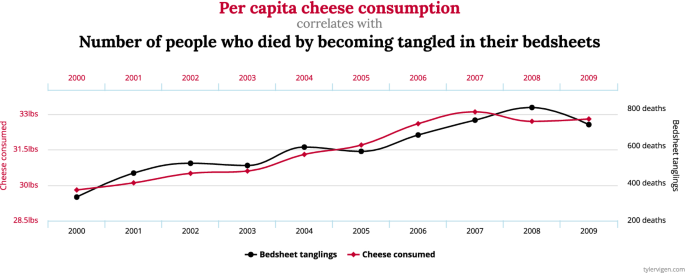

    

    Apparent dependence absurdly indicated by correlation [9]

• Statistical tests: These empirically refute an a priori hypothesis based on existing data. They cannot prove a hypothesis, nor is it correct to form a posterior hypothesis based on the data at hand. Inserting numbers into some formula to verify its correctness is far from being a mathematical proof. However, if the formula is incorrect on a given set of numbers, those numbers make an valid counterexample. It is the same story with statistical tests: the data can be consistent with the test’s hypothesis, but this may be a coincidence. However, when the data is inconsistent with the hypothesis, the data is clearly a counterexample.

  Every (classical) statistical test thus runs along these lines of thinking: suppose that the claim to be verified is a statement $A$.

• a. Formulate a null-hypothesis by negating $A$; let us – in a slight abuse of notation – call the respective opposite claim $\neg A$. The test will be designed to reject $\neg A$ so that the alternative hypothesis, statement $A$, will be assumed (based on the data).

• b. Define a test statistic as some value that:

  (1) Is easy to compute from the data,

  (2) And has a known probability distribution $F( \cdot |\neg A)$ under assumption $\neg A$, i.e., your null-hypothesis.

• c. Given concrete data $D$, compute the test statistic $t_{D}$, and check whether it falls into a certain range of acceptance for the test. This range is typically set as ($1 - \alpha$)-quantile of the distribution of the test statistic’s distribution $F( \cdot |\neg A)$. A popular value to tip the scale between acceptance and rejection of the null-hypothesis is based on the $p$-value, being the $p = { \Pr }(X > t|\neg A)$, i.e., the area under the curve $F(x|\neg A)$ in the interval $\left( {t_{D} ,\infty } \right)$. The null-hypothesis is rejected if $p < 1 - \alpha$, when $\alpha$ is the statistical significance level (usually 95% or something similar).

The dangers of tests applied to big data are thus manifold, and at least include the following sources of error:

• Hypothesis that are formed not a priori, i.e., one seeks to “learn from the data whatever we can learn from it”. The simple truth is: whatever you seek to learn, you will most likely be able to learn it from big data (as much as a conspiracy theoretician will always successfully find secret codes in the bible, or recognize alien landing sites on aerial photos of a landscape).

• Incorrect conclusions from the test’s results: even if the test rejects the null hypothesis, its statistical significance cannot be taken as an error probability, say, in the sense of the $\beta$-reputation as we had above. The usual way of setting up a test is towards controlling the error of first kind, which is the chance of accidentally rejecting the null-hypothesis (although the assumption was correct). This error is complementary to the second type occurring when the null hypothesis is accepted although it is wrong. Controlling the second type of error is much more involved and without deeper considerations, nothing can be said about this other possibility.

Nonetheless, a particularly interesting type of test regards Benford’s Law, which can indicate potential “unnatural” manipulations in data series. This test has seen applications in tax fraud detection and other areas, and is presented here for the intriguing phenomenon that it points out.

3.2 Benford’s Law: Testing for Artificial Data Manipulations

With the battery of statistical tests being widely explored in many branches of computer science, and especially in security, Benford’s law is an exceptional example of a test that, without resorting to specific domains or complicated assumptions, manages to point out manipulations in many different datasets.

The key idea is to test not the numbers for any particular distribution, but rather to look at how the leading digit(s) in the numbers are distributed. Independently, Newcomb [10] (around the year 1881) and later Frank Benford (in 1938) [11], observed that in data arising from natural processes, the digit “1” appears substantially more often as the leading digit. The second most frequent digit is “2”, followed by “3”, with these three making more than 60% of all digits in a dataset.

The Newcomb-Benford law (or Benford law for short) precisely tells $\Pr \left( {{\text{leading digit}}\left( X \right) = d} \right) \propto \log_{10} \frac{d + 1}{d}$ for the digits $d = 1,2, \ldots , 9$, excluding the case of a leading zero for obvious reasons. This formula is surprisingly simple to derive: if $X$ is an $n$-digit real number, when would its first digit be $d$? Obviously only if $d \cdot 10^{n} \le X < \left( {d + 1} \right) \cdot 10^{n}$, or by taking the base-10 logarithm, $\log_{10} \left( d \right) + n \le \log_{10} \left( X \right) \le \log_{10} \left( {d + 1} \right) + n$. The range for the mantissa of ${ \log }\left( X \right)$ to fall within for having $d$ as leading digit has thus the width $\log_{10} \left( {d + 1} \right) - \log_{10} \left( d \right) = \log_{10} \left( {\frac{d + 1}{d}} \right)$. Assuming a “uniform” scattering of numbers over the real line, the claimed likelihoods are obtained. Benford’s originally published material nicely supports the accuracy of this calculation; Fig. 3 shows the empirical values, next to the tabulated values on the right side.

Fig. 3.

Empirical evidence of the Newcomb-Benford law [11]

Testing the law is straightforward: first, compute the relative frequency of leading digits in the given dataset, and compare it to what it should be according to the Newcomb-Benford law above. A deviation exceeding some threshold can be taken as an indication to dig deeper and perhaps look for artificial manipulations to the data (an abnormality). In general, the law is applicable whenever there are (i) many influence factors, (ii) the data set is large (big data). The test will, however, most likely fail on data that (i) is artificial or systematic, such as serial or account numbers, credit card numbers, etc., (ii) the data obeys natural limits (minimum or maximum bound), or (iii) if the data base is small. The exclusion of artificial or systematic data may appear restrictive but only mildly so: Many kinds of numbers like serial numbers, packet indices, network card (MAC) addresses, or ISBN numbers follow a precise structure and are thus often logically checkable for consistency (as they carry check-listed prefixes, verification digits, or similar). Thus, such number, unlike those arising from physical processes, usually do not need a statistical checkup.

The test can be generalized to more than the leading digit, with the respective law following in the same way as in our derivation above. For practical purposes, it is conveniently available in the benford.analysis [12] and BenfordTest [13] packages for the R system [14].

4 Integration Towards Practical Trust Management

Now, let us discuss how the techniques described above lend themselves to application with the signals obtained from technical systems. Anomaly detection and data collection systems can serve as sources for the Bayesian updates and provide data for statistical tests, and Fig. 4 shows how the above trust and manipulation tests would integrate with a system like synERGY: essentially, trust can almost “naturally” be derived from the data that the system generates (note the overlap of Figs. 1 and 4 at the “broker” component), possibly exploiting already existing classification functions that a SIEM or event anomaly detection modules may already offer. The point is here a double use of these features, not only for the system’s primary purpose (e.g., anomaly detection), but also perhaps for trust establishment as an add-on “almost for free” to the existing SIEM. The block “classification” may herein embody not only existing analysis modules from the host system, but also offer its own analyses based on statistics as above.

Fig. 4.

Integration of Trust Models and Manipulation Tests based on the synERGY example

For the NB test, suitable data would include (but be not limited to): latency times, packets per time unit, packet sizes, but in particular also measurement data inside the packet content; basically, any data arising from physical processes would be suitable. Meta-information and protocol overhead data, such as serial numbers, packet numbers, or similar, would not be suitable for NB testing. This data undergoes more systematic checks in anomaly detection engines (where events are analyzed for logical consistency using rule-based checks and by virtue of sophisticated statistics). Basically, the anomaly detection can deliver two kinds of output useable with the Beta reputation model:

• (1) An “everything OK” result upon a test for an anomaly. This would mean that two events in question are being checked for consistency, with a positive outcome, meaning that no indication of suspicious behavior was found. For the component in question, we can compactly represent the trust model as a pair of integers $\left( {a,b} \right)$ being the parameters of the Beta distribution and defining the trust value $\frac{b}{a + b} \in \left( {0,1} \right)$. A Bayesian update on this distribution upon a positive incident then just increases the parameter $b \leftarrow b + 1$ (and accordingly changes the Beta distribution mix if there is uncertainty tied to this update, using model averaging).

• (2) An indication of an anomaly: this would usually refer to some specific component, whose Beta reputation model, represented by a pair $\left( {a,b} \right)$ of parameters for the Beta distribution would be updated into $\left( {a,b} \right) \leftarrow \left( {a + 1,b} \right)$, i.e., increasing the count of negative experience.

5 Conclusion

Whether the analysis of big data is valuable or produces nonsense highly depends on the proper way of data selection and data analytics. This work discussed one application of big data for trust management, and discussed a few do’s and don’ts in the application of some standard and non-standard techniques.

A general word of warning is advisable on the use of black-box models such as some neural networks. Despite the tremendous success of deep learning techniques in a vast variety of applications, the results generally remain confirmed only because they apparently work, but do so without offering any deeper explanations as to the “why”. If not only the result is relevant, but also the reason why it is correct, then neural networks can only deliver half of what is needed. Generally referring to trust, transparency is a qualitative and important requirement, simply because understanding the “why” of a result helps fixing errors and improving mechanisms for the future.

The take-home messages of this work are briefly summarized as follows:

• 1. The strategy on how to fill the gaps in missing data is crucial (you should not infer information that you inserted yourself before).

• 2. You cannot use big data to tell you something (as it can tell you anything); you have to formulate a question and use the big data to get an answer to it.

• 3. Trust is always a subjective matter, no matter how “objective” the underlying model may be. That is, complex math or formalism can create the illusion of accuracy or reliability, although neither may hold.

• 4. Knowing is generally better than not knowing: in a choice between two models, one a white, the other a black box, the more trustworthy model is always white (in security, the trustworthy paradigm is Kerckhoffs’ principle, demanding that every detail of a security algorithm should be openly published, with the security only resting on the secrets being processed).

• 5. Never blindly rely on any machine learning or statistical method: using a black-box model in a default configuration is almost a guarantee of failure. Instead, utilize domain expertise as much as possible, and calibrate/train models as careful as you can. This is the only way of inferring anything decent.

References

Skopik, F., Wurzenberger, M., Fiedler, R.: synERGY: detecting advanced attacks across multiple layers of cyber-physical systems (2018). https://ercim-news.ercim.eu/en114/r-i/synergy-detecting-advanced-attacks-across-multiple-layers-of-cyber-physical-systems. Accessed 13 Jul 2018
SecurityAdvisor. HuemerIT. https://www.huemer-it.com/security-solutions/#SecurityAdvisor. Accessed 4 July 2018
Wurzenberger, M., Skopik, F., Settanni, G., et al.: AECID: a self-learning anomaly detection approach based on light-weight log parser models. In: Proceedings of the 4th International Conference on Information Systems Security and Privacy, pp. 386–397. SCITEPRESS - Science and Technology Publications (2018)
Friedberg, I., Skopik, F., Settanni, G., et al.: Combating advanced persistent threats: from network event correlation to incident detection. Comput. Secur. 48, 35–57 (2015). https://doi.org/10.1016/j.cose.2014.09.006
Rass, S., Kurowski, S.: On Bayesian trust and risk forecasting for compound systems. In: Proceedings of the 7th International Conference on IT Security Incident Management & IT Forensics (IMF), pp. 69–82. IEEE Computer Society (2013)
Robert, C.P.: The Bayesian Choice. Springer, New York (2001)
Jøsang, A., Ismail, R.: The beta reputation system. In: Proceedings of the 15th Bled Electronic Commerce Conference (2002)
Rass, S., Slamanig, D.: Cryptography for Security and Privacy in Cloud Computing. Artech House, Norwood (2013)
Vigen, T.: Spurious Correlations, 1st edn. Hachette Books, New York (2015)
Newcomb, S.: Note on the frequency of use of the different digits in natural numbers. Am. J. Math. 4(1/4), 39 (1881). https://doi.org/10.2307/2369148
Benford, F.: The law of anomalous numbers. Proc. Am. Philos. Soc. 78(4), 551–572 (1938)
Cinelli, C.: benford.analysis: Benford analysis for data validation and forensic analytics (2017). https://CRAN.R-project.org/package=benford.analysis
Joenssen, D.W.: BenfordTests: statistical tests for evaluating conformity to Benford’s Law (2015). https://CRAN.R-project.org/package=BenfordTests
R Core Team. R: a language and environment for statistical computing (2018). http://www.R-project.org
Acknowledgement
This work was partly funded by the Austrian FFG research project synERGY (855457).
Author information
Authors and Affiliations
Corresponding author
Editor information
Editors and Affiliations
Rights and permissions
Copyright information
© 2019 IFIP International Federation for Information Processing
About this chapter
Cite this chapter
Rass, S., Schorn, A., Skopik, F. (2019). Trust and Distrust: On Sense and Nonsense in Big Data. In: Kosta, E., Pierson, J., Slamanig, D., Fischer-Hübner, S., Krenn, S. (eds) Privacy and Identity Management. Fairness, Accountability, and Transparency in the Age of Big Data. Privacy and Identity 2018. IFIP Advances in Information and Communication Technology(), vol 547. Springer, Cham. https://doi.org/10.1007/978-3-030-16744-8_6
Download citation
DOI: https://doi.org/10.1007/978-3-030-16744-8_6
Published:
Publisher Name: Springer, Cham
Print ISBN: 978-3-030-16743-1
Online ISBN: 978-3-030-16744-8
eBook Packages: Computer ScienceComputer Science (R0)