
Abstract
A factor is an independent variable. A factorial design completely crosses two or more factors. It is an efficient design that simultaneously studies main effects of factors and their interactions. A distinction is made between factors that can be manipulated by researchers and factors that cannot be manipulated. Usually, the effects of manipulable factors are causally interpreted. Nonmanipulable factors are included for two different reasons, but they should not be dichotomized. First, to increase the precision of parameter estimates and the power of statistical tests. The nonmanipulable factor is included as a blocking variable in a randomized block design (if its values are known before participants are assigned to conditions) or as a covariate in the analysis of the data. Second, to study their relations with manipulable factors, but these relations should not be causally interpreted. The statistical analysis of factorial design data has to be tuned to the type of dependent variable (DV). Usually, ANOVA or ANCOVA are applied to (approximately) continuous DVs, but these methods make strong assumptions. Akritas et al.’s (J Am Stat Assoc 92:3375–3384, 1997) nonparametric method is more appropriate to analyze (approximately) continuous and ranked DVs. The preferred methods for dichotomous, nominal-categorical, and ordinal-categorical DVs are the logit, baseline-category, and cumulative logit models, respectively. Often, researchers apply omnibus statistical tests to factorial design data. These tests mainly fit into exploratory research. Confirmatory studies prespecify specific hypotheses. The proper methods to test these hypotheses are planned comparisons of conditions.
Keywords
- Baseline splitting
- Cumulative splitting
- Dichotomization
- Factorial design
- Interaction effect
- Linear contrast
- Logit model
- Main effect
- Manipulable and nonmanipulable factors
- Planned comparisons
The previous chapters focused on the situation where the effect of one independent variable (IV) on a dependent variable (DV) is studied. For example, the effect of a new psychotherapy compared to the standard therapy (IV: Treatment) on patients’ depression test score (DV: depressive mood). This chapter is directed to research situations that involve more than one IV. The inclusion of several IVs into one design has some advantages, but also a disadvantage. The simultaneous study of several IVs is usually more efficient and less expensive than separate studies of each of the IVs. Moreover, the simultaneous study of different IVs yields more information than separate studies because interactions can be studied. However, the number of different combinations of IVs might become very large and unmanageable.
The discussion is restricted to between-subjects designs with completely crossed factors. This situation suffices to show some common errors and to discuss methods to prevent or correct them.
18.1 Factorial Designs
The situation is considered of research designs that have two or more IVs. In the context of research designs, an IV is called a factor and the values of the IV the levels of the factor . For example, a dichotomous IV that consists of a new and a standard treatment is called a treatment factor with two levels.
A factorial design is a design that uses two or more factors that are combined. The complete crossing of factors means that each level of a factor is combined with each level of the other factors. Each of these combinations is called a cell of the factorial design . Participants of the study are distributed across the cells and data are collected for each cell of the design. Example 18.1 clarifies this terminology.
Example 18.1 A completely crossed 2 × 2 factorial design
A treatment factor has two levels: a new treatment and the standard treatment. The duration factor also has two levels: each of the two treatments is applied 10 or 20 weeks. The complete crossing of the two factors yields 2 (treatments) × 2 (durations) = 4 cells of the design:
Duration factor | |||
|---|---|---|---|
10 weeks (short) | 20 weeks (long) | ||
Treatment factor | New | × | × |
Standard | × | × | |
A cross means that participants are assigned to the cell, and data are collected. For example, 25 participants are assigned to each of the four cells, and a test is administered to each of the 4 (cells) × 25 (participants) = 100 participants. The design is called a 2 × 2 factorial design because the first factor (Treatment) has two levels and the second factor (Duration) has two levels.
The design of Example 18.1 is the simplest possible factorial design because it has two factors and two levels per factor. The factorial design can be extended to designs with more than two factors and more than two levels per factor. For example, a design with three factors (A, B, and C), where Factor A has two levels, Factor B three levels, and Factor C four levels has 2 × 3 × 4 = 24 cells, and is called a 2 × 3 × 4 factorial design. The number of cells increases with the number of factors and the number of levels per factors. Therefore, a design with many factors and many levels per factor easily becomes unmanageable in practice.
An important distinction is between manipulable and nonmanipulable factors. A manipulable factor is an IV that can be manipulated by researchers, whereas a nonmanipulable factor cannot be manipulated (cf. Sect. 4.1 of this book). Examples of manipulable factors are the Treatment and Duration factors of Example 18.1. Examples of nonmanipulable factors are Age, Gender, Income, Educational Level, and Socioeconomic Status (SES). This distinction is relevant for the interpretation of the results of a study because manipulable and nonmanipulable factors have a different status within factorial designs (see Sect. 18.4 of this chapter).
18.2 Main and Interaction Effects
A factorial design admits the study of the main and interaction effects of the factors. A main effect is the differential effect of the levels of a factor on the DV, whereas an interaction effect is the differential effects of combinations of levels of factors on the DV. Main effects can be studied by doing separate studies on each of the factors, but interaction effects can only be studied by combining levels of different factors into one study. Example 18.2 illustrates the concepts of main and interaction effects.
Example 18.2 Main and interaction effects on a test score DV, 2 × 2 factorial design (constructed data)
A sample of 100 depressive patients is selected for a study. The patients are randomly assigned to the four conditions of the 2 × 2 factorial design of Example 18.1 (25 patients per cell of the design). After completing the treatment, a depression test is administered to each of the patients. The test has 30 items and each of the items has five answer categories that are integer scored (i.e., 1, 2, 3, 4, or 5). The test score is the sum of the 30 item scores. The minimum possible test score is Xmin = 30 × 1 = 30 (a score of 1 at each of the 30 items), and the maximum possible score is Xmax = 30 × 5 = 150 (a score of 5 at each of the 30 items). Moreover, after completing the treatment, each of the patients is interviewed by a clinical psychologist. The psychologist evaluates patients’ depressive mood. This example discusses main and interaction effects on an approximately continuous DV (i.e., the depression test score), while Examples 18.5 through 18.7 discuss these effects on other types of DVs. The following effects are distinguished:
-
(1)
A main effect of the treatment factor, and no main effect of the duration factor, and no interaction effect;
-
(2)
a main effect of the duration factor, and no main effect of the treatment factor, and no interaction effect;
-
(3)
main effects of both treatment and duration factors, but no interaction effect;
-
(4)
an ordinal interaction effect;
-
(5)
a disordinal interaction effect.
These effects are demonstrated using the (fictitious) means of the depression test scores. The mean scores of the four cells are indicated by XNS (new treatment/short (10 weeks duration)), XNL (new treatment/long (20 weeks duration)), XSS (standard treatment/short (10 weeks duration)), and XSL (standard treatment/long (20 weeks duration)). Idealized versions of the five types of effects are given.
-
(1)
Only a main effect of the treatment: \( \bar{X}_{NS} = \bar{X}_{NL} = 50 \), and \( \bar{X}_{SS} = \bar{X}_{SL} = 90 \) (see Fig. 18.1).
Fig. 18.1 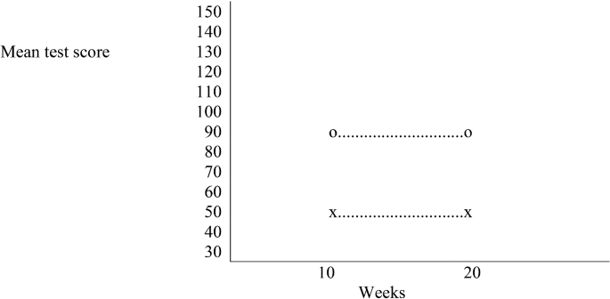
Only a main effect of the treatment. A cross indicates the new treatment and a circle the standard treatment
A dotted line connects the crosses and the circles, respectively. The lines are parallel, which means that the treatment effect is the same for each of the two levels (i.e., 10 and 20 weeks) of the duration factor: the new treatment decreases the depression test score at each of the two levels of the duration factor.
-
(2)
Only a main effect of the duration: \( \bar{X}_{NS} = \bar{X}_{SS} = 80 \), and \( \bar{X}_{NL} = \bar{X}_{SL} = 60 \) (see Fig. 18.2).
Fig. 18.2 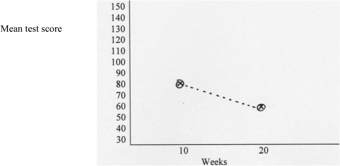
Only a main effect of duration. A cross indicates the new treatment and a circle the standard treatment
The dotted lines that connect the crosses and circles, respectively, coincide, which means that the duration effect is the same for each of the two levels (new and standard) of the treatment factor: the 20-weeks duration decreases the depression test score at each of the two levels of the treatment factor.
-
(3)
A main effect of both treatment and duration: \( \bar{X}_{NS} = 70 \), \( \bar{X}_{NL} = 50 \), \( \bar{X}_{SS} = 100 \), and \( \bar{X}_{SL} = 80 \) (see Fig. 18.3).
Fig. 18.3 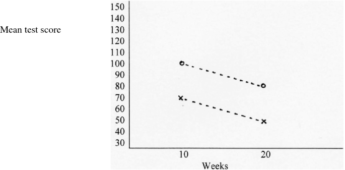
A main effect of both treatment and duration. A cross indicates the new treatment and a circle the standard treatment
The figure shows that the new treatment and the 20-weeks duration decreases the test score. Moreover, the difference between the 10 and 20 weeks durations (i.e., 20 score points) is the same for each of the two treatments, and the difference between the standard and new treatments (i.e., 30 score points) is the same for each of the two durations.
-
(4)
An ordinal interaction effect : \( \bar{X}_{NS} = 50 \), \( \bar{X}_{SS} = 60 \), \( \left| {\bar{X}_{NL} = 40} \right. \), and \( \bar{X}_{SL} = 80 \) (see Fig. 18.4).
Fig. 18.4 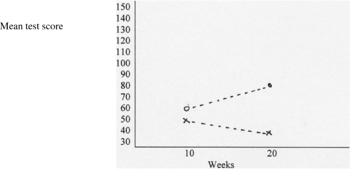
An ordinal interaction effect. A cross indicates the new treatment and a circle the standard treatment
The figure shows the interaction effect: the difference between the standard and new treatment is larger for the 20 weeks duration (i.e., 40 score points) than for the 10 weeks duration (i.e., 10 score points). This type of interaction was called ordinal by Bracht and Glass (1968) because the mean of the new treatment is smaller than the mean of the standard treatment for both durations.
-
(5)
A disordinal interaction effect : \( \bar{X}_{NS} = 60 \), \( \bar{X}_{SS} = 90 \), \( \bar{X}_{NL} = 90 \), and \( \bar{X}_{SL} = 60 \) (see Fig. 18.5).
Fig. 18.5 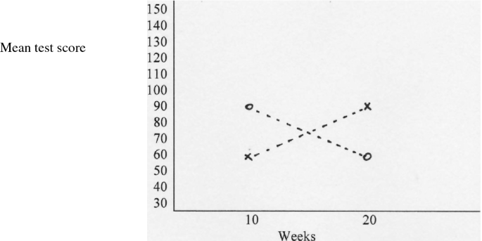
A disordinal interaction effect. A cross indicates the new treatment and a circle the standard treatment


The figure shows the interaction effect: the mean of the new treatment is smaller than the mean of the standard treatment when the duration is 10 weeks, but the mean of the new treatment is larger than the mean of the standard treatment when the duration is 20 weeks. This type of interaction was called disordinal by Bracht and Glass (1968).
The example demonstrates some properties of factorial designs. It gives cause to the following comments.
First, a factorial design combines two or more factors and admits the study of main effects and their interactions. The main effects could be studied by doing separate studies on each of the factors (see Example 18.3).
Example 18.3 Separate studies on the effects of the two factors of Example 18.2
Two separate studies are done on the treatment and duration effects. The first study is on the effect of the treatment. A sample of 50 patients is selected, 25 of them are randomly assigned to 20 weeks new treatment and the other 25 to 20 weeks standard treatment. The second is on the duration effect, and is done with the treatment that had the best results in the first study. For example, if in the first study, the new treatment decreased the depression test scores more than the standard treatment, the new treatment is selected for the second study. A new sample of 50 patients is selected, 25 of them are randomly assigned to the 20-weeks version of the new treatment and the other 25 to the 10-weeks version. The first study assesses the effect of the 20-weeks version of the new treatment, and the second study compares the 20- and 10-weeks versions of the new treatment. However, the two studies do not yield information on the interaction of the treatment and duration factors. In contrast, the 2 × 2 factorial design of Example 18.2 yields information on the effects of the two factors as well as their interaction.
Second, the interpretation of main effects is not straightforward when interactions are present. For example, the dotted lines of Figs. 18.1, 18.2, and 18.3 are parallel or coincide, which means that interaction is absent. Therefore, the interpretation of the main effects is straightforward, for example, Fig. 18.1 shows that the new treatment is more effective than the standard treatment, and that the effect is the same for the 10- and 20-weeks versions. The dotted lines of Figs. 18.4 and 18.5 are not parallel, which means that the factors interact. Therefore, the interpretation of one factor depends on the other factor, for example, Fig. 18.5 shows that the 10-weeks version of the new treatment is more effective than the 10-weeks version of the standard treatment, but that the 20-weeks version of the new treatment is less effective than the 20-weeks version of the standard treatment.
Third, the distinction between ordinal and disordinal interactions is relevant for the interpretation of the results of a factorial design. The dotted lines of an ordinal interaction do not cross (see Fig. 18.4), whereas the dotted lines of a disordinal interaction cross (see Fig. 18.5). The interpretation of an ordinal interaction is simpler than the interpretation of a disordinal interaction. For example, the ordinal interaction of Fig. 18.4 implies that the new treatment always has to be preferred above the standard treatment because the new treatment yields smaller depression test scores for both the 10- and 20-weeks durations. The interpretation of a disordinal interaction is more complex. For example, the disordinal interaction of Fig. 18.5 shows that the new treatment has to be preferred if the duration is 10 weeks, but the standard treatment has to be preferred if the duration is 20 weeks.
18.3 Testing Main and Interaction Effects
The figures of the previous section are idealized pictures of effects. Usually, empirical data show less clear effects, and statistical methods are needed to test effects. Section 11.2 of this book distinguished five types of variables: (1) dichotomous, (2) nominal-categorical, (3) ordinal-categorical, (4) ranked, and (5) continuous variables. This section discusses factorial designs that have different types of DVs.
18.3.1 Continuous and Ranked DVs
The conventional method to analyze factorial design data is Analysis of Variance (ANOVA). ANOVA is applied to continuous DVs, such as, reaction times, and also to DVs that are approximately continuous, such as, test scores. Conventional ANOVA assumes that (1) the DV is normally distributed in each cell of the design, and (2) the variances of the DV are homogeneous (i.e., the same in each cell of the design). It follows from these assumptions that only the means of the DV can vary between cells of the design.
The ANOVA assumptions are rather strict, and are easily violated in empirical data. It is known for a long time that violations of ANOVA assumptions can increase Type I and II errors of ANOVA tests (Clinch & Kesselman, 1982; Glass, Peckham, & Sanders, 1972). Nonparametric alternatives of parametric ANOVA tests were developed. Toothaker and Newman (1994) studied the performance of three nonparametric tests (i.e., the Puri and Sen, rank transform, and aligned rank tests). These tests do not make the normality assumption, but assume that the distribution of the DV is the same in each cell of the design except for its location. This assumption is also very strong, and is also easily violated in empirical data. Toothaker and Newman (1994) simulated data for 2 × 2, 2 × 4, and 4 × 4 factorial designs. Their results show that the three nonparametric tests can increase the Type I and II errors of the tests.
Akritas, Arnold, and Brunner (1997) developed another nonparametric method for the analysis of factorial design data. As other nonparametric methods, their method uses the rank numbers of the DV scores. However, in contrast to other nonparametric methods, it does not make the equality of distributions assumption. Theoretically, the method is well-suited for the analysis of factorial design data. The method can test main and interaction effects, does not make strong assumptions, and can be applied to designs that have different numbers of participants per cell of the design. Moreover, the method is less sensitive to outliers than conventional ANOVA because it is based on rank numbers (see Chap. 17 of this book). Example 18.4 illustrates how to handle the data of the 2 × 2 factorial design of Example 18.2.
Example 18.4 Ranking data of the 2 × 2 factorial design of Example 18.2
The test scores of the 100 patients of Example 18.2 are pooled, and rank numbers are assigned to these scores. Ties are handled by the midranks method (see Sect. 11.4.10 of this book). Null hypotheses on main and interaction effects are tested using statistics that are reported by Akritas et al. (1997). Wilcox (2012, Sect. 7.9.1) gives an R function for doing the computations.
It is tempting to apply a two-step procedure. In the first step, the homogeneity of variance null hypothesis is tested. In the second step, a choice is made between conventional ANOVA and Akritas et al.’s method: ANOVA is applied if the null hypothesis of homogeneous variance is not rejected, and Akritas et al.’s method is applied if this null hypothesis is rejected. However, it is known that a two-step procedure for testing the difference between two means increases the Type I error of the testing procedure (see Sect. 12.3 of this book). Therefore, it is conjectured that a two-step procedure for testing factorial design data will have negative effects on the Type I error. For the time being, the Akritas et al.’s method is the recommended method to test effects of factorial designs that have (approximately) continuous or ranked DV scores.
18.3.2 Dichotomous DVs
Akritas et al.’s method is appropriate for (approximately) continuous and ranked DV scores, but cannot be applied to dichotomous, nominal-categorical, and ordinal-categorical DV scores. These types of scores have to be analyzed with logit models (Agresti, 2002).
A dichotomous DV consists of two categories, that is, a first and a second category, for example, the first category is ‘passed the examination’ and the second category is ‘failed the examination’. The data are the frequencies of these two categories, for example, the frequency of students who passed the examination and the frequency of students who failed. The odds of the two categories is the ratio of these two frequencies (see Sect. 11.4.1 of this book):
The logit of two categories is the natural logarithm (i.e., logarithm at base e = 2.718…) of the odds:
where ln denotes the natural logarithm.
The data of a factorial design that has a dichotomous DV are the frequencies of the two categories per cell of the design. Using Eq. 18.2 these frequencies are transformed to logits per cell of the design. The logits are analyzed by logit models. A logit model is used to test main and interaction effects of factorial designs that have a dichotomous DV. The logit model analysis resembles ANOVA in the sense that both methods test null hypothesis on main and interaction effects. However, the logit model applies to dichotomous DVs, whereas ANOVA applies to continuous DVs. Moreover, the logit model makes less stringent assumptions than ANOVA. Example 18.5 demonstrates how the logit model is applied to analyze a dichotomous DV of the 2 × 2 factorial design of Example 18.2.
Example 18.5 The 2 × 2 factorial design of Example 18.2 and a dichotomous DV
A cutting score is defined on the depression test scores of Example 18.2. For each of the 100 patients it is checked whether his (her) test score is below or above the cutting score: patients who have a test score equal to or below the cutting score are labeled ‘sufficiently recovered’ and patients who have a test score above the cutting score are labeled ‘not sufficiently recovered’. The cutting score splits the test scores into a dichotomous variable with two categories (i.e., sufficiently and not sufficiently recovered). The fictitious frequencies per cell of the 2 × 2 factorial design are:
Weeks | |||
|---|---|---|---|
10 | 20 | ||
Treatment | New | Rec.: 22 | Rec.: 22 |
Not rec.: 3 | Not rec.: 3 | ||
Logit: 1.99 | Logit: 1.99 | ||
Standard | Rec.: 14 | Rec.: 14 | |
Not rec.: 11 | Not rec.: 11 | ||
Logit: 0.24 | Logit: 0.24 | ||
The table reports the frequencies of sufficiently recovered (Rec.) and not sufficiently recovered (Not rec.) patients and the logit transformation per cell of the design. For example, 25 patients were assigned to the 10-weeks version of the new treatment, 22 of them were sufficiently recovered and 3 were not sufficiently recovered. It follows from Eq. 18.2 that the logit is:
Figure 18.6 gives the graphical representation of the logits.

Only a main effect of the treatment. A cross indicates the new treatment and a circle the standard treatment
The logit model is used to test null hypotheses on main and interaction effects. Figure 18.6 is the idealized picture of only a main effect of the treatment factor on the logits. Figure 18.6 is comparable to Fig. 18.1 of Sect. 18.2. Figure 18.1 shows the main effect of the treatment factor on the test scores, while Fig. 18.6 shows the main effect of the treatment factor on the dichotomized test scores. Both figures give an idealized picture of the main effect of the treatment factor in absence of the main effect of the duration factor and the treatment × duration interaction. The figures of the other effects (only a duration main effect, a treatment and duration main effect, an ordinal treatment × duration interaction effect, and a disordinal treatment × duration interaction effect) on the dichotomous scores yield idealized pictures that are comparable to Figs. 18.2, 18.3, 18.4, and 18.5, respectively.
18.3.3 Nominal-Categorical DVs
The logit model is also appropriate for the analysis of factorial designs that have categorical DVs. A nominal-categorical DV is handled by conceptually splitting it into dichotomous variables, which combine a base line category with each of the other categories, and simultaneously applying the logit model to these dichotomous variables (Agresti, 2002, Sect. 7.1).
Example 18.6 demonstrates how the logit model is applied to a nominal-categorical DV of the 2 × 2 factorial design of Example 18.2.
Example 18.6 The 2 × 2 Factorial design of Example 18.2 and a nominal-categorical DV
The 100 patients of Example 18.2 were interviewed by a clinical psychologist. The psychologist evaluated each of the patients using a nominal and an ordinal scale. The nominal scale is described in this example, and the ordinal scale in Example 18.7 of the following section. The nominal scale has three categories: the patient feels (1) relaxed, (2) fatigued, and (3) stressed. The nominal variable is conceptually split into two dichotomous variables. The relaxed category is taken as the baseline category, and each of the other two categories is combined with the baseline category. Figure 18.7 shows the baseline splitting of the three-category nominal scale.

Baseline-splitting of a three-category nominal variable into two dichotomous variables
The psychologist assigned each of the 100 patients to one of the three categories, and the category frequencies are counted per cell of the 2 × 2 factorial design. Conceptually, the three-category variable is split into two dichotomous variables that preserve the nominal nature of the three categories. As an example, Fig. 18.8 shows the fictitious frequencies of the three-category variable, and the frequencies of the two dichotomous variables for the 10-weeks version of the new treatment.

Fictitious frequencies three-category variable and its baseline splittings, 10-weeks version of the new treatment
The logit model is appropriate to analyze the frequencies of the two dichotomous variables. Although it seems plausible, it is not allowed to apply the logit model separately to each of the two dichotomous variables because these two variables are dependent. For example, the dichotomous variables of Fig. 18.8a and b are dependent because the same 13 relaxed patients are included into each of the two dichotomous variables. The baseline-category logit model is a method that simultaneously analyzes the two dichotomous variables (Agresti, 2002, Sect. 7.1). The model tests null hypotheses on the main and interaction effects of factorial designs.
Example 18.6 demonstrated baseline-splitting of a three-category nominal variable. Similarly, nominal variables that have more than three categories can conceptually be split into dichotomous variables, and the baseline-category logit model can be applied to test null hypotheses on main and interaction effects.
18.3.4 Ordinal-Categorical DVs
The logit model is also suited for the analysis of ordinal-categorical DVs. However, the splitting of an ordinal-categorical variable differs from the splitting of a nominal-categorical variable. An ordinal-categorical DV is handled by conceptually splitting it into dichotomous variables that preserve the order of the categories (Agresti, 2002, Sect. 7.2). Example 18.7 demonstrates how the logit model is applied to an ordinal-categorical DV of the 2 × 2 factorial design of Example 18.2.
Example 18.7 The 2 × 2 factorial design of Example 18.2 and an ordinal-categorical DV
In addition to the nominal scale (see Example 18.6), the psychologist used an ordinal scale to assess the severity of patients’ depression. The scale has three ordered categories: (1) not depressed, (2) moderately depressed, and (3) strongly depressed. The ordinal variable is conceptually split into two dichotomous variables that preserve the order of the three categories. Three ways of splitting preserve the ordinal nature of a variable, but only cumulative splitting (Agresti, 2002, Sect. 7.2) is discussed in this chapter. For the other two splittings (i.e., adjacent-categories and continuation-ratio splitting) the reader is referred to, among others, Agresti (2002, Sect. 7.2). Figure 18.9 shows the cumulative splitting of the ordinal three-category variable.

Cumulative splitting of a three-category ordinal variable into two dichotomous variables
The dichotomous variable of Fig. 18.9a combines the moderately and not depressed categories, while the dichotomous variable of Fig. 18.9b combines the strongly and moderately depressed categories. The psychologist assigned each of the 100 patients to one of the three ordered categories, and the category frequencies are counted per cell of the 2 × 2 factorial design. Conceptually, the three-category variable is split into two dichotomous variables that preserve the ordinal nature of the three categories. As an example, Fig. 18.10 shows the fictitious frequencies of the two dichotomous variables for the 10-weeks version of the new treatment.

Fictitious frequencies three-category variable and its cumulative splitting, 10-weeks version of the new treatment
The logit model is suited to analyze the frequencies of the two dichotomous variables. It is not allowed to apply the logit model separately to each of the two dichotomous variables because these two variables are dependent. For example, the two dichotomous variables of Fig. 18.10 are dependent because the same 15 not depressed patients are counted in each of the two dichotomous variables. The cumulative logit model is a method that simultaneously analyzes the two dichotomous variables (Agresti, 2002, Sect. 7.2). The model tests null hypotheses on the main and interaction effects of factorial designs.
Example 18.7 demonstrated cumulative splitting of a three-category ordinal variable. In the same way, ordinal variables that have more than three categories can conceptually be split into dichotomous variables, and the cumulative logit model can be applied to test null hypotheses on main and interaction effects of factorial designs.
The logit model is the appropriate method for the analysis of dichotomous and nominal- and ordinal-categorical DVs. The interpretation of the effects of the factors of a factorial design on a dichotomous variable is straightforward. The main and interaction effects are on the logits of a dichotomous variable (see Fig. 18.6), and the interpretation is similar to the interpretation of the effects of factors on a continuous variable (cf. Figs. 18.1 and 18.6). However, the interpretation of the effects of factors on nominal- and ordinal-categorical DVs is less straightforward. The effects are in logits, but factors influence more than one dichotomous variable. For example, the effects of the factors of the 2 × 2 design of Example 18.2 on three-category DVs is on two dependent dichotomous variables (see Examples 18.6 and 18.7).
In the practice of behavioral research, it is rather common to score the ordered categories of a DV by assigning rank numbers to the categories, for example, the three ordered categories of the DV of Example 18.7 are scored: 1 for not depressed, 2 for moderately depressed, and 3 for strongly depressed. Subsequently, conventional ANOVA is applied to these scores. The ANOVA-assumptions (i.e., a normally distributed DV with homogeneous variance per cell of the design) are almost surely violated, which can increase Type I and II errors of statistical tests. It is advised against integer scoring of ordered categories, and it is recommended to apply the cumulative logit model to analyze ordinal-categorical DV’s.
18.4 Nonmanipulable Factors
A nonmanipulable factor is an IV that cannot be manipulated by researchers, whereas a manipulable factor is an IV that can be manipulated. Examples, of nonmanipulable factors are Gender, Age, Educational level, and SES. The complete combination of manipulable and nonmanipulable factors yields a design that is similar to a factorial design (see Example 18.8).
Example 18.8 Combining a manipulable and a nonmanipulable factor
A study is planned on the effects of a new arithmetic course compared to the standard course. A sample of students is selected, half of them are randomly assigned to the new course and the other half to the standard course. Moreover, the researchers include the nonmanipulable gender factor into the design. The arithmetic performance of each of the students is measured at the end of the course with a 30-item arithmetic test. Combining the manipulable course factor with the nonmanipulable gender factor yields a design that is similar to a 2 × 2 factorial design:
Gender | |||
|---|---|---|---|
Boys | Girls | ||
Course | New | × | × |
Standard | × | × | |
A cross means that students are present in the cell of the design, and the arithmetic test is administered to them.
The designs of Examples 18.1 and 18.8 are of similar structure. Both designs have two factors with two levels, which yield four different combinations. However, the designs differ in an important aspect. The two factors of Example 18.1 (i.e., Treatment and Duration) are manipulable, whereas one factor of Example 18.8 (i.e., Course) is manipulable and the other factor (i.e., Gender) is not manipulable. Nonmanipulable variables are included into designs for two different reasons. First, to increase the precision of parameter estimates and the power of statistical tests, and, second, to study their relations with manipulable factors.
Nonmanipulable variables are included as blocking variables or covariates. Section 4.5.1 of this book discussed blocking variables and Sect. 4.5.2 covariates. Blocking variables and covariates increase the precision of parameter estimates and the power of statistical tests. It is required that the blocking variable or covariate is associated with the DV, and the variability of the DV is sufficiently smaller within blocks or covariate values than between blocks or covariate values. Moreover, it is required that the manipulable factors do not affect blocking variables or covariates.
A nonmanipulable variable can only be used as a blocking variable if its values are known to the researchers before participants are assigned to conditions. The resulting design is a randomized block design (see Sect. 4.5.1 of this book). Example 18.9 demonstrates the use of Gender as a blocking variable in the design of Example 18.8.
Example 18.9 A nonmanipulable blocking variable to increase precision
The sample of students of Example 18.8 is divided into subsamples of boys and girls. Half of the number of boys is randomly assigned to the new arithmetic course and the other half to the standard course. Moreover, half of the number of girls is randomly assigned to the new course and the other half to the standard course. The design of this example is a randomized block design (see Sect. 4.5.1 of this book).
A nonmanipulable factor may also be included as a covariate. The covariate does not need to be measured before participants are assigned to the conditions of the study. The covariate can be measured at any time of the study, as long as the manipulable factors do not affect the covariate. Example 18.10 demonstrates the use of Gender as a covariate.
Example 18.10 A nonmanipulable covariate to increase precision
Half of the number of students of Example 18.8 is randomly assigned to the new course and the other half to the standard course. At the end of the course the arithmetic test is administered to each of the students, and the gender of each student is registered. The manipulable course factor cannot affect students’ gender. Therefore, Gender is a covariate that can be used in the statistical analysis of the data.
Examples 18.9 and 18.10 demonstrate a difference between a blocking variable and a covariate. A blocking variable has to be used before participants are assigned to conditions. Therefore, researchers have control over the distribution of the nonmanipulable variable across the conditions. For example, Example 18.9 assigns 50% of the boys and 50% of the girls to the new course, and 50% of the boys and 50% of the girls to the standard course. In contrast, a covariate can be measured before and after participants are assigned to conditions. If a covariate is measured after participants are assigned to conditions, researchers have no control over the distribution of the nonmanipulable variable across conditions. For example, in the design of Example 18.10 it is not known in advance how many boys and how many girls will participate in the new course, and how many boys and how many girls will participate in the standard course.
A nonmanipulable factor needs not only be included to increase precision, but may be of interest of its own. Researchers may include a nonmanipulable factor in a design because they are interested in the association between the nonmanipulable and the manipulable factors (see Example 18.11).
Example 18.11 A nonmanipulable variable of interest
The nonmanipulable gender factor of Example 18.8 is included because researchers are interested in the relation of Gender with the course factor. For example, researchers hypothesize that the new course has more effect on the arithmetic test scores of girls than boys. This hypothesis is on the Course × Gender interaction. The difference between the test scores of new and standard course girls is larger than the difference between new and standard course boys.
The interpretation of nonmanipulable and manipulable factors differs. Usually, a causal interpretation is given of the effect of a manipulable variable on a DV. For example, effects of the manipulable treatment and duration factors of Example 18.2 are interpreted as caused by these factors. The causal interpretation is based on the random assignment of participants to the levels of manipulable factors, which controls selection bias (see Sect. 4.4 of this book). However, participants cannot be randomly assigned to the levels of a nonmanipulable factor, such as, gender. Therefore, the interpretation of nonmanipulable factors has to be in terms of association instead of causation (see Sect. 4.2 of this book) because other variables may cause the effects (see Example 18.12).
Example 18.12 The interpretation of an interaction hypothesis
A study is done to test the Course × Gender interaction hypothesis of Example 18.11. The study supports an interaction effect: the difference in arithmetic test scores of the new and standard course groups is larger for girls than for boys. The study shows that Gender is related to Course, but this relation does not imply that Gender causes the interaction effect because other variables may cause the interaction. For example, students’ arithmetic skill may cause the interaction: more skilled students profit more from the new course than less skilled students, and the girls of the study are more skilled than the boys.
Most of the statistical methods for the analysis of factorial design data can handle blocking variables and covariates. Usually, ANOVA is applied to analyze data from randomized block designs, and Analysis of Covariance (ANCOVA) to analyze data of factorial designs that include a covariate. These methods apply to (approximately) continuous DVs and make strong assumptions. Akritas et al.’s (1997) method makes less stringent assumptions and is applicable to continuous and ranked DVs of randomized block designs. Blocking variables and covariates can be included in logit models for the analysis of dichotomous, nominal-categorical, and ordinal-categorical DVs of factorial designs. Finally, nonmanipulable factors that are included because of their own interest can be analyzed by correlational methods.
18.5 Dichotomization of Nonmanipulable Independent Variables
In general, factors have a limited number of levels, for example, a factor that has two experimental and one control condition has three levels. Nonmanipulable IVs may have large numbers of values, for example, age in years and IQ have a broad range of different values. Some researchers dichotomize continuous and test score IVs. The IV is split into two groups of participants, for example, aged below and above the sample median age, and IQs below and above the sample mean IQ. In this way they create a factor that has few levels (e.g., younger and older participants), and about equal numbers of participants per level (e.g., 50% participants younger than the median age, and 50% older than the median). This practice was adopted in the pre-computer era to decrease the computational burden, but continues. For example, MacCallum, Zhand, Preacher, and Rucker (2002) examined articles published in the Journal of Personality and Social Psychology, Journal of Consulting and Clinical Psychology, and Journal of Counseling Psychology in 1998, 1999, and 2000. They found that 11.5% of these articles reported dichotomization of one or more variables.
This practice was criticized by Humphreys and Fleishman (1974) and Cohen (1983). Allison, Gorman, and Primeva (1993) recommended not to dichotomize continuous IVs, and this recommendation was supported by a literature review of MacCallum et al. (2002). Usually, the consequences of dichotomization are negative. First, information is lost. For example, if IQs are dichotomized into IQs equal to and larger than 100 and IQs smaller than 100, the IQ differences within each of these two categories is lost, for example, no difference is made between IQs of 100 and 130 because both IQs belong to the higher IQ category. Second, the effect size and the power of statistical tests may decrease. Third, if two variables are dichotomized, spurious significant results and overestimated effect sizes may occur. Fourth, it is impossible to detect nonlinear relations between a dichotomized IV and the DV. Finally, the reliability of the IV may decrease by dichotomization.
DeCoster, Iselin, and Galucci (2009) generally confirmed these results, but slightly nuanced them. A dichotomized IV may perform as well as the undichotomized IV under strict conditions. However, these conditions are hard to fulfill in practice. The general conclusion is therefore that dichotomization of continuous and test score DVs is not recommended. Moreover, dichotomization is nowadays superfluous because most methods for the analysis of factorial design data can cope with nonmanipulable IVs without dichotomization.
18.6 Testing Specific Substantive Hypotheses
The tests of the previous sections are omnibus tests of main and interaction effects. For example, if a factor has two experimental (E1- and E2-) and one control (C-) condition, the F-test of an ANOVA tests the null hypothesis that the three DV-means are equal:
If this null hypothesis is rejected, it is likely that the three means differ. However, the test of null hypothesis Eq. 18.3 is an omnibus test that does not tell which of the means differ from each other: (1) μE1 and μE2, (2) μE1 and μC, or (3) μE2 and μC. This information is obtained by applying pairwise comparisons of the means. A large number of methods were developed to compare pairs of means (Jaccard, Becker, & Wood, 1984; Ramsay, 2002). A pairwise multiple comparison procedure tests the null hypothesis of equal means of pairs of conditions simultaneously:
In general, these procedures control the familywise error rate of the multiple tests (see Sect. 12.7 of this book). However, researchers do not have to specify which pairs will differ, and which ones will not. Therefore, both omnibus tests and pairwise multiple comparison procedures mainly fit into an exploratory research strategy.
An exploratory strategy aims at the finding of substantive hypotheses that have to be tested on new data. In contrast, a confirmatory strategy tests hypotheses that are specified by the researchers. The method of planned comparisons fits into a confirmatory research strategy. It does not apply an omnibus test, but directly tests a specific hypothesis. Usually, the specific hypothesis is formulated as a linear contrast. A linear contrast is a weighted sum of condition parameters (e.g., DV-means and logits), where the sum of the weights is zero (see, for example, Keppel & Wickens, 2004, Chap. 4).
The general strategy of planned comparisons has the following elements. First, a linear contrast of substantive interest is defined. Second, a null hypothesis on the contrast is formulated, for example, the contrast is zero. Third, the contrast and its variance are estimated from sample data. Fourth, the confidence interval (CI) of the contrast is constructed. Finally, the null hypothesis on the contrast is rejected if the null hypothesis is outside the CI, and it is not rejected if the null hypothesis is within the CI. The procedure is described for DV-means and logits.
18.6.1 Planned Comparisons of DV-Means
The number of cells of a design is indicated by r, for example, the number of cells of a 3 × 4 factorial design is r = 3 × 4 = 12. These cells are numbered from 1 to r, and the population DV-score means of the cells are: μ1, μ2, …, μr. A linear contrast is a weighted sum of the r population means:
where the sum of the weights is zero:
The second step of the procedure is to formulate a null hypothesis on the linear contrast. For example, the null hypothesis that Eq. 18.5a is zero:
The DV is administered to a sample of participants. The contrast Eqs. 18.5a, b is estimated by substituting the sample means (\( \bar{X} \)) for the population means:
The variance of the contrast is also estimated from the sample data. Under the assumption that the variance is homogeneous (i.e., the same across the r cells), a pooled estimator of the variance can be computed. In practice, the homogeneity of variance assumption is often violated. An estimator that does not make the homogeneity of variance assumption is (Keppel & Wickens, 2004, Sect. 7.5):
where \( S_{i}^{2} \) and ni are the ith sample variance and sample size, respectively. The standard error of the linear contrast is the square root of Eq. 18.8. If the DV is normally distributed in each of the r cells, the statistic
is approximately Student t distributed with estimated degrees of freedom:
which is rounded to the smallest integer (Keppel & Wickens, 2004, Sect. 7.5).
Equations 18.9a, b and Student’s t distribution are used to construct CIs of linear contrasts. For example, applying the method of Sect. 12.1.1 of this book, the two-sided 95% CI of a linear contrast of the population means is:
where \( t_{L}^{\prime \prime } \) and \( t_{U}^{\prime \prime } \) are the 0.025 and 0.975 quantiles of Student’s t distribution, respectively, with degrees of freedom estimated by Eq. 18.9b.
Finally, a null hypothesis on a linear contrast is tested. For example, the null hypothesis that a linear contrast is zero (i.e., null hypothesis Eq. 18.6) is rejected at the two-tailed 5% significance level if zero is outside CI Eq. 18.10, and is not rejected if zero is within this CI.
Example 18.13 demonstrates the testing of a linear contrast of means.
Example 18.13 Testing a linear contrast of the means of a 2 × 3 factorial design (constructed data)
Researchers are interested in the effect of three different arithmetic textbooks (A, B, and C) on students’ performance. Two different teaching methods are used: (1) by teachers, and (2) by a computer. The DV is an arithmetic test. The design is a 2 × 3 factorial design that has r = 2 × 3 = 6 population means.
Textbook | ||||
|---|---|---|---|---|
A | B | C | ||
Method | Teachers | μ1 | μ2 | μ3 |
Computer | μ4 | μ5 | μ6 | |
The researchers have the specific hypothesis that the effect of Textbook A used by teachers will differ from the mean of the effects of Textbook B and C given by the computer:
Multiplying both sides of this inequality by 2 yields:
which implies that
This inequality is written in terms of the six means:
The left term of this inequality is a linear contrast because it is a weighted sum of the six means with weights w1 = 2, w2 = w3 = w4 = 0, and w5 = w6 = −1 that sum to zero (i.e., w1 + w2 + w3 + w4 + w5 + w6 = 2 + 0 + 0 + 0 −1 − 1 = 0). Null hypothesis Eq. 18.6 is:
A sample of 150 students is selected, and 25 students are randomly assigned to each cell of the design. The (fictitious) means and variances of the test scores and the sample sizes are:
\( \bar{X}_{1} = 30 \) \( S_{1}^{2} = 10 \) n1 = 25 | \( \bar{X}_{2} = 27 \) \( S_{2}^{2} = 9 \) n2 = 25 | \( \bar{X}_{3} = 29 \) \( S_{3}^{2} = 11 \) n3 = 25 |
\( \bar{X}_{4} = 25 \) \( S_{4}^{2} = 10 \) n4 = 25 | \( \bar{X}_{5} = 28 \) \( S_{5}^{2} = 12 \) n5 = 25 | \( \bar{X}_{6} = 26 \) \( S_{6}^{2} = 9 \) n6 = 25 |
It follows from Eq. 18.7 that the linear contrast is estimated by
It follows from Eq. 18.8 that the variance of the linear contrast is estimated by
It follows from Eq. 18.9b that the degrees of freedom of Student’s t distribution are:
The 0.025 and 0.975 quantiles of Student’s t distribution with 24 degrees of freedom are \( t_{L}^{\prime \prime } = - 2.06 \) and \( t_{U}^{\prime \prime } = + 2.06 \), respectively. The lower bound of the two-sided 95% CI Eq. 18.10 is:
and the upper bound is
Therefore, the two-sided 95% CI of the linear contrast is:
The null hypothesis that the linear contrast is zero is rejected at the two-tailed 5% significance level because zero is outside this CI.
Section 12.1.2 of this book described the Welch test. Equation 12.11 is the null hypothesis that the means of independent E- and C-groups are equal:
The Welch test of null hypothesis Eq. 12.11 is a special case of the null hypothesis that a linear contrast is zero (i.e., Eq. 18.6). Setting in Eq. 18.6 r = 2, μ1 = μE, and μ2 = μC, and weights w1 = + 1 and w2 = −1 (w1 + w2 = 1 − 1 = 0) yields the linear contrast μE − μC. Additionally, setting in Eqs. 18.8 and 18.9a, 18.9b \( S_{1}^{2} = S_{E}^{2} ,S_{2}^{2} = S_{C}^{2} = n_{1} = n_{E} \), and n2 = nC yields Eq. 12.12 of the Welch test.
18.6.2 Planned Comparisons of DV-Logits
The previous section discussed the testing of specific substantive hypotheses on means. Usually means are computed for continuous DVs (e.g., reaction times) and DVs that are approximately continuous (e.g., test scores). However, dichotomous, nominal-categorical, and ordinal-categorical DVs are frequently used in behavioral research. A nominal-categorical DV is conceptually reduced to dichotomous variables by baseline-splitting, and an ordinal-categorical DV is conceptually reduced to dichotomous variables by cumulative splitting. Therefore, only dichotomous DVs have to be considered. The procedure of studying planned comparisons of dichotomous DVs is the same as for continuous DVs, except that contrasts are defined for logits instead of means.
The cells of a design are numbered from 1 to r. The population frequency of persons of the ith cell who are in the first category of the dichotomous DV is Fi, which implies that Ni − Fi persons of the ith cell are in the second category of the DV (Ni is the size of the subpopulation of the ith cell). It follows from Eq. 18.2 that the population logit of the ith cell is:
A linear contrast of r population logits is:
where the sum of the weights is zero:
A null hypothesis is formulated on the contrast, for example, the null hypothesis that Eq. 18.12a is zero:
The DV is administered to a sample of participants. Equation 18.11 is estimated by substituting the sample frequency (fi) and subsample size (ni) for the population frequency and subpopulation size, respectively:
The variance of Eq. 18.14 is estimated by
(Agresti, 2002, Sect. 3.1.6). The linear contrast Eq. 18.12a, 18.12b is estimated by substituting Eq. 18.14 for Li:
The variance of this estimator is estimated by
The square root of Eq. 18.17 is the standard error of the linear contrast.
The statistic
is approximately normally distributed. Therefore, Eq. 18.18 is used to construct CIs of linear contrasts. For example, the two-sided 95% CI of a linear contrast of population logits is:
Finally, a null hypothesis on a linear contrast of logits is tested. For example, the null hypothesis that a linear contrast is zero (i.e., null hypothesis Eq. 18.13) is rejected at the two-tailed 5% significance level if zero is outside CI Eq. 18.19, and is not rejected if zero is within this CI.
Example 18.14 demonstrates the testing of a linear contrast of logits.
Example 18.14 Testing a linear contrast of the logits of four cells of a design
Example 18.8 of this chapter described a (hypothetical) study where a new and a standard course are compared. The design has a manipulable factor (Course) and a nonmanipulable factor (Gender). The DV is a 30-item arithmetic test. A cutting score on the test is defined: Students having scores equal to or larger than the cutting score pass, and students having scores smaller than the cutting score fail. The logit is the natural logarithm of the ratio of the frequencies of passing and failing students (see Eq. 18.2). The design has r = 2 (New/Standard Course) × 2 (Boys/Girls) = 4 cells, and a logit L of passing and failing per cell:
Gender | |||
|---|---|---|---|
Boys | Girls | ||
Course | New | L 1 | L 2 |
Standard | L 3 | L 4 | |
Researchers’ substantive hypothesis is that the new course has more effect than the standard course, but only for girls and not for boys. Therefore, they expect that the logit for the new course and girls is larger than the mean of the other three logits:
Multiplying both sides of this inequality by 3 yields:
which implies that
The left term of this inequality is a linear contrast because it is a weighted sum of the four logits with weights w1 = 3, w2 = w3 = w4 = −1 that sum to zero (i.e., w1 + w2 + w3 + w4 = 3 − 1 − 1 − 1 = 0). Null hypothesis Eq. 18.13 is:
A sample of 100 boys and 90 girls participate in the study. Fifty boys are randomly assigned to the new course and the other 50 to the standard course, and 45 girls are randomly assigned to the new course and the other 45 to the standard course. The (fictitious) frequencies of passing students, sample size, and estimated logits per cell are:
f1 = 38 n1 = 50 \( \hat{L}_{1} \) = 1.153 | f2 = 40 n2 = 45 \( \hat{L}_{2} \) = 2.079 |
f3 = 32 n3 = 50 \( \hat{L}_{3} \) = 0.575 | f4 = 30 n4 = 45 \( \hat{L}_{4} \) = 0.693 |
Equation 18.14 was used to compute the logits, for example, the logit of the first cell:
It follows from Eq. 18.16 that the estimate of the contrast is:
It follows from Eq. 18.17 that the variance of this estimate is:
The substantive hypothesis is directional (i.e., the new course has more effect than the standard course, but only for girls and not for boys). Therefore, a one-tailed test at 5% significance level is applied using a one-sided CI. The lower end-point CI of the contrast is:
Zero is not within this CI. Therefore, the null hypothesis that the contrast is zero (i.e., H0: 3L2 − L1 − L3 − L4 = 0) is rejected at the one-tailed 5% significance level, which supports researchers’ substantive hypothesis.
18.6.3 Testing Multiple Null Hypotheses of Contrasts
In practice, researchers often formulate more than one specific substantive hypothesis that is tested on sample data. Linear contrasts are specified for each of these substantive hypotheses, and a null hypothesis is tested for each of these contrasts. If each of these null hypotheses is tested at a prespecified significance level α (e.g., α = 0.05), the familywise error rate will exceed α (see Sect. 12.7 of this book). Therefore, it is recommended to prespecify the familywise error rate (e.g., α = 0.05), and to apply a multiple testing null hypothesis testing procedure, such as, Hochberg’s (1988) method (see Sect. 12.7).
18.7 Recommendations
This chapter discussed between-subjects designs with completely crossed fixed factors. It excluded within-subjects designs, nested factors, and random factors (see, for example, Keppel & Wickens, 2004). However, some general recommendations follow from this limited discussion.
Factorial designs are appropriate when different IVs have to be studied. In general, factorial designs are more efficient than separate studies. Moreover, they yield information on the interaction of factors. However, factorial designs are unmanageable when too many factors or levels per factor are included in the study.
A factorial design includes one or more manipulable factors, but may also include nonmanipulable factors. Nonmanipulable factors are included for two different reasons. First, nonmanipulable factors are used to increase the precision of parameter estimates and the power of statistical tests. They are used as blocking variables in data collection and covariates in data analysis. Second, nonmanipulable factors are included to study their relations with other factors. The relations between nonmanipulable and manipulable factors are assessed with correlational methods. It is warned against causal interpretations of these relations because association does not imply causation.
Nonmanipulable factors should not be dichotomized. Dichotomization of factors has serious flaws, and undichotomized nonmanipulable factors are easily handled, for example, as blocking variables or covariates.
The data analysis method has to be tuned to the type of DV (continuous, ranked, dichotomous, nominal-categorical, and ordinal-categorical). ANOVA and ANCOVA are often applied to continuous (e.g., reaction time) and approximately continuous (e.g., test scores) DVs. However, these methods make strong assumptions that usually are not fulfilled in practice. Most of the nonparametric alternatives also make strong assumptions. Akritas et al.’s (1997) method is a nonparametric method that does not make strong assumptions, and seems to be the most appropriate method for the analysis of continuous and ranked DVs. The recommended method for the analysis of dichotomous DVs is logit model analysis. The method does not make strong assumptions. Moreover, this method can be applied to nominal-categorical and ordinal-categorical DVs because these types of DVs are conceptually reducible to sets of dichotomous DVs. Baseline splitting conceptually reduces a nominal-categorical DV to a set of dichotomous DVs, and cumulative splitting conceptually reduces an ordinal-categorical DV to a set of dichotomous DVs that preserve the order of the ordinal-categorical DV,
Usually, researchers apply omnibus tests, such as, ANOVA and pairwise multiple comparisons to their data. In general, these methods are not very specific, and mainly fit into an exploratory research strategy that aims at the detection of substantive hypotheses. In contrast, planned comparisons mainly fit into a confirmatory strategy, where prespecified hypotheses are tested. Researchers are advised to distinguish between exploratory and confirmatory studies, and between the exploratory and confirmatory parts of a study. Omnibus tests are appropriate in exploratory research, but planned comparisons have to be applied in confirmatory studies. Moreover, if several planned comparisons are tested, the familywise error rate of the tests has to be controlled.
References
Agresti, A. (2002). Categorical data analysis (2nd ed.). Hoboken, NJ: Wiley.
Akritas, M. G., Arnold, S. F., & Brunner, E. (1997). Nonparametric hypotheses and rank statistics for unbalanced factorial designs. Journal of the American Statistical Association, 92, 3375–3384.
Allison, D. B., Gorman, B. S., & Primavera, L. H. (1993). Some of the most common questions asked of statistical consultants: Our favorite responses and recommended readings. Genetic, Social, and General Psychology Monographs, 119, 153–185.
Bracht, G. H., & Glass, G. V. (1968). The external validity of experiments. American Educational Research Journal, 5, 437–474.
Clinch, J. J., & Keselman, H. J. (1982). Parametric alternatives to the analysis of variance. Journal of Educational Statistics, 7, 207–214.
Cohen, J. (1983). The cost of dichotomization. Applied Psychological Measurement, 7, 249–253.
DeCoster, J., Iselin, A. M. R., & Gallucci, M. (2009). A conceptual and empirical examination of justifications for dichotomization. Psychological Methods, 14, 349–366.
Glass, G. V., Peckham, P. D., & Sanders, J. R. (1972). Consequences of failure to meet assumptions underlying the analysis of variance and analysis of covariance. Review of Educational Research, 42, 237–288.
Hochberg, Y. (1988). A sharper Bonferroni procedure for multiple tests of significance. Biometrika, 75, 800–802.
Humphreys, L. G., & Fleishman, A. (1974). A pseudo-orthogonal and other analysis of variance designs involving individual difference variables. Journal of Educational Psychology, 66, 464–472.
Jaccard, J., Becker, M. A., & Wood, G. (1984). Pairwise multiple comparison procedures. Psychological Bulletin, 96, 589–596.
Keppel, G., & Wickens, T. D. (2004). Design and analysis: A researcher’s handbook (4th ed.). Upper Saddle River, NJ: Pearson.
MacCallum, R. C., Zhang, S., Preacher, K. J., & Rucker, D. D. (2002). On the practice of dichotomization of quantitative variables. Psychological Methods, 7, 19–40.
Ramsey, P. H. (2002). Comparison of closed testing procedures for pairwise testing of means. Psychological Methods, 7, 504–523.
Toothaker, L. E., & Newman, D. (1994). Nonparametric competitors to the two-way ANOVA. Journal of Educational and Behavioral Statistics, 19, 237–273.
Wilcox, R. R. (2012). Introduction to robust estimation and testing (3rd ed.). Amsterdam, The Netherlands: Elsevier.
Author information
Authors and Affiliations
Corresponding author
Rights and permissions
Copyright information
© 2019 Springer Nature Switzerland AG
About this chapter

Cite this chapter
Mellenbergh, G.J. (2019). Interactions and Specific Hypotheses. In: Counteracting Methodological Errors in Behavioral Research. Springer, Cham. https://doi.org/10.1007/978-3-030-12272-0_18
Download citation
DOI: https://doi.org/10.1007/978-3-030-12272-0_18
Published:
Publisher Name: Springer, Cham
Print ISBN: 978-3-319-74352-3
Online ISBN: 978-3-030-12272-0
eBook Packages: Behavioral Science and PsychologyBehavioral Science and Psychology (R0)