Spatial Structure in Disease Transmission Models

Abstract

With the advent of substantial intercontinental air travel, it is possible for diseases to move from one location to a completely separate location very rapidly. This was an essential aspect of modeling SARS during the epidemic of 2002–2003, and has become a very important part of the study of the spread of epidemics. Mathematically, it has led to the study of metapopulation models or models with patchy environments and movement between patches.

1 Spatial Structure I: Patch Models

With the advent of substantial intercontinental air travel, it is possible for diseases to move from one location to a completely separate location very rapidly. This was an essential aspect of modeling SARS during the epidemic of 2002–2003, and has become a very important part of the study of the spread of epidemics. Mathematically, it has led to the study of metapopulation models or models with patchy environments and movement between patches [4,5,6,7, 33, 38].

These models, which are the focus of this section, are called metapopulation models . They usually consist of a system (often a large system) of ordinary differential equations with some coupling between patches. A patch can be a city, community, or some other geographical region. In real life, a metapopulation model for the spread of a communicable disease should consider all the locations for which there are interactions. An example would be two distant cities with some air travel between them but no contact otherwise. It is possible that not all patches are linked directly. For example, we might think of a system consisting of a city and two suburbs, with contact between occupants of each suburb and the city but not between occupants of the two suburbs. Thus a model must keep track of both the patches and the links between them, and should be described in terms of a graph.

In the interest of simplicity, we will confine our attention to models consisting of only two patches, but it is important to be aware of the complications of scale. A more thorough description may be found in [3].

1.1 Spatial Heterogeneity

Consider a basic SIR compartmental model. We divide the population into two connected sub-populations. Let S _i, I _i, R _i denote, respectively, the number of susceptible, infective , and recovered individuals in Patch i for i = 1, 2. The total population of Patch i is N _i = S _i + I _i + R _i. The birth and natural death rate constant μ is assumed to be the same in each patch, so that the total population of each patch remains constant. The average infective period 1∕γ is assumed to be the same in each patch. This spatial model can be written for i = 1, 2 as in [24]

$$\displaystyle \begin{aligned} \begin{array}{rcl}{} S_{i}^{\prime}&\displaystyle =&\displaystyle \mu N_{i}- \mu S_{i}-\lambda_{i}S_{i} \\ I_{i}^{\prime}&\displaystyle =&\displaystyle \lambda_{i}S_{i} - (\mu + \gamma)I_{i} \\ R_{i}^{\prime}&\displaystyle =&\displaystyle \gamma I_{i}- \mu R_{i}, \end{array} \end{aligned} $$

(14.1)

with the force of infection in Patch i given by a mass action type of incidence

$$\displaystyle \begin{aligned} \lambda_{i} = \beta_{i1}I_{1} + \beta_{i2}I_2. \end{aligned}$$

Thus, infective individuals in one patch can infect susceptible individuals in another patch, but there is no explicit movement of individuals in this model.

For the SIR model (14.1) the disease-free equilibrium is S _i = N _i, I _i = R _i = 0. Using the next generation matrix [39] $\mathcal {R}_{0}$ can be calculated from (14.1) as $\mathcal {R}_{0}=\rho (FV^{-1})$, where the (i, j) of FV ⁻¹ is β _ijN _i∕(d + γ).

For the case that each patch has the same population (i.e., N _i = N) and β _ij are such that the endemic equilibrium values of S _i, I _i, and λ _i are independent of i, then the endemic equilibrium is given explicitly for $\mathcal {R}_{0}>1$ by

$$\displaystyle \begin{aligned} S_{i\infty}=S_{\infty}=\frac{N}{\mathcal{R}_{0}}, \quad I_{i\infty}=I_{\infty}=\frac{\mu N}{\mu +\gamma}\left(1-\frac{1}{\mathcal{R}_{0}}\right),\quad R_{i\infty}=R_{\infty}=\frac{\gamma I_{\infty}}{d}, \end{aligned} $$

(14.2)

with $\lambda _{i\infty }=\lambda _{\infty }= \mu (\mathcal {R}_0-1)$.

As an example of a symmetric situation that satisfies the above requirements, assume that β _ij = β if i = j and β _ij = pβ with p < 1 if i ≠ j. Then the contact rate is the same within each patch and has a smaller value between patches. We may calculate that

$$\displaystyle \begin{aligned} \mathcal{R}_{0}=\frac{\beta N(p + 1)}{(\mu +\gamma)}, \end{aligned}$$

which depends on the coupling strength p.

We should note that the assumption in the above example that the two patches have the same total population size is quite unrealistic in practice; it is given only as a simple example.

If we linearize about the endemic equilibrium and solve the linear approximation, we find that the solutions are damped oscillations about the equilibrium which are phase-locked except for very small values of p. Simulations suggest that, as has been found in other metapopulation models, with larger p values (i.e., stronger between patch coupling) the system effectively behaves much like a single patch.

1.2 Patch Models with Travel

Sattenspiel and Dietz [33] introduced a metapopulation epidemic model in which individuals are labeled with their city of residence as well as the city in which they are present at a given time.

To formulate a demographic model with travel for two patches, let N _ij(t) be the number of residents of Patch i who are present in Patch j at a time t. Residents of Patch i leave this patch at a per-capita rate g _i ≥ 0 per unit time. For a model with more than two patches we would also need to count the fraction of these travelers going to each patch. Residents of Patch i who are in Patch j return home to Patch i with a per-capita rate of r _ij ≥ 0 with r ₁₁ = r ₂₂ = 0. It is natural to assume that g _i > 0 if and only if r _ij > 0. These travel rates determine a directed graph with patches as vertices and edges connecting vertices if the travel rates between them are positive. It is assumed that the travel rates are such that this directed graph is strongly connected.

Assume that births occur in the home patch at a per-capita rate μ > 0, and that natural deaths occur in each patch with this same rate. Then the population numbers satisfy the equations

$$\displaystyle \begin{aligned} \begin{array}{l} \displaystyle N_{ii}^{\prime}=\sum_{k=1}^{2}r_{ik}N_{ik} -g_{i}N_{ii} + \mu \Big(\sum_{k=1}^{2}N_{ik} - N_{ii}\Big) \\ \displaystyle N_{ij}^{\prime}=g_{i}N_{ii}-r_{ij}N_{ij} - \mu N_{ij}, \quad i, j=1,2, \ \ i\ne j. \end{array} \end{aligned} $$

(14.3)

These equations describe the evolution of the number of residents in Patch i who are currently in Patch i and those who are currently in Patch j≠i. In the first equation of (14.3) the term μN _ik represents births in Patch i to residents of Patch i currently in Patch k. The number of residents of Patch i, namely $N^r_i = N_{i1} + N_{i2}$ is constant, as is the total population of the two-patch system. With initial conditions N _ij(0) > 0, the system (14.3) has an asymptotically stable equilibrium $\hat {N}_{ij}$.

We now formulate an epidemic model in each of the patches, with S _ij(t) and I _ij(t) denoting the number of susceptible and infective individuals resident in Patch i who are present in Patch j at time t. The equations for the evolution of the number of susceptibles and infectives residents in Patch i (with i = 1, 2) are

$$\displaystyle \begin{aligned} \begin{array}{l} \displaystyle S_{ii}^{\prime} = \sum_{k=1}^{2}r_{ik}S_{ik}-g_{i}S_{ii}-\sum_{k=1}^{2}\kappa_{i} \beta_{iki}\frac{S_{ii}I_{ki}}{N_{i}^{p}}+ \mu\left(\sum_{k=1}^{2}N_{ik}-S_{ii} \right) \\ \displaystyle I_{ii}^{\prime} = \sum_{k=1}^{2}r_{ik}I_{ik}-g_{i}I_{ii}+\sum_{k=1}^{2} \kappa_{i}\beta_{iki}\frac{S_{ii}I_{ki}}{N_{i}^{p}}-(\gamma+ \mu)I_{ii}, \end{array} \end{aligned} $$

(14.4)

and for j≠i

$$\displaystyle \begin{aligned} \begin{array}{l} \displaystyle S_{ij}^{\prime} = g_{i}S_{ii}-r_{ij}S_{ij}-\sum_{k=1}^{2}\kappa_{j}\beta _{ikj}\frac{S_{ij}I_{kj}}{N_{j}^{p}}- \mu S_{ij} \\ \displaystyle I_{ij}^{\prime} = g_{i}I_{ii}-r_{ij}I_{ij}+\sum_{k=1}^{2}\kappa_{j}\beta _{ikj}\frac{S_{ij}I_{kj}}{N_{j}^{p}}-(\gamma + \mu)I_{ij}, \quad i, j=1,2 \end{array} \end{aligned} $$

(14.5)

with $N_{i}^{p} = N_{1i} + N_{2i}$ denoting the number present in Patch i. Here β _ikj > 0 is the proportion of adequate contacts in Patch j between a susceptible from Patch i and an infective from Patch k that results in disease transmission, β _ikj > 0 is the average number of such contacts in Patch j per unit time, and γ > 0 is the recovery rate of infectives (assumed the same in each patch). Note that the disease is assumed to be sufficiently mild so that it does not cause death and does not inhibit travel, and it is assumed that individuals do not change disease status during travel. Equations (14.4) and (14.5) together with non-negative initial conditions constitute the SIR metapopulation model.

The disease-free equilibrium is given by $S_{ij}=\hat {N}_{ij}, I_{ij}=0$ for i, j = 1, 2. If the system is at an equilibrium and one patch is at the disease-free equilibrium, then all patches are at the disease-free equilibrium; whereas if one patch is at an endemic disease level, then all patches are at an endemic level. These results hold based on the assumption that the directed graph determined by the travel rates is strongly connected. If this is not the case, then the results apply to patches within a strongly connected component.

We may calculate the basic reproduction number $\mathcal {R}_{0}$ for the model (14.4), (14.5) using the next generation matrix approach [14, 39]. As the result is somewhat complicated, we do not give it explicitly here, but we note that $\mathcal {R}_{0}$ depends on the travel rates as well as the epidemic parameters. If $\mathcal {R}_{0} < 1$, then the disease-free equilibrium is locally asymptotically stable; whereas if $\mathcal {R}_{0} > 1$, then it is unstable.

If the disease transmission coefficients are equal for all populations present in a patch, i.e., β _ijk = β _k for i, j = 1, 2 it is possible to obtain the bounds

$$\displaystyle \begin{aligned} \displaystyle\min_{i=1, 2}\mathcal{R}_{oi}\leq \mathcal{R}_{0}\leq \max_{i=1, 2}\mathcal{R}_{oi}, \end{aligned} $$

(14.6)

where $\mathcal {R}_{oi}=\kappa _{i}\beta _{i}/(d+\gamma )$ is the basic reproduction number of Patch i in isolation. Thus if $\mathcal {R}_{oi}<1$ for all i, the disease dies out; whereas if $\mathcal {R}_{oi}>1$ for all i, then the disease-free equilibrium is unstable.

A change in travel rates g ₁, g ₂ can induce a bifurcation from $\mathcal {R}_{0}<1$ to $\mathcal {R}_{0}>1$ or vice versa, see [5, Fig. 3a]. Thus travel can stabilize (small travel rates) or destabilize (larger travel rates) the disease-free equilibrium. Numerical simulations support the claim that for $\mathcal {R}_{0}>1$, the endemic equilibrium is unique and that $\mathcal {R}_{0}$ acts as a sharp threshold between extinction and invasion of the disease.

Sattenspiel and Dietz [33] have suggested an application of their metapopulation SIR model to the spread of measles in the 1984 epidemic in Dominica. Travel rates of infants, school-age children, and adults are assumed to be different, thus making the model system highly complex and requiring knowledge of much data for simulation. Sattenspiel and coworkers, see [32] and the references therein, have since used this modeling approach for studying other infectious diseases in the historical archives.

The SARS epidemic of 2002–2003 spread rapidly through airline transportation from Asia to North America, and if there is an influenza pandemic in the near future it is likely that it will spread in a similar way. Metapopulation models, perhaps with small numbers of traveling infectives, may be a useful approach to modeling such a spread. Because the airline network is complex and because passenger travel data are difficult to acquire, there are substantial technical problems in the formulation of accurate models. However, it is possible that the qualitative insights that can be obtained from simple metapopulation models may be useful.

1.3 Patch Models with Residence Times

In this chapter we have been examining patch models with travel rates between patches included explicitly. Another possible perspective, which may be more appropriate in some situations, would be to describe patches with residents who spend a fraction of their time in different patches. For example, the spread of an infectious disease from one village to another through people who visit other patches may be a realistic description. Another interpretation could be to assume that individuals spend some of their time in environments more likely to allow disease transmission.

We consider an SIR epidemic model in two patches, one of which has a significantly larger contact rate, with short-term travel between the two patches. The total population resident in each patch is constant. We follow a Lagrangian perspective , that is, we keep track of each individual’s place of residence at all times [9, 12, 16]. This is in contrast to an Eulerian perspective , which describes migration between patches.

Thus we consider two patches, with total resident population sizes N ₁ and N ₂, respectively, each population being divided into susceptibles, infectives, and removed members. S _i and I _i denote the number of susceptibles and infectives, respectively, who are residents in Patch i, regardless of the patch in which they are present.

Residents of Patch i spend a fraction p _ij of their time in Patch j, with

$$\displaystyle \begin{aligned} \displaystyle \sum_{i=1}^2 p_{i1} + p_{i2} = 1, \quad i=1, 2. \end{aligned}$$

β _i is the risk of infection in Patch i, and we assume β ₁ > β ₂.

Each of the p ₁₁S ₁ susceptibles from Patch 1 who are present in Patch 1 can be infected by infectives from Patch 1, and infectives from Patch 2 who are present in Patch 1. Similarly, each of the p ₁₂S ₁ susceptibles present in Patch 2 can be infected by infectives from Patch 1, and by infectives from Patch 2 who are present in Patch 2. The number of infectives from both patches who are present in Patch 1 is

$$\displaystyle \begin{aligned} p_{11}I_1(t) + p_{21}I_2(t) \end{aligned}$$

and the total number of individuals present in Patch 1 is

$$\displaystyle \begin{aligned} p_{11}N_1 + p_{21}N_2. \end{aligned}$$

Thus the density of infected individuals in Patch 1 at time t who can infect only individuals currently in Patch 1 at time t, that is, the effective infective proportion in Patch 1 is given by

$$\displaystyle \begin{aligned} \frac{p_{11}I_1(t) + p_{21}I_2(t)}{p_{11}N_1 + p_{21} N_2}. \end{aligned}$$

Thus the rate of new infections of members of Patch 1 in Patch 1 is

$$\displaystyle \begin{aligned} \beta_1 p_{11} S_1 \frac{p_{11}I_1(t) + p_{21}I_2(t)}{p_{11}N_1 + p_{21} N_2}. \end{aligned}$$

The rate of new infections of members of Patch 1 in Patch 2 is

$$\displaystyle \begin{aligned} \beta_2 p_{12} S_1\frac{p_{12}I_1(t) + p_{22}I_2(t)}{p_{12}N_1 + p_{22} N_2}. \end{aligned}$$

Then the differential equations for S ₁ and I ₁ for an SIR infection are given by

$$\displaystyle \begin{aligned} \begin{array}{l} \displaystyle S_1^{\prime} = - \beta_1 p_{11} S_1\left[\frac{p_{11}I_1(t) + p_{21}I_2(t)}{p_{11}N_1 + p_{21}N_2}\right] - \beta_2 p_{12} S_1\left[\frac{p_{12}I_1(t) + p_{22}I_2(t)}{p_{12}N_1 + p_{22} N_2}\right] \\ {} \displaystyle I_1^{\prime} = \beta_1 p_{11} S_1\left[\frac{p_{11}I_1(t) + p_{21}I_2(t)}{p_{11}N_1 + p_{21}N_2}\right] + \beta_2 p_{12} S_1\left[\frac{p_{12}I_1(t) + p_{22}I_2(t)}{p_{12}N_1 + p_{22} N_2}\right] - \gamma I_1. \end{array} \end{aligned} $$

(14.7)

There is a corresponding calculation for the rate of new infections of members of Patch 2 in each patch, and the differential equations for S ₂ and I ₂ are given by

$$\displaystyle \begin{aligned} \begin{array}{l} \displaystyle S_2^{\prime} = - \beta_1 p_{21} S_2\left[\frac{p_{11}I_1(t) + p_{21}I_2(t)}{p_{11}N_1 + p_{21}N_2}\right] - \beta_2 p_{22} S_2\left[\frac{p_{12}I_1(t) + p_{22}I_2(t)}{p_{12}N_1 + p_{22} N_2}\right] \\ {} \displaystyle I_2^{\prime} = \beta_1 p_{21} S_2\left[\frac{p_{11}I_1(t) + p_{21}I_2(t)}{p_{11}N_1 + p_{21}N_2}\right] + \beta_2 p_{22} S_2\left[\frac{p_{12}I_1(t) + p_{22}I_2(t)}{p_{12}N_1 + p_{22} N_2}\right] - \gamma I_2. \end{array} \end{aligned} $$

(14.8)

Using the next generation approach to compute the basic reproduction number [39] we define

then

where

$$\displaystyle \begin{aligned} B_{11} &=N_1\left( \frac{p_{11}^2\beta_1}{p_{11}N_1+p_{21}N_2}+\frac{p_{12}^2\beta_2}{p_{12}N_1+p_{22}N_2} \right),\\ B_{12} &= N_1 \left(\frac{p_{11}p_{21}\beta_1}{p_{11}N_1 + p_{21}N2} + \frac{p_{12} p_{22} \beta_2}{p_{12}N_1 + p_{22}N_2}\right),\\ B_{12} &= N_2 \left(\frac{p_{11}p_{21}\beta_1}{p_{11}N_1 + p_{21}N2} + \frac{p_{12} p_{22} \beta_2}{p_{12}N_1 + p_{22}N_2}\right),\\ B_{22} &= N_2\left( \frac{p_{21}^2\beta_1}{p_{11}N_1+p_{21}N_2}+\frac{p_{22}^2\beta_2}{p_{12}N_1+p_{22}N_2} \right). \end{aligned} $$

The B matrix explicitly captures the secondary infections produced by Patch 1 and Patch 2 individuals in each environment. For example, B ₁₂ collects the Patch 1 residents infected by Patch 2 inhabitants in both environments. Finally, the reproduction number is the largest eigenvalue of the matrix FV ⁻¹, this is

$$\displaystyle \begin{aligned} \mathcal{R}_0(\mathbb{P}) =& \frac{B_{11}+B_{22}- \sqrt{B_{11}^2 + 4 B_{12}B_{21} - 2 B_{11} B_{22} + B_{22}^2}}{2\gamma}. \end{aligned} $$

Figure 14.1 shows the effect of mobility on $\mathcal {R}_0(\mathbb {P})$ as residence times vary. In the next chapter we show the applications of this approach in the context of Ebola, tuberculosis , and Zika.

Fig. 14.1

Effect of mobility in the global $\mathcal {R}_0$. Parameters β ₁ = 0.09, β ₂ = 0.02, and γ = 0.05

In the special case of no movement between patches

$$\displaystyle \begin{aligned} p_{11} = p_{22} = 1, \quad p_{12} = p_{21} = 0, \end{aligned}$$

we obtain

$$\displaystyle \begin{aligned} \mathcal{R}_0 = \max\left(\frac{\beta_1}{\gamma}, \frac{\beta_2}{\gamma}\right). \end{aligned}$$

Integration of the equations for (S _i + I _i) (i = 1, 2) gives

$$\displaystyle \begin{aligned} \gamma \int_0^\infty I_i(t) dt = N_i - S_i(\infty), \quad i=1, 2 \end{aligned}$$

and these relations combined with the result of integrating the equations for $S_i^{\prime }/S_i$ (i = 1, 2) give the final size relations, whose form is quite complicated.

Choosing different values for p _ij gives a way to estimate the effect on the epidemic size of imposing travel restrictions between patches.

2 Spatial Structure II: Continuously Distributed Models

In the preceding section, we have discussed the spread of a communicable disease from one patch to another. In this section we will discuss the spatial spread of a disease in a single patch because of the (continuous) motion of individuals. The mathematical analysis is based on partial differential equations of reaction–diffusion type. It is technically complicated and requires substantial mathematical background. As references for some of the mathematical details, we suggest [10, Chapter 5], [15, Chapters 9–11], [23, Chapters 15–18], [27, Chapters 11 and 13], [28, Chapters 1 and 2].

An introduction to models for the spatial spread of epidemics may be found in other references such as [2, 11, 14, 19, 37]. One characteristic feature of such models is the appearance of traveling waves, which have been observed frequently in the spread of epidemics through Europe from medieval times to the more recent studies of fox rabies [1, 22, 25, 29]. The asymptotic speed of spread of disease is the minimum wave speed [8, 13, 26, 31, 35, 41]. Models describing spatial spread and including age of infection are analyzed in [17, 18, 20, 28].

2.1 The Diffusion Equation

Let us begin by considering the motion of particles. Here, by a particle we might mean an individual cell, a member of a population, or any object of a set in whose spatial distribution as a function of time we are interested.

Our approach is to take a small region of space and to form a balance equation which says that the rate of change of the number of particles in the region is equal to the rate at which particles flow out of the region minus the rate at which particles flow into the region plus the rate of creation of particles in the region.

We shall confine ourselves mainly to the case in which the dependence is with respect to a single space coordinate. Let us think of a tube of constant cross section area A and let x denote the distance along the tube from some arbitrary starting point x = 0. We assume that the tube is a bounded region described by the inequalities 0 ≤ x ≤ L.

Let u(x, t) be the concentration of particles (number per unit volume) at location x at time t, meaning that in the portion of the tube between x and x + h, with volume Ah the number of particles is approximately Ahu(x, t). By “approximately” we mean that if h is small, the error in this approximation Ahu(x, t) is smaller than a constant multiple of h ².

We let J(x, t) be the flux of particles at location x at time t, by which we mean the time rate of the number of particles crossing a unit area in the positive direction. For every x ₀ the net rate of flow into the region between x ₀ and x ₀ + h is AJ(x ₀, t) − AJ(x ₀ + h, t). We let Q(x ₀, t, u) be the net growth rate per unit length at location x ₀ at time t, representing births and deaths.

We have a balance relation on the interval x ₀ ≤ x ≤ x ₀ + h, expressing the fact that the rate of change of population size at time t in this interval is equal to the growth rate of population in this interval plus the net flux, and this leads to the conservation law

$$\displaystyle \begin{aligned} u_t(x,t) = Q(x,t,u)-\frac{\partial J}{\partial x}(x,t). \end{aligned} $$

(14.9)

In order to obtain a model which describes the population density u(x, t) we must make some assumption which relates the rate of change of flux density $\frac {\partial J}{\partial x}$ and the population density u(x, t). If the motion is random, then Fick’s law says that the flux due to random motion is approximately proportional to the rate of change of particle concentration, that is, that J is proportional to u _x. If population density decreases as x increases (u _x < 0) we would expect J > 0, so that J and u _x have opposite sign and thus that

$$\displaystyle \begin{aligned} J=-Du_x \end{aligned}$$

with D a constant called the diffusivity or diffusion coefficient. More generally, D could be a function of the location x but we shall confine our attention to constant diffusivity. Equation (14.9) then becomes a second-order partial differential equation

$$\displaystyle \begin{aligned} u_t(x,t) = Q(x,t,u) + Du_{xx}(x,t). \end{aligned} $$

(14.10)

Equation (14.10) is a reaction–diffusion equation. If Q = 0, it is called the heat or diffusion equation. It is possible to solve the heat equation explicitly; the solution for

$$\displaystyle \begin{aligned} -\infty < x < \infty, \quad 0 \leq t < \infty, \end{aligned}$$

with u(x, 0) = f(x) is

$$\displaystyle \begin{aligned} u(x,t) = \frac{1}{\sqrt{4\pi Dt}} \int_{-\infty}^\infty e^{-\frac{(x-\xi )^2}{4Dt}}f(\xi )\, d\xi. \end{aligned}$$

In population ecology, we can translate Fick’s law of diffusion into the statement that the individuals move from a region of high concentration to a region of low concentration in search for limited resources. We must, however, use this law with caution when modeling spatial spread of infectious diseases since the individual movement behaviors may be altered during the course of outbreaks of diseases.

For Eq. (14.10) to have a unique solution, we need to impose additional conditions. It is possible to establish the following result.

The diffusion equation(14.10) with a specified initial condition u(x, 0) = f(x) for 0 ≤ x ≤ L and boundary conditions for x = 0 and x = L has a unique solution for 0 ≤ x ≤ L, 0 ≤ t < ∞. The boundary conditions may specify the value of u or the value of u _x for x = 0 and x = L.

Such a problem is called an initial boundary value problem.

We could also consider problems in an infinite tube defined by −∞ < x < ∞ for which no boundary conditions are required, or a semi-infinite tube 0 ≤ x < ∞ for which a boundary condition is required only at x = 0. In each case there is a unique bounded solution for any specified initial condition u(x, 0) = f(x) for −∞≤ x < ∞ or u(x, 0) = f(x) for 0 ≤ x < ∞.

A boundary condition specifying that the solution must vanish at a boundary (called an absorbing boundary) may be taken to say that an individual leaving the region must die immediately. This is an idealization, but we may think of a large region with u = 0 far enough away. A boundary condition specifying that u _x must vanish at the boundary may be taken to say that the population is confined to the region and there is no flow across the boundary.

There are several types of initial condition which may arise. One possibility is that particles are absent initially, u(x, 0) = 0 and enter through the boundary. A second possibility is that particles are inserted at a single point x ₀, u(x, 0) = u ₀δ(x − x ₀). Here, δ(x) denotes the delta “function,” which is zero except for x = 0 and

$$\displaystyle \begin{aligned} \int_{-\infty}^{\infty} \delta(x)\,dx=1 \end{aligned} $$

(14.11)

and if f is continuous, then

$$\displaystyle \begin{aligned} \int_{-\infty}^{\infty} f(x) \delta(x-a)\,dx=f(a). \end{aligned} $$

(14.12)

A third kind of initial condition would be to specify a constant initial concentration, u(x, 0) = u ₀ for 0 ≤ x ≤ L.

2.2 Nonlinear Reaction–Diffusion Equations

In this section we consider reaction–diffusion equations containing a nonlinear growth rate g(u) with g(0) = g(K) = 0, g′(u) > 0 for 0 ≤ u < K and g′(K) < 0. Thus, we shall consider the equation

$$\displaystyle \begin{aligned} u_t(x,t)=Du_{xx}(x,t)+g(u). \end{aligned} $$

(14.13)

This equation could describe a population with diffusion in space, and births and deaths given by the function g(u).

We begin by looking for solutions u(t) which are independent of x. Then u _xx = 0 and Eq. (14.13) reduces to the ordinary differential equation

$$\displaystyle \begin{aligned} u'=g(u). \end{aligned} $$

(14.14)

Note that K is the carrying capacity, every bounded solution of (14.14) approaches the equilibrium K as t →∞.

For solution patterns in space, we can consider time-independent solutions, i.e., u _t = 0. In this case, Eq. (14.13) reduces to the following second-order ordinary differential equation:

$$\displaystyle \begin{aligned} Du''+g(u)=0. \end{aligned} $$

(14.15)

Let v = u′, then v′ = −g(u)∕D, Eq. (14.15) is equivalent to the following first-order system:

$$\displaystyle \begin{aligned} \begin{pmatrix}u \\ v \end{pmatrix}'= \begin{pmatrix} v \\ -g(u)/D \end{pmatrix}. \end{aligned} $$

(14.16)

From g(0) = g(K) = 0 and g′(u) > 0 for 0 ≤ u < K, we know that system (14.16) has equilibria (u _∞, v _∞) = (0, 0) and (K, 0). The Jacobian matrix is

(14.17)

Since g′(0) > 0, both eigenvalues at the equilibrium (0, 0) are positive and this equilibrium is asymptotically stable. Since g′(K) < 0, there is one positive and one negative eigenvalue and the equilibrium (K, 0) is a saddle point.

Nonlinear reaction–diffusion equations may have traveling wave solutions. A traveling wave solution has the form u(x, t) = U(x − ct) for some constant c. In this case, u _x(x, t) = U′(x − ct), u _xx(x, t) = U″(x − ct), and u _t(x, t) = (−c)U′(x − ct). Thus, from Eq. (14.13), the following equation holds:

$$\displaystyle \begin{aligned} -cU'(x-ct)=g[U(x-ct)]+DU''(x-ct). \end{aligned}$$

Let z = x − ct, then the function U(z) must satisfy the second-order ordinary differential equation in z

$$\displaystyle \begin{aligned} DU''+cU'+g(U)=0. \end{aligned} $$

(14.18)

The first-order system equivalent to (14.18) is

$$\displaystyle \begin{aligned} U'=V,\quad V'=-\frac{g(U)}{D}-c\frac{V}{D}, \end{aligned} $$

(14.19)

whose equilibria are (U _∞, V _∞) = (0, 0) and (K, 0). The Jacobian matrix at (U _∞, 0) is

From g′(K) < 0 we know that (K, 0) is a saddle point. The equilibrium (0, 0) is an asymptotically stable node if c ² > 4Dg′(0) and a stable point if c ² < 4Dg′(0). By studying the phase portrait of the system it is possible to show that, if (0, 0) is a node, then there is an orbit connecting the saddle point as z →−∞ and the equilibrium at (0, 0) as z →∞. This orbit corresponds to a wave solution u(x, t) traveling to the right, as shown in Fig. 14.2.

Fig. 14.2

A connecting orbit of Eq. (14.13)

2.3 Disease Spread Models with Diffusion

If we take the simple endemic SIR model (3.1) considered in chapter 3 (with Λ being a constant and d = 0) and add diffusion, we obtain the reaction–diffusion model:

$$\displaystyle \begin{aligned} \begin{array}{l} S_t =\varLambda - \mu S - \beta SI + D S_{xx} \\ I_t = \beta SI - (\alpha +d+ \mu)I + DI_{xx}. \end{array} \end{aligned} $$

(14.20)

A search for traveling wave solutions would lead to a four-dimensional system of ordinary differential equations. This approach can be carried out but is technically complicated, and we will not pursue it. Instead, we will consider a case study in which it is biologically reasonable to assume that susceptible members of the population do not diffuse, such as the spread of rabies in continental Europe during the period 1945–1985. This will permit a search for traveling wave solutions that requires the analysis of only a two-dimensional system.

The epidemic began on the edge of the German/Polish border, and its front moved westward at an average speed of about 30–60 km per year. The spread of the epidemic was essentially determined by the ecology of the fox population as foxes are the main carrier of the rabies under consideration.

A model was formulated in [22] to describe the front of the wave, its speed, and the total number of foxes infected after the front passes, and the connection of the wave speed to the so-called propagation speed of the disease.

We formulate a model describing susceptible (S) and infective (I) foxes. Assume that susceptible foxes are territorial and do not diffuse, but the rabies virus induces a loss of sense of territory. Consider the case when the population size has been scale to 1, i.e., 0 < S(x, t) ≤ 1 and 0 ≤ I(x, t) < 1. Assume also a uniform initial density for the susceptibles with S ₀ = 1. The simplest epidemic model under these assumptions is

$$\displaystyle \begin{aligned} \begin{array}{l} \displaystyle S_t(x,t) = - \beta S(x,t)I(x,t)\\ I_t(x,t) = DI_{xx}(x,t) + \beta S(x,t)I(x,t)-\alpha I(x,t), \end{array} \end{aligned} $$

(14.21)

where β is the transmission coefficient, α is the disease death rate of infective foxes, and D is the diffusion coefficient.

Consider the traveling wave solution with speed c:

$$\displaystyle \begin{aligned} u(z)= S(x - ct), \quad v(z) = I(x - ct), \end{aligned}$$

where z = x − ct, and u and v are the waveforms (or wave profiles).

Substituting the above special form into the system (14.21), we obtain the system of ordinary differential equations:

$$\displaystyle \begin{aligned} Dv'' + cv' + \beta uv - \alpha v = 0, \quad cu' - \beta uv = 0, \end{aligned} $$

(14.22)

where primes denote differentiation with respect to z. Assume the boundary conditions:

$$\displaystyle \begin{aligned} u(-\infty) =a, \quad u(\infty)=1, \quad v(- \infty) = v(\infty) = 0, \end{aligned} $$

(14.23)

where a is a constant to be determined. Substituting the second equation in (14.22) into the first equation and using the boundary conditions we obtain the system

$$\displaystyle \begin{aligned} \begin{aligned} u'&=\displaystyle \frac{\beta}{c}uv, \\ v' &= \displaystyle \frac{c}{D}\big[1-u-v+\frac{\alpha}{\beta} \ln u \big]. \end{aligned} \end{aligned} $$

(14.24)

Let (u _∞, v _∞) denote an equilibrium of system (14.24). Then v _∞ = 0. For u _∞, it is either 0 or a solution of the equation

$$\displaystyle \begin{aligned} u-1=\frac{\alpha}{\beta}\ln u. \end{aligned} $$

(14.25)

For 0 < u _∞ < 1, a solution of (14.25), denoted by a, exists if and only if

$$\displaystyle \begin{aligned} a<\frac{\alpha}{\beta}<1. \end{aligned} $$

(14.26)

Thus, the two equilibrium points are E ₁ = (a, 0) and E ₂ = (1, 0). Observe that β∕α is actually the basic reproduction number $\mathcal {R}_0$ of the corresponding ODE model (14.24).

The Jacobian matrix at E = (u _∞, 0) is

$$\displaystyle \begin{aligned} J(E)=\begin{pmatrix} 0 & \ \ \displaystyle \frac{\beta}{c} u_{\infty} \\ \displaystyle \frac{c}{D}\Big(\frac{\alpha}{\beta} \frac{1}{u_{\infty}}-1 \Big) & \ \ \displaystyle -\frac{c}{D} \end{pmatrix}. \end{aligned}$$

Using the condition in (14.26) and β∕α > 1, we know that J(E ₁) has negative trace and negative determinant, and hence, E ₁ = (a, 0) is a saddle point. Let

$$\displaystyle \begin{aligned} c^*=2 \sqrt{\beta D (1-\alpha/\beta)}, \end{aligned}$$

then E ₂ = (1, 0) is a stable node if c > c ^∗ and a stable focus if c < c ^∗. Hence, a traveling wave solution satisfies c > c ^∗, in which case there is a connecting orbit from E ₁ to E ₂.

In the model considered here we have neglected many important factors, including births and natural deaths and the long latent period fox rabies . More accurate models can predict not only the observed wave pattern but also give a close approximation to the shape of the epidemic wave. Some additional sources of information about rabies modeling are [21, 25, 29, 30, 42].

With diffusion in both S and I, other difficult questions arise. One question is diffusive instability , meaning that an equilibrium is asymptotically stable for the system of ordinary differential equations obtained by a search for solutions that are constant in time but unstable for the system with diffusion. In general, diffusion tends to have a stabilizing effect and diffusive instability requires very specific conditions on the coefficients.

We have looked only at diffusion in one-dimensional space. In the extension to higher space dimensions, the term u _xx can be replaced by the Laplacian of the function u. In many problems for two-dimensional space there is radial symmetry, which can be incorporated by describing the Laplacian in polar coordinates and assuming u to be independent of the angular coordinate. If the radial variable is denoted by r, the term Du _xx would be replaced by u _rr + u _r∕r.

Diffusion problems may be mathematically very complicated, and they require a considerable amount of mathematical background. One important possibility is the formation of spatial patterns, first suggested by A. M. Turing in 1952 [36]. These require more knowledge of partial differential equations than wish to assume. Some examples of pattern formation in diffusive epidemic models may be found in [34, 40] and further information may be found in [27].

3 Project: A Model with Three Patches

The epidemic patch model, (14.4) and (14.5), is for the case of two patches. We can consider an extension of the model to include three patches. In this case, individuals leaving Patch i can travel to either one of the two other patches. Let m _ji ≥ represent the fractions of individuals moving into Patch j from Patch i. Then m _ii = 0, r _ii = 0, $\sum _{j=1}^3m_{ji}=1$, and g _im _ji denotes the travel rate entering Patch j from Patch i. Consider the case in which the transmission coefficient β _ikj depends only on the Patch j where the transmission occurs, i.e., β _ikj = β _j. Then the system on resident Patch i (with i = 1, 2, 3) reads

$$\displaystyle \begin{aligned} \begin{array}{l} \displaystyle S_{ii}^{\prime} = \sum_{k=1}^{3}r_{ik}S_{ik}-g_{i}S_{ii}-\sum_{k=1}^{3}\kappa_{i} \beta_{i}\frac{S_{ii}I_{ki}}{N_{i}^{p}}+\mu\big(\sum_{k=1}^{3}N_{ik}-S_{ii} \big) \\ \displaystyle I_{ii}^{\prime} = \sum_{k=1}^{3}r_{ik}I_{ik}-g_{i}I_{ii}+\sum_{k=1}^{3} \kappa_{i}\beta_{i}\frac{S_{ii}I_{ki}}{N_{i}^{p}}-(\gamma+\mu)I_{ii}, \end{array} \end{aligned} $$

(14.27)

and for j≠i

$$\displaystyle \begin{aligned} \begin{array}{l} \displaystyle S_{ij}^{\prime} = g_{i}m_{ji}S_{ii}-r_{ij}S_{ij}-\sum_{k=1}^{3}\kappa_{j}\beta _{j}\frac{S_{ij}I_{kj}}{N_{j}^{p}}-\mu S_{ij} \\ \displaystyle I_{ij}^{\prime} = g_{i}m_{ji}I_{ii}-r_{ij}I_{ij}+\sum_{k=1}^{3}\kappa_{j}\beta _{j}\frac{S_{ij}I_{kj}}{N_{j}^{p}}-(\gamma+\mu)I_{ij}, \end{array} \end{aligned} $$

(14.28)

with $N_{i}^{p} = N_{1i} + N_{2i}+N_{3i}$, the number present in Patch i.

Question 1

The total population sizes satisfy the following equations:

$$\displaystyle \begin{aligned} \begin{array}{l} \displaystyle N_{ii}^{\prime}=\sum_{k=1}^{3}r_{ik}N_{ik}-g_{i}N_{ii} + \mu \Big(\sum_{k=1}^{3}N_{ik} - N_{ii}\Big), \quad i=1,2,3, \\ N_{ij}^{\prime}=g_{i}m_{ji}N_{ii}-r_{ij}N_{ij} - \mu N_{ij}, \quad i\ne j. \end{array} \end{aligned} $$

(14.29)

• (a) Show that the total resident population in Patch i, $\sum _{k=1}^{3}N_{ik}$, remains constant at all time. Let $N_{i0}= \sum _{k=1}^{3}N_{ik}$ for i = 1, 2, 3.

• (b) Show that the system (14.29) has the asymptotically stable equilibrium

  $$\displaystyle \begin{aligned} \hat N_{ii}=\left(\frac{1}{1+g_i\sum_{k=1}^3\frac{m_{ki}}{\mu+r_{ik}}} \right) N_{i0}, \end{aligned} $$

  (14.30)

  and for j ≠ i

  $$\displaystyle \begin{aligned} \hat N_{ij}=\frac{g_im_{ji}}{\mu+r_{ij}} \hat N_{ii}. \end{aligned} $$

  (14.31)

Question 2

Let $\hat N_{iq}$ be as given in (14.30) and (14.31), and let $\hat N_q^p=\sum _{i=1}^3\hat N_{iq}$. It is easy to show that $\mathcal R_{0i}=\kappa _i \beta _i/(\mu +\gamma )$ is the isolated basic reproduction number of Patch i (i.e., when there is no travel between patches). Consider the order of infective variables

$$\displaystyle \begin{aligned} \big(I_{11}, I_{12}, I_{13}, I_{21}, I_{22}, I_{23}, I_{31}, I_{32}, I_{33}\big).\end{aligned} $$

• (a) Show that the basic reproduction number ${\mathcal R}_0$ for the model (14.27)–(14.28) is given by the dominant eigenvalue of the matrix FV ⁻¹, where F is a block matrix with nine blocks, and each block F _ij is a 3 × 3 matrix with the form F _ij = diag(f _ijq) with

  $$\displaystyle \begin{aligned} f_{ijq}=\kappa_q \beta_q \frac{\hat N_{iq}}{\hat N_q^p}, \quad q=1, 2, 3 \end{aligned}$$

  and

  $$\displaystyle \begin{aligned} V=\begin{pmatrix} a_1 & -r_{12} & -r_{13} & 0 & 0 & 0 & 0 & 0 & 0 \\ -g_1 m_{21} & b_{12} &0 & 0 & 0 & 0 & 0 & 0 & 0 \\ -g_1 m_{31} & 0 & b_{13} & 0 & 0 & 0 & 0 & 0 & 0 \\ 0 & 0& 0& b_{21} & -g_2 m_{12} & 0& 0& 0& 0 \\ 0& 0& 0 &-r_{21} & a_2 & -r_{23} & 0& 0& 0 \\ 0 & 0 & 0 & 0& -g_2 m_{32} & b_{23} &0& 0& 0 \\ 0 & 0 & 0 & 0 & 0 & 0 & b_{31} & 0 & -g_3m_{13} \\ 0 & 0 & 0 & 0 & 0 & 0 & 0& b_{32} & -g_3m_{23} \\ 0 & 0 & 0 & 0 & 0 & 0 & -r_{31} & -r_{32} & a_3 \end{pmatrix}, \end{aligned}$$

  where a _i = g _i + γ + μ and b _ik = r _ik + γ + μ.

• (b) Consider the special case when β _i = β for i = 1, 2, 3. Fix all parameters except β. Then $\mathcal R_0=\mathcal R_0 (\beta )$ is a function of β. Consider the set of parameters: γ = 1∕25, μ = 1∕(75 × 365), g ₁ = 0.01, g ₂ = 0.02, g ₃ = 0.03, m _ij = 0.5 for i ≠ j, r _ij = 0.05 for i ≠ j, κ _i = κ = 1 and N _0i = N ₀ = 1500 for i = 1, 2, 3.

  • (i) Plot $\mathcal R_0$ as a function of β. What is the threshold value β _c such that $\mathcal R_0(\beta )<1$ for all β < β _c?

  • (ii) Figure 14.3 shows the number of susceptible and infective individuals of three resident populations for the case of β = 0.025 with different values of κ _i and g _i. Experiment with other set of parameters to observe how the prevalence within these patches will change.

    Fig. 14.3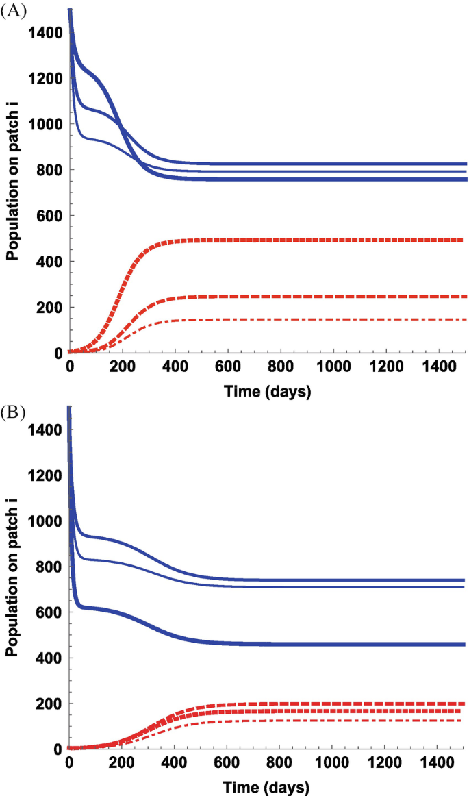

    

    Time plots of the susceptibles (solid) and infectives (dashed) individuals for the resident populations 1 (thicker curve), 2 (intermediate), and 3 (thinner curve). The parameter values used are β = 0.025, κ ₁ = 3, κ ₂ = 2, κ ₃ = 1, g ₁ = 0.01, g ₂ = 0.02, g ₃ = 0.03 in (A) and g ₁ = 0.07, g ₂ = 0.03, g ₃ = 0.04 in (B). All other parameters have the same values as in part (A)

• (c) Consider the same set of parameter values as given in (a) except that the parameters κ ₁ and N ₀₁ for Patch 1 can vary. Numerically plot the solutions for different values of these parameters and describe your observations.

• (d) We can also explore the effect of travel rates g _i on the prevalence. Let β = 0.025 and fix all parameters as in part (b) except g ₁ and κ ₁. Determine a couple of sets of parameter values of g ₁ and κ ₁ that can determine whether or not the infection on Patch 1 can go extinct.

4 Project: A Patch Model with Residence Time

Consider a model consisting of (14.7) and (14.8) with parameters

$$\displaystyle \begin{aligned} N_1 = N_2 = 1{,}000{,}000, \quad \beta_1 =0.3056, \quad \beta_2 = 0.1, \gamma = 1/6.5. \end{aligned}$$

Question 1

Begin with an assumption that mixing is symmetric, p ₁₂ = p ₂₁. Calculate the final epidemic size with several choices of p ₁₁ = p ₂₂.

Question 2

Calculate the effect on epidemic size of assuming no travel to the patch with a higher contact rate by assuming p ₂₂ = 1, p ₂₁ = 0 for several choices of p ₁₂.

Question 3

Calculate the effect on epidemic size of banning all travel, p ₁₂ = p ₂₁ = 0.

References

Anderson, R.M. H. C. Jackson, R. M. May & A. M. Smith (1981) Population dynamics of fox rabies in Europe, Nature, 289: 765–771.
Anderson, R.M. & May, R.M. (1979) Population biology of infectious diseases I, Nature 280: 361–367.
Arino, J. (2009) Diseases in metapopulations, in Modeling and Dynamics of Infectious Diseases, Z. Ma, Y. Zhou, J. Wu (eds.), Series in Contemporary Applied Mathematics, World Scientific Press, Vol. 11; 64–122.
Arino, J., R. Jordan,& P. van den Driessche (2007) Quarantine in a multispecies epidemic model with spatial dynamics, Math. Bisoc. 206: 46–60.
Arino, J. & P. van den Driessche (2003) The basic reproduction number in a multi-city compartmental epidemic model, Lecture Notes in Control and Information Science 294: 135–142.
Arino, J. & P. van den Driessche (2003) A multi-city epidemic model, Mathematical Population Studies 10: 175–93.
Arino, J. & P. van den Driessche (2006) Metapopulation epidemic models, Fields Institute Communications 48: 1–13.
Aronson, D.G. (1977) The asymptotic spread of propagation of a simple epidemic, in Nonlinear Diffusion (W.G. Fitzgibbon & H.F. Walker, eds.), Research Notes in Mathematics 14, Pitman, London.
Bichara, D., Y. Kang, C. Castillo-Chavez, R. Horan & C. Perringa (2015) SIS and SIR epidemic models under virtual dispersal, Bull. Math. Biol. 77: 2004–2034.
Britton, N.F. (2003) Essentials of Mathematical Biology, Springer Verlag, Berlin- Heidelberg.
Capasso, V. (1993) Mathematical Structures of Epidemic Systems, Lect. Notes in Biomath. 83, Springer-Verlag, Berlin-Heidelberg-New York.
Castillo-Chavez, C., D. Bichara, & B. Morin (2016) Perspectives on the role of mobility, behavior, and time scales on the spread of diseases, Proc. Nat. Acad. Sci. 113: 14582–14588.
Diekmann, O. (1978) Run for your life. a note on the asymptotic speed of propagation of an epidemic, J. Diff. Eqns. 33: 58–73.
Diekmann, O. & J.A.P. Heesterbeek (2000) Model building, analysis and interpretation, John Wiley & Sons, New York.
Edelstein-Keshet, L. (2005) Mathematical Models in Biology, Classics in Applied Mathematics, SIAM, Philadelphia.
Espinoza, B., V. Moreno, D. Bichara, & C. Castillo-Chavez (2016) Assessing the Efficiency of Movement Restriction as a Control Strategy of Ebola. In Mathematical and Statistical Modeling for Emerging and Re-emerging Infectious Diseases, pp. 123–145, Springer International Publishing.
Fitzgibbon, W.E., M.E. Parrott, & G.F. Webb (1995) Diffusive epidemic models with spatial and age-dependent heterogeneity, Discrete Contin. Dyn. Syst. 1: 35–57.
Fitzgibbon, W.E., M.E. Parrott, & G.F. Webb (1996) A diffusive age-structured SEIRS epidemic model, Methods Appl. Anal. 3: 358–369.
Grenfell, B.T., & A. Dobson, (eds.)(1995) Ecology of Infectious Diseases in Natural Populations, Cambridge University Press, Cambridge, UK.
Hadeler, K.P. (2003) The role of migration and contact distributions in epidemic spread, in Bioterrorism: Mathematical Modeling Applications in Homeland Security (H. T. Banks and C. Castillo-Chavez eds.), SIAM, Philadelphia, pp. 199–210.
Källén, A. (1984) Thresholds and travelling waves in an epidemic model for rabies, Nonlinear Anal. 8: 651–856.
Källén, A., P. Arcuri & J. D. Murray (1985) A simple model for the spatial spread and control of rabies, J. Theor. Biol. 116: 377–393.
Kot, M. (2001) Elements of Mathematical Ecology, Cambridge University Press.
Lloyd, A. & R.M. May (1996) Spatial heterogeneity in epidemic models. J. Theor. Biol. 179: 1–11.
MacDonald, D.W. (1980) Rabies and Wildlife. A Biologist’s Perspective, Oxford University Press, Oxford.
Mollison, D. (1977) Spatial contact models for ecological and epidemic spread, J. Roy. Stat. Soc. Ser. B 39: 283–326.
Murray, J.D. (2002) Mathematical Biology, Vol. I, Springer-Verlag, Berlin-Heidelberg-New York.
Murray, J.D. (2002) Mathematical Biology, Vol. II, Springer-Verlag, Berlin-Heidelberg-New York.
Murray, J.D., E. A. Stanley & D. L. Brown (1986) On the spatial spread of rabies among foxes, Proc. Roy. Soc. Lond. B229: 111–150.
Ou, C & J. Wu (2006) Spatial spread of rabies revisited: role of age-dependent different rate of foxes and non-local interaction, SIAM J. App. Math. 67: 138–163.
Radcliffe, J. & L. Rass (1986) The asymptotic spread of propagation of the deterministic non-reducible n-type epidemic, J. Math. Biol. 23: 341–359.
Sattenspiel, L. (2003) Infectious diseases in the historical archives: a modeling approach. In: D.A. Herring & A.C. Swedlund, (eds) Human Biologists in the Archives, Cambridge University Press: 234–265.
Sattenspiel, L. & K. Dietz (1995) A structured epidemic model incorporating geographic mobility among regions Math. Biosc. 128: 71–91.
Sun, G.-Q. (2012) Pattern formation of an epidemic model with diffusion, Nonlin. Dyn. 69: 1097–1104.
Thieme, H.R. (1979) Asymptotic estimates of the solutions of nonlinear integral equations and asymptotic speeds for the spread of populations, J. Reine Angew. Math. 306: 94–121.
Turing, A.M. (1952) The chemical basis of morphogenesis, Phil. Trans. Roy. Soc. London B 237: 37–72.
van den Bosch, F., J.A.J. Metz, & O. Diekmann (1990) The velocity of spatial population expansion, J. Math. Biol. 28: 529–565.
van den Driessche, P. (2008) Spatial structure: Patch models, in Mathematical Epidemiology (F. Brauer, P. van den Driessche, J. Wu, eds.), Lecture Notes in Mathematics, Mathematical Biosciences subseries 1945, Springer, pp. 179–189.
van den Driessche P. & J. Watmough (2002) Reproduction numbers and subthreshold endemic equilibria for compartmental models of disease transmission, Math. Biosc. 180: 29–48.
Wang, W.-M,H.-Y. Liu, Y.-L. Cai, & Z.-Q. Li (2011) Turing pattern selection in a reaction-diffusion epidemic model, Chinese Phys. 20: 07472.
Weinberger, H.F. (1981) Some deterministic models for the spread of genetic and other alterations, Biological Growth and Spread (W. Jaeger, H. Rost, P. Tautu, eds.), Lecture Notes in Biomathematics 38, Springer Verlag, Berlin-Heidelberg-New York, pp. 320–333.
Wu, J. (2008) Spatial structure: Partial differential equations models, in Mathematical Epidemiology (F. Brauer, P. van den Driessche, J. Wu, eds.), Lecture Notes in Mathematics, Mathematical Biosciences subseries 1945, Springer, pp. 191–203.
Author information
Authors and Affiliations
Rights and permissions
Copyright information
© 2019 Springer Science+Business Media, LLC, part of Springer Nature
About this chapter
Cite this chapter
Brauer, F., Castillo-Chavez, C., Feng, Z. (2019). Spatial Structure in Disease Transmission Models. In: Mathematical Models in Epidemiology. Texts in Applied Mathematics, vol 69. Springer, New York, NY. https://doi.org/10.1007/978-1-4939-9828-9_14
Download citation
DOI: https://doi.org/10.1007/978-1-4939-9828-9_14
Published:
Publisher Name: Springer, New York, NY
Print ISBN: 978-1-4939-9826-5
Online ISBN: 978-1-4939-9828-9
eBook Packages: Mathematics and StatisticsMathematics and Statistics (R0)