A hierarchical, fuzzy inference approach to data filtration and feature prioritization in the connected manufacturing enterprise

Abstract

In manufacturing, the technology to capture and store large volumes of data developed earlier and faster than corresponding capabilities to analyze, interpret, and apply it. The result for many manufacturers is a collection of unanalyzed data and uncertainty with respect to where to begin. This paper examines big data as both an enabler and a challenge for the connected manufacturing enterprise and presents a framework that sequentially tests and selects independent variables for training applied machine learning models. Unsuitable features are discarded, and each remaining feature receives a crisp numeric output and a linguistic label, both of which are measures of the feature’s suitability. The framework is tested using three datasets employing time series, binary, and continuous input data. Results of filtered models are compared to results obtained by base, unfiltered sets of features using a proposed metric of performance-size ratio. Framework results outperform base feature sets in all tested cases, and the proposed future research will be to implement it in a case study in the electronic assembly manufacture.

Introduction

Rockwell Automation, a global manufacturing and consultation corporation headquartered in Milwaukee, WI, employs a term, The Connected Enterprise (CE), to describe its strategy of corporate shared vision for the future of industrial automation [1]. CE strategies address the problem of disconnect by linking people, equipment, and processes for real-time learning of enterprise status in order to enable informed, adaptive, and proactive decisions [2].

The term “big data” may be loosely defined as information such that the size, structure, or variety strain the capability of traditional software or database tools to capture, store, manage, and analyze it [3, 4]. Not only does big data pose a challenge to software systems and tools, but also the volume of data challenges the ability of human operators, analysts, and leaders to grasp, consume, and understand the critical pieces. Research in fields as diverse as psychology [5], economics [6], and literature [7] have identified limitations in human ability to process, visualize, and synthesize meaning from data. George A. Miller observes that, in a study for which subjects were asked to quickly count the number of dots as they were flashed on a screen, the subjects’ performance on fewer than seven dots so starkly contrasted with performance on more than seven dots that it was given a special name. With fewer than seven dots, subjects “subitized” whereas with above seven dots, subjects “estimated” [5, 8]. Herbert A. Simon observes that information requires attention, and as information increases it necessarily requires the consumer to engage in prioritization, ranking, or filtering to digest it. He also observed that human beings are essentially “serial” creatures, capable of focused attention on only one thing at a time [6]. Finally, the iconic Mortimer J. Adler, in the second edition of How to Read a Book, laments the evolution of a society with vast quantities of knowledge but little depth of understanding [7]. It is interesting to note that these gentlemen wrote their pieces in 1956, 1971, and 1970, respectively. The exploding volume of data captured by modern systems exacerbates this challenge to a degree likely not conceived of at that time [9].

From the definition of big data and the strategies for CE, big data can be seen both as an enabler of the CE as well as an impediment. It is an impediment in that, by definition, it requires innovation and effort to truly harness; it is an enabler in that the successful capture, consumption, and application of big data are precisely the necessary prerequisites to harness the power of the CE to its full potential. The balance between big data as a challenge versus an enabler is illustrated by the “less is more” or “more is less” paradigm. In one sense, the goal is to extrapolate trends from a sample of data, with the smaller the sample the better. Too much data can run the risk of overfitting a model. On the other hand, reducing the data down to a small sample is only a good idea if there is a clear sense of the focus of the analysis. In the quest for latent factors of interest, this strategy may not be advisable. Paradoxically, it may require vast quantities of data in order to train models to identify the narrow sliver of highly valuable information [10]. This is particularly true for highly unbalanced datasets such as defects in a mature manufacturing process. If a small number of key features can be identified to capture the critical information for the decision of interest, then monitoring those key features in the steady state can address the large volume of data [11].

The purpose of this document is to describe and explain a proposed hierarchical data filtration framework for specific application to the connected manufacturing enterprise but that may be generally applied to any big data context. In smart manufacturing, a common observation is that companies collect vast amounts of data but do not effectively analyze or interpret it [12]. This framework addresses a practical aspect of the big-data problem in filtering or discarding data that is not beneficial to the problem at hand; it also speaks to the “human” side of the big-data problem by providing a systematic method to assign a descriptive label to features in a dataset. The value is in providing both analysts and decision-makers additional depth of knowledge regarding the data at their disposal. “Background” section provides background on the concepts underlying the framework. “Methods: proposed framework” section describes the proposed framework. “Results and discussion” section contains application to a dataset, and “Conclusions” section provides concluding remarks and directions for future research. This framework contributes to the big data problem by providing a mechanism to identify value-added features for the problem of interest and, most importantly, quantify the usefulness of those features both numerically and descriptively. At a high level, the framework reduces the number of features to consider by applying a series of filters that first identify features to discard and then highlight quality features to retain for prediction purposes.

Background

The proposed framework integrates four diverse concepts: statistical measures of association, applied metaheuristics, machine learning, and fuzzy inference systems (FIS).

Statistical measures of association

Statistical measures of association attempt to quantify the strength of relationship between sets of data. Four cases are relevant to this paper, indicated in Table 1.

Table 1 Relevant cases for statistical measures of association

The first case is encountered when both the predictor and response variables are categorical. A categorical variable is one that takes on nominal or ordinal values. In this circumstance, the test that immediately comes to mind is Pearson’s Chi Square Test [13]. This hypothesis test computes a test statistic by computing the squared deviation between observed and expected frequencies and then dividing by the expected frequency. This quantity, summed over all possible groups, follows the Chi square distribution and may be tested using conventional hypothesis test procedures.

Pearson’s Chi Square Test, however, is based on the assumption that, within every group, the sample frequencies are normally distributed about the expected population value [14]. Because observed frequencies are nonnegative quantities, small values in any group cast doubt on the validity of the normality assumption. For this reason, Fisher’s Exact Test [15, 16] may be preferable to Pearson’s Chi Square Test when low frequencies are expected in one or more groups. For additional discussion, [17] surveys the development and usage of exact inferential methods for contingency tables.

In the second and third cases, the Kolmogorov–Smirnov Test [18] is used to test whether the distribution of the continuous variable at each level of the categorical variable is the same. In Case 2, the null hypothesis is that the distribution of the response variable is the same when conditioning on each possible level of the predictor. Case 3 uses similar reasoning except that it transposes the target and feature for the purposes of the test. The continuous predictor serves as the target, with its conditional distribution determined at each level of the categorical response.

Finally, in the case of a continuous predictor and a continuous response, Kendall’s rank test [19] is applied.

For a more in-depth treatment of the preceding discussion, as well as application to features extracted from time series data, see [20].

Applied metaheuristics

The question of how to select the best subset of features to apply to a model is an application of the optimal subset problem, which is NP-hard [21] because the number of possible subsets grows exponentially to the size of the domain. For this reason, it is necessary to explore heuristic-based techniques that attempt to achieve good, if not optimal, solutions.

At the most basic level, a local search can be performed. This can be summarized by the following “hill-climbing” process:

• 1. Generate a feasible solution and associated cost function.

• 2. Generate neighborhood solution and associated cost function.

• 3. If cost function improves, store current solution.

• 4. Repeat Step 2 and Step 3 until stopping criteria is achieved.

Most simply, the initial feasible solution and neighborhood solutions may be computed randomly. Alternatively, neighborhood solutions may be computed by slightly perturbing one or more elements of the feasible solution. For example, given an initial feasible solution that includes some number of features out of many possible features, the neighborhood solution might keep all but one feature, drop one feature, and add one feature not previously included.

Clearly, the process described above is crude and, while leading to iteratively-improving feasible solutions, is susceptible to stopping at mediocre solutions found at local optima. Three options to achieve superior results are Tabu Search, Simulated Annealing, and Genetic Algorithm.

Tabu search

Tabu search extends hill-climbing methods by intentionally allowing for the selection of worse solutions when a local optima is obtained, with the incorporation of short-term memory to ensure that previously-visited solutions are not repeated [22]. For detailed background and theory, see [23,24,25,26]. The following procedure, outlined in [24], describes a simple Tabu search. Key to the Tabu search process is the establishment of a set of “off limits” moves that prevent the algorithm from selecting a recently-selected solution.

Notation:

• Let f(x) be the cost function and f*(x) be the best-known objective function value.

• Let x be the current solution.

• Let x* be the best-known solution.

• Let S(x) be the set of all neighborhood solutions about x.

• Let T be the set of prohibited moves, known as the Tabu list.

Procedure:

• 1. As in the hill-climbing process, begin with an initial feasible solution, $x_{0}$, and associated cost function, $f(x_{0} )$. Initially define x* = x = $x_{0}$ and f* = $f(x_{0} )$.

• 2. Generate neighborhood solutions, S(x) and select the best cost function from the set S(x) − T.

• 3. If the cost function improves, define x* = x; if not, no change to x*.

• 4. Update T.

• 5. Repeat Step 2 through Step 4 until stopping criteria is achieved.

Note that there is nothing in the algorithm about local optima. If the best cost function attainable from the neighborhood solutions in Step 2 is worse than the best cost function at x = x*, then the algorithm simply generates a new set of neighborhood solutions and continues until the stopping criteria occurs. Stopping criteria might be some fixed number of iterations, some consecutive number of iterations without an improvement, or some predefined threshold value for the objective function to attain.

Additionally, it should be noted that Tabu search provides significant flexibility to the modeler with respect to how T is defined and how S(x) is defined. The neighborhood structure and tabu list structure can heavily influence the algorithm’s performance. In particular, a neighborhood structure should attempt to move the solution in an intuitively correct direction [22].

Simulated annealing

A second option for achieving superior results to a traditional hill-climbing heuristic is simulated annealing, a term coined for its parallelism with the annealing process in metallurgy. In metallurgy, the process of annealing is a heat treatment procedure by which the alloy is first heated, then held at a certain temperature called the annealing temperature, and then cooled in a controlled manner [27]. The purpose of annealing is to relieve internal stresses, soften, and transform the grain structure of the metal into a more stable state [27].

In simulated annealing, the heuristic allows an inferior solution to be retained according to some probabilistic determination. This helps reduce the risk of converging at a local optimum. As the number of iterations increases, the probability of accepting an inferior solution decreases. The high-level procedure for simulated annealing is as follows [28].

Notation:

• Let f(x) be the cost function and f*(x) be the best-known objective function value.

• Let x be the current solution.

• Let x* be the best-known solution.

• Let S(x) be the set of all neighborhood solutions about x.

• Let k be the index of the current iteration.

• Let T(k) be a temperature parameter.

Note that T(k) is a function of the number of iterations that have taken place. In keeping with the analogy of metallurgical annealing, T begins at a high temperature and gradually decreases over time.

Procedure:

• 1. As previously, begin with an initial feasible solution, $x_{0}$, and associated cost function, $f(x_{0} )$. Initially define x* = x = $x_{0}$ and f* = $f(x_{0} )$. Initialize k = 0.

• 2. Generate neighborhood solutions, $x_{k + 1}$, from $S(x_{k} )$ and the associated $f(x_{k + 1} )$. As previously, the manner of generating neighborhood solutions will likely have a significant effect on the quality of results and the speed of convergence.

• 3. If $f(x_{k + 1} )$ improves from the previous iteration, then x* = $x_{k + 1}$ and f* = $f(x_{k + 1} )$.

• 4. If $f(x_{k + 1} )$ does not improve from the previous iteration:

  • a. Compute p = random (0, 1)

  • b. If $p < exp^{{\left( {\frac{{f\left( {x_{k} } \right) - f\left( {x_{k + 1} } \right)}}{T\left( k \right)}} \right)}}$, then x* = $x_{k + 1}$ and f* = $f(x_{k + 1} )$.

• 5. Increment k = k + 1 and update T accordingly.

• 6. Repeat Step 2 through Step 5 until stopping criteria is achieved.

Note that the above procedure assumes a minimization problem, so that an improvement to f from $x_{k}$ to $x_{k + 1}$ implies that $f(x_{k + 1} ) < f(x_{k} )$. Thus, in Step 4, the quantity $f\left( {x_{k} } \right) - f\left( {x_{k + 1} } \right)$ is negative, which is necessary for the parallelism with metallurgical annealing to hold. Higher values of T(k) result in higher probabilities that an inferior solution will be selected; lower values of T(k) result in lower probabilities.

Simulated annealing has been the subject of extensive research, both theoretical and applied. For additional reading on the theory and application of simulated annealing, see [29, 30]. For textbooks on the subject, see [31, 32].

Genetic algorithms

Genetic algorithms, so named because they employ terminology and techniques that are based on principles of natural selection and genetics, are search methods that evaluate a group of candidate solutions and then evolve subsequent solutions based on the observed attributes in the individual member solutions. The desire is to select and pass on attributes from better solutions and discard the poor solutions and the latent attributes that they carry [33].

Terms and definitions:

• Candidate solutions are referred to as chromosomes and are analogous to the feasible solutions discussed in previous heuristics.

• Elements or sub-components of the chromosomes are referred to as genes, and the values assigned to genes are called alleles.

• Selection refers to the process by which candidate solutions with better fitness values are assigned preference, imposing a survival-of-the-fittest mechanism to the algorithm.

• Recombination refers to the generation of new candidate solutions by merging select elements of two or more solutions identified as having traits conducive to fitness. Solutions designated by the selection process as good are then designated as parent solutions to be combined to produce offspring or child solutions.

• Mutation refers to the process by which the algorithm will randomly modify a child solution by slightly altering one or more of its elements.

Procedure:

• 1. Begin with an initial population of feasible candidate solutions. The starting population is typically obtained randomly, although it is possible to use a more guided method.

• 2. Evaluate each candidate solution using some predefined cost function or measure.

• 3. Select a subset of the population with superior fitness to serve as parent solutions to create the next population of candidate solutions. A number of possible selection strategies exist [34], including but not limited to:

  • a. Select the best n candidate solutions.

  • b. Randomly select n candidate solutions, where the probability that a specific candidate solution is selected is proportional to its fitness.

  • c. Randomly select n groups of k candidate solutions. In each group, the k solutions are compared, and the most fit solution is selected.

• 4. Perform recombination on the selected candidate solutions to generate the next population of candidate solutions. As with selection, there are a number of recombination strategies [35]. Figure 1 illustrates the one-point crossover method.

  Fig. 1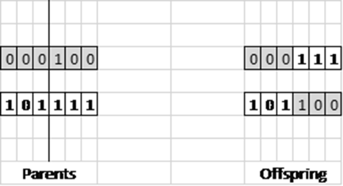

  

  Illustration of one-point crossover recombination

  • a. Select a crossover point. The offspring takes on gene values (alleles) from Parent A (B) for all genes on one side of the crossover point and alleles from Parent B (A) for all genes on the other side of the cross-over point. Two parents produce a total of two offspring.

  • b. Uniform crossover [36]. For each gene, randomly select whether to pass the allele from Parent A or Parent B to the first offspring. The allele from the parent not selected is passed to the second offspring.

• 5. Add variation to the new population through mutation.

• 6. Replace the current population of candidate solutions with the newly-generated population.

• 7. Repeat Step 2 through Step 6 until stopping criteria is achieved.

It could be asked why Step 3(b) and Step 3(c) are options, as they might select inferior candidate solutions to be parents. The reason is simply for the purposes of maintaining genetic variety and maximizing diversity in the gene pool. Additionally, different selection techniques may offer benefits in terms of performance, time to convergence, or computational complexity [34].

Machine learning

Machine learning, as a discipline, intersects several other academic disciplines, most notably computer science, engineering, statistics, and mathematics, with applications in fields as diverse as manufacturing, biology, finance, medicine, and chemistry [37, 38].

It is not the intent of this section to provide a comprehensive overview or tutorial on machine learning, but rather simply to note that the proposed data filtration framework is inextricably linked to the execution of some machine learning algorithm in order to solve some particular problem of interest, initially in the arena of smart manufacturing but not restricted to that discipline.

Specifically relevant to this research are supervised machine learning algorithms for classification or regression. In supervised learning, a set of data exists with known outcomes provided. This data set, called a training set, is then used by the algorithm to develop generalizations or identify patterns in the independent variables to predict the dependent variable. Those generalizations or patterns are then validated using a test set and the model is judged based on appropriate metrics depending on whether the goal is classification (categorical response variable) or regression (continuous response variable).

Fuzzy inference systems

A fuzzy inference system (FIS) is a nonlinear mapping from a given input to a given output established using fuzzy logic and fuzzy set theory [39]. A fuzzy set, in contrast to a crisp set, is a set such that membership is defined along some spectrum or degree [40]. An example of a crisp set might be a component’s status with respect to specification limits. A component is either in tolerance or not in tolerance, and there is no continuum between the two. An example of a fuzzy set might be height status. A person can be considered tall, short, average height, or some other label. Furthermore, a specific individual’s height, such as 5′–6″, might be considered tall in some contexts, short in some contexts, or average in some contexts. A kindergartner who is 5′–6″ tall would be considered tall; a professional basketball player that height would be considered short.

Fuzzy models have been used in applications such as selection, evaluation, decision making, classification, optimization, and prioritization in a diverse array of disciplines [41]. Pioneering work in fuzzy systems was performed by Mamdani, where a Mamdani FIS [42] typically contains four elements: fuzzification, rules, inferencing, and defuzzification [43].

Fuzzification is the process by which a membership function is applied to a crisp input in order to determine the degree of membership in a fuzzy set. For notation purposes, $\mu_{A} \left( x \right)$ denotes the degree of membership in fuzzy set A and is represented by a value between 0 and 1.

Consider a simple example. Suppose that one wishes to use a FIS to label the comfort level of a room. Two important input variables are identified, temperature and humidity, where each can be set at two fuzzy linguistic descriptors: LOW and HIGH. Suppose that the output is the room’s comfort level, which can also be categorized as LOW and HIGH.

The first step would be to define appropriate membership functions for the predictor variables. There are many different options for membership functions [44], including uniform, triangular, trapezoidal, or Gaussian. See Fig. 2 for hypothetical membership functions for this example.

Fig. 2

Membership functions

In Fig. 2, the membership function for temperature is trapezoidal, where a temperature of 40 degrees or less represents full membership in LOW and no membership in HIGH. A temperature of 80 degrees or higher represents full membership in HIGH and no membership in LOW. Temperatures between 40 and 80 vary the degree of membership linearly between LOW and HIGH. A similar interpretation applies to humidity. The response variable, comfort level, is evaluated on a scale from 0 to 100, with a triangular membership function.

Suppose that it is of interest to assign a comfort level to 73° and 65% humidity. Using the above membership functions, fuzzification maps a crisp temperature input of 73° to 0.825 membership in HIGH and 0.175 membership in LOW. A humidity of 65% maps to 0.75 in HIGH and 0.25 in LOW.

Rules are statements in if–then form that relate the input variables to the output variable. For example, a rule might be:

If the temperature is HIGH and the humidity is HIGH, then the comfort level of the room is LOW.

A second rule might be:

If the temperature is LOW and the humidity is LOW, then the comfort level of the room is HIGH.

Inferencing is the application of rules to determine degree of membership in the output. Fuzzy inference systems use logical operators such as AND, OR, or NOT, with different options for how to interpret them. In this example, the operator AND will be defined as the minimum of the two degrees of membership, and OR will be defined as the maximum of the two degrees of membership.

Considering the first rule in our example, the temperature has a degree of membership of 0.825 in HIGH and humidity has a degree of membership of 0.75 in HIGH. This gives the comfort a degree of membership of 0.75 in LOW. Applying the second rule takes the minimum of 0.175 (the temperature’s degree of membership in LOW) and 0.25 (the humidity’s degree of membership in LOW) and assigns it to the degree of membership in HIGH comfort. Figure 3 contains a plot of the membership function of the output variable that accounts for the two rules.

Fig. 3

Membership function for output based on model rules

Defuzzification is a process that takes the fuzzy output and translates it back to a single crisp value. Depending on the context or specific problem of interest, defuzzification may or may not take place. A number of different defuzzification techniques exist [45]. In this example, the centroid technique will be used. The centroid technique computes the center of gravity of the output distribution function and outputs the x-coordinate.

Note that the distributions for each level overlap. Aggregation of rules is typically performed as an OR operation, as illustrated in Fig. 4. Figure 4 also inserts the crisp output based on defuzzification as a vertical line.

Fig. 4

Aggregated output membership with defuzzified result

In our example, the crisp output following defuzzification via the centroid technique is approximately 36.87 out of 100, designated by the vertical line in Fig. 4. This maps to a degree of membership of approximately 0.63 in LOW comfort.

It should be pointed out that the number 36.87 has little meaning in isolation. The contrived example sets an arbitrary scale from 0 to 100 for comfort level. The value would be in comparing the metric derived by 73 degrees and 65 humidity with the metric derived by a different temperature and humidity combination.

Methods: proposed framework

The starting point for the proposed framework, shown in Fig. 5, is a problem of interest and the existence of a population of available data for use both as feature(s) and response(s).

Fig. 5

Proposed framework for data reduction and feature prioritization

Data analysis and preprocessing

The first step is initial data analysis and preprocessing. Of primary interest in this step is the initial identification of a base set of features to apply to the problem of interest. This necessarily involves a high degree of human, subject matter expert involvement. There may arrive a point at which automated processes anticipate future questions and define their own future problems of interest, but, at this point, the initial formulation of the base problem and base set of features is difficult to separate from the human element.

Additional activities during this step may include putting data in a desired format, screening out features based on subject matter expertise, consolidating data from multiple sources, or extracting features of interest from predictor variables. For example, identification of whether any predictor information is time series and extracting time series features would be appropriate for this stage. The algorithm TSFRESH [20], [46] is an excellent tool for extracting features from time series data.

An additional action that may be necessary to perform in this stage is the identification and encoding of data containing categorical features. Different machine learning tools have degrees to which they are compatible with categorical features; some require that each level of the categorical feature be converted to a numeric quantity.

Options exists for how to encode categorical variables, and different techniques have different advantages and disadvantages. A few examples include one-hot encoding, label or ordinal encoding, target mean encoding, and leave-one-out encoding. One-hot encoding replaces N levels with N-1 binary features equal to 1 if the categorical features is at that level and 0 if not. Label or ordinal encoding replaces each level with an integer. Target mean encoding replaces each level with its proportion of occurrence in the target categories. For example, if the categorical variable is gender (M, F) and the response is binary (0, 1), then M and F would be replaced by the proportion of time each gender equals one. Leave-one-out encoding is similar to target mean encoding except that it leaves out the specific record when calculating the proportions.

The output of Step 1: data analysis and preprocessing is a data set that satisfies the preconditions for whichever algorithm or tool is to be applied to the problem of interest. At this point, most frameworks for applied machine learning proceed to identifying the appropriate technique, developing the model, tuning the hyperparameters if necessary, obtaining the model’s results, and then scoring the model using whichever metrics happen to be of interest.

In this case, however, the “problem of interest” is not the only “problem” of “interest”. We are also interested in the data itself and how useful each piece of data is with respect to obtaining the ultimate solution. For this reason, the proposed framework inserts filters that successively eliminate factors from consideration for use in model training.

Filter #1: individual strength of association

The first filter is to apply strength of association hypothesis tests between each feature under consideration and the response variable. This filter individually tests each feature against the response, where the null hypothesis is that the two variables are statistically independent, having no relationship to each other. The hypothesis tests will each produce a p value, which is then compared to the Benjamini–Hochberg threshold [47]; features whose p-values are in tolerance are retained and features whose p-values are not in tolerance are discarded.

The Benjamini–Hochberg test controls the false discovery rate (FDR) at a predefined threshold. The FDR is simply the rate by which random chance allows for the hypothesis test to indicate a significant relationship when there is none. For example, suppose that patients are tested for a disease, where the test has a significance level of 0.05. If 100 patients known to be disease-free are given the test, then by randomness one would expect approximately 5 patients to be erroneously flagged as ill. It is not possible to fully eliminate Type I error, but the Benjamini–Hochberg procedure controls the rate at which it occurs.

$$p_{BH} = \frac{{r_{i} }}{n}*Q$$

(1)

Equation (1) contains the formula for the Benjamini–Hochberg threshold, where $r_{i}$ is the rank of the p-value associated with feature i, n is the number of tests performed, and Q is the required FDR, typically 0.05.

Alternative criteria for determining a threshold p-value do exist, such as the Bonferroni adjustment. The Bonferroni adjustment seeks to control the familywise error rate by proportionately reducing the p-value threshold based on the number of tests performed [48]. If a familywise error rate of 0.05 is desired, and five tests are to be performed, then each test is independently performed with a p-value of 0.01. This is different from Benjamini–Hochberg in that it controls the probability that at least one test will produce a false discovery, in contrast to controlling the rate of false discovery. As a result, the Bonferroni adjustment is more restrictive than Benjamini-Hochberg, allowing fewer features to pass forward. Benjamini–Hochberg is selected for use in this framework because the presence of a second filter makes it less damaging for one or more poor features to be mistakenly lumped in with good features.

Machine learning problem formulation

Up to this point, the specific problem of interest has received only superficial treatment. In Step 1, subject matter expertise was employed to shape the initial set of features, and the data was prepared for use. Step 2 is agnostic to the larger problem of interest or machine learning technique to employ, rather focusing exclusively on any statistical dependence that may exist between an individual feature and the response variable.

At this point, it is necessary to formulate with some degree of specificity the machine learning model to apply to the problem of interest. This includes, at a minimum, designating the machine learning technique and specifying the metrics by which it will be scored. Some techniques, such as random forest, contain hyperparameters that may require tuning.

This step is technically outside the scope of this paper’s primary interest but is included in the framework as a prerequisite to the next filter.

Filter #2: membership in solution groups

After initially testing each feature in isolation against the response variable to determine if there is a statistical dependence between the two, a second filter is applied to the remaining features that examines performance as a member of a collective group. A subset of features is selected, either randomly or according to some intentional process, and used as input for the machine learning algorithm selected in the previous step. The selected features may yield a high-quality solution or a low-quality solution, with quality measured according to those predetermined metrics of interest identified in Step 3. This process is then repeated some number of times until there exists a sufficiently substantial body of high-quality solutions and low-quality solutions to make inferences regarding the specific features that tend to appear in each group.

$$x_{i}^{\left( j \right)} = \frac{{\mathop \sum \nolimits_{k} I_{k}^{\left( j \right)} }}{{K_{i} }}$$

(2)

The proposed convention for computing a numeric value to quantify a feature’s tendency to appear in a group is presented in Eq. (2), where $x_{i}^{\left( j \right)}$ represents the membership of feature $j$ in group i, $K_{i}$ represents the number of subsets in group $i$, and $I_{k}^{\left( j \right)}$ represents an indicator function equal to 1 if feature $j$ is contained in subset $k,$ where $k = 1 \ldots K_{i}$ and 0 if it is not.

There are at least two potentially desirable outcomes from this step. One might simply be to obtain a high-quality solution to the problem of interest. If the set of available features is large, this is a non-trivial undertaking, as the problem to obtain an optimal subset is NP-Hard. In this case, it may be advisable to employ a metaheuristic such as Tabu search, Simulated Annealing, or Genetic Algorithm to allow the solutions to evolve and improve. This approach might best apply when the problem of interest is relatively self-contained and there is not the expectation to extensively generalize its results. If the set of available features is not especially large, it may be economical simply to enumerate every possible combination of features and then select the combination that produces the best result.

A second outcome, more directly aligning with the purpose of this research, is to make a quantified statement of knowledge regarding how useful each remaining feature is with respect to its contribution to the model. For this outcome, achieving a near-optimal subset presents only a partial picture. Suppose, for example, that application of Genetic Algorithm in this step produces an optimal or near-optimal subset of features. A feature’s presence in or absence from that single superior subset does not tell us the same thing about its general usefulness as would the observation that that feature habitually appears in subsets that tend to be good versus subsets that tend to be bad. There will always be the nagging uncertainty as to whether a feature is in the superior subset because it is broadly useful or because its interaction with the other members of the subset produces a uniquely outstanding result.

Feature categorization through fuzzy inference

At this point, the initial set of features has been reduced once by eliminating all features with strong evidence of statistical independence from the response variable. The reduced set of features has subsequently served as the population from which sampling with replacement has created subsets, which have been used as inputs into a machine learning model as appropriate for the problem of interest. As each model is scored by some quality metric, there is a one to one mapping from each feature subset to a scoring metric. Finally, for each feature, a single value has been computed using Eq. (2) for that feature’s association with each group.

Step 5 takes that single value and employs it as a crisp input to a FIS for the purpose of generating a label. This label, applied to each feature, will qualitatively describe the usefulness of the feature. The following set of output labels is proposed for consideration.

• Level 1. This label is for features that produce high quality solutions in single-variable models. Other features receiving this highest level would be those appearing consistently in high-quality solutions but exhibit low or nonexistent membership in low-quality solutions.

• Level 2. This label is for features that exhibit strong membership in high-quality solutions but also exhibit some non-trivial membership in low-quality solutions. This is an indicator that the value contributed by these features is in their interaction with other features in producing a high-quality result.

• Level 3. This label is for features tending not to appear in the best solutions but also tending not to appear in the worst solutions. Rather, these features tend to appear in the “squishy middle”, the subsets of features producing generally unremarkable results.

• Level 4. This label is for features that exhibit strong membership in low-quality solutions but exhibit non-trivial membership in high-quality solutions.

• Level 5: this label is for features that perform poorly regardless of circumstance, exhibiting strong membership in low-quality solutions and low or nonexistent membership in high-quality solutions. These features only contribute to non-poor solutions when they happen to be combined with especially high-performing features.

The strength of this set of labels is in the information it provides. It may be useful to distinguish between features that perform well in isolation and features that only perform well when interacting with other features. Figure 6 contains a plot of the membership function for the more descriptive, 5-level output.

Fig. 6

Membership function, 5-level output

The FIS in this step is constructed according to the following procedure.

• 1. Identification of inputs.

• 2. Definition of input membership functions.

• 3. Definition of rules.

• 4. Fuzzification.

• 5. Activation of rules to create output distribution.

• 6. Defuzzification.

FIS step (1): identification of inputs

It is proposed to employ two fuzzy input variables for each metric of interest. One of the fuzzy input variables will be the feature’s membership in feature subsets producing high quality results and the other fuzzy input variables will be the feature’s membership in feature subsets producing low quality results. Crisp inputs for the FIS are the numerical values obtained by Eq. (2) for each feature’s membership in the high-quality group and the low-quality group.

For example, suppose that the metrics of interest for a classification problem are precision and recall. This FIS would require four fuzzy input variables, as indicated by Table 2.

Table 2 Example fuzzy input variables

FIS step (2): definition of input membership functions

Fuzzy input variables require membership functions, which take the crisp inputs computed in Eq. (2) and convert them into degrees of membership in linguistic labels. For this framework, two linguistic labels are proposed: strong and Weak. One or more middle-ground labels could certainly be considered, but they are omitted because the extra labels add unnecessary complexity to the rule generation step, as will be illustrated below.

As discussed in “Fuzzy inference systems” section, analysts have a host of different membership functions from which to choose. It is proposed to use trapezoidal membership functions, where membership in Low (High) equals one (zero) for $x_{i}^{\left( j \right)} < 0.25$ and equals zero (one) for $x_{i}^{\left( j \right)} > 0.75$. Figure 7 illustrates for a generic, 2-level fuzzy input.

Fig. 7

Membership function, 2-level input

The trapezoidal membership function is selected because it is reasonable to declare a feature as definitively weak or strong when its crisp input is outside of certain parameters.

FIS step (3): definition of rules

The rules definition stage is arguably the most important piece of the FIS because the rules drive the construction of the output distribution. As discussed in “Fuzzy inference systems” section, rules take the IF–THEN form and use logical operators such as AND, OR, and NOT. Table 3 contains the conventions to be employed for the fuzzy logical operators.

Table 3 Fuzzy logical operator conventions

In Table 3, $\mu_{A} \left( x \right)$ refers to the degree of membership of fuzzy input variable A given a crisp input x.

Suggested rules for the five-level output labels are as follows.

• 1. If (Metric = High) is STRONG and (Metric = Low) is WEAK, then Utility is Level 1.

• 2. If (Metric = High) is STRONG and (Metric = Low) is NOT WEAK, then Utility is Level 2.

• 3. If (Metric = High) is WEAK and (Metric = Low) is WEAK, then Utility is Level 3.

• 4. If (Metric = High) is NOT STRONG and (Metric = Low) is NOT WEAK, then Utility is Level 4.

• 5. If (Metric = High) is WEAK and (Metric = Low) is STRONG, then Utility is Level 5.

FIS step (4): fuzzification

The proposed framework imposes no constraints regarding fuzzification. Fuzzification should be implemented as per established FIS conventions as described in “Fuzzy inference systems” section.

FIS step (5): activation of rules

The proposed framework imposes no constraints regarding activation of rules to generate the output distribution. Activation of rules should take place as per established FIS conventions as described in “Fuzzy inference systems” section.

FIS step (6): defuzzification

The proposed framework imposes no constraints regarding defuzzification. Selection of defuzzification technique should take place as per established FIS conventions as described in “Fuzzy inference systems” section.

Results and discussion

Example 1: robot execution failures

Description of data

The proposed framework will be illustrated using a multivariate time series dataset that contains force and torque measurements on a robot after failure detection, obtained via the University of California Machine Learning Archive (https://archive.ics.uci.edu/ml/machine-learning-databases/robotfailure-mld/robotfailure.data.html) [49]. The dataset consists of fifteen instances for each of six different time series variables. There is a variable for force and a variable for torque in each of the x-, y-, and z-directions. The response variable is whether the failure detection turned out to be an actual failure or turned out to be nothing wrong. Out of 88 failures detected, there are 21 false alarms and 67 actual faults.

Data analysis and preprocessing

For this dataset, it is necessary to address two elements. The first element is that the data is divided into two sources, a source for the time series data and a source for the outcome. The second element is that time series data requires an initial step of feature extraction. The Python TSFRESH library is used to extract features from time series data. The algorithm allows for a total of 794 potential features [46] to be extracted from a single time series. For detailed discussion and definitions of potential extracted features, the reader is referred to TSFRESH documentation (https://media.readthedocs.org/pdf/tsfresh/latest/tsfresh.pdf). For this example, TSFRESH extracts a total of 4764 features from the six different time series. The 88 records for each of the new 4764 features are then linked to the corresponding 88 instances of the response variable and then split into training and test sets.

Because the extracted features are all numerical values, it is not necessary to encode any categorical variables.

First filter

Initial filtration through testing each feature individually for statistical dependence with the response variable and then applying the Benjamini–Hochberg threshold reduces the available features from 4764 to 441. This is a reduction of more than 90% in terms of the raw number of features and a reduction of approximately 80% in terms of the size of the data. As for feature extraction, the Python TSFRESH library has user-friendly functionality to quickly cycle through the hypothesis tests in this step [46].

Machine learning problem formulation

At this point, the dataset containing the 88 records for the reduced set of features could be used to train a classification model. For the proposed framework, formulation of the machine learning problem is a necessary precondition to applying the second filter.

Our example of attempting to predict robot execution failures is a classification problem with a binary response variable. Somewhat arbitrarily, support vector machines (SVM) is selected as the technique, with the software engine being Python’s “sklearn” [50] library and the “svm” package. Because the proposed framework is concerned with features’ relative value compared to each other, there was no attempt made in this example of tune or optimize hyperparameters; rather, default settings were used. In sklearn, the kernel function defaults to radial bias function (RBF) and a kernel coefficient of 1/(# features) [51].

The 88 records were divided 80% into the training set and 20% into the test set. Due to rounding, this translates to 70 records in the training set and 18 records in the test set.

Second filter

The number of features remaining after the first filter in Step 2 is 441, a number that is prohibitively large if the desire is to obtain the optimal subset of features. The number of subsets that could be generated by a set of this size is approximately 5 × 10¹³³. If it were possible to check one million subsets every second, it would still take approximately 1.8 × 10¹¹⁹ years to iterate through every possible subset.

A total of N = 1000 subsets of size K = 5 each were randomly generated and used to train the machine learning algorithm described in “Summary of results” section. Applying the trained model to a test set and scoring the results in each of the 1000 subsets using Cohen’s Kappa, subsets were either designated as “High Quality”, “Low Quality” or discarded. High Quality solutions were defined as those with a Cohen’s Kappa statistic greater than 0.85. Low Quality solutions were defined as those with a Cohen’s Kappa statistic less than 0.15. Out of 1000 subsets, 58 were placed in the High Quality group and 446 were placed in the Low Quality group. The remaining 496 subsets scored between 0.15 and 0.85 and were not placed in either group. Crisp inputs for each feature in each group were obtained using Eq. (2).

Due to the high number of subsets in the two groups, one adjustment was necessary to Eq. (2). The large $K_{i}$ for each group resulted in very small values for the $x_{i}^{\left( j \right)}$. To reward the better-performing features, the value obtained in Eq. (2) was normalized by dividing each one by the highest $x_{i}^{\left( j \right)}$ attained, as indicated by Eq. (3).

$${x^{\prime}}_{i}^{\left( j \right)} = \frac{{x_{i}^{\left( j \right)} }}{{{ \hbox{max} }\left( {x_{i}^{\left( j \right)} } \right)}}$$

(3)

This adjustment better allows the crisp inputs to map to intuitive fuzzy labels in the FIS stage of the framework.

Fuzzy inference system

The FIS for this problem contains two input variables. High Quality group membership and Low Quality group membership. For each variable, a 2-level membership function was employed as indicated by Fig. 8. The crisp input for each input variable is calculated using Eq. (3).

Fig. 8

FIS results for Robot Failure example

The output variable is denoted as Value and uses five levels as described in “Methods: proposed framework” section. Figure 8 contains an extract from a Microsoft Excel spreadsheet of the FIS crisp inputs, degrees of membership determined by fuzzification, rule results, crisp output calculated in the defuzzification step using the centroid method, and finally a degree of membership for the crisp output based on the aggregated output distribution generated by the FIS.

Consider the output for Row 2, corresponding to Feature 0. Out of the 58 subsets in the High Group, exactly two contained Feature 0. The highest number of subsets in which any of the 441 features appears is five, giving a normalized crisp input of 0.4. Applying the trapezoidal membership function for the High Group fuzzy input, degrees of membership of 0.7 in WEAK and 0.3 in STRONG are obtained and found in cells C2 and D2 respectively.

Similar reasoning and calculations give the values in cells E2, F2, and G2. For cell E2, Feature 0 is present in 4 out of 446 Low Group subsets; this value is normalized by dividing by the maximum number for any feature, which happens to be 15 in this case.

Columns H2, I2, J2, K2, and L2 give the outputs for each rule applied to Feature 0. To illustrate, consider cell H2 for Rule 1. Rule 1 takes the minimum of the feature’s degree of membership in High_STRONG (0.3) and Low_WEAK (0.967) and applies it to L1. This applies a value of 0.3 to the output distribution for the L1 label. Similar application of rules two through five give the remaining values.

Column M provides the crisp, defuzzified output, calculated using the centroid technique. The centroid technique computes the center of mass of the output distribution and returns the coordinate for the horizontal axis. For this model, defuzzification was performed using Python’s skfuzzy [52] package, a fuzzy toolkit for the scikit-learn [50] library.

Finally, Column N gives the degree of membership of the crisp output in the output distribution. Let $DOM_{o}$ be the output degree of membership. If this value is less than one, then the interpretation is to apply it to whichever label is indicated by the output distribution. In this problem, the output membership function is defined such that not more than two labels will overlap. It is possible to interpret the quantity $1 - DOM_{o}$ as be the degree of membership in the other label. However, caution should be applied when doing so because this could result in conflict with one or more rule results. Figure 9 illustrates for Feature 0.

Fig. 9

Output distribution and crisp output for Feature 0 in Robot Failure example

The black vertical line represents the crisp output, and its point of intersection with the L3 label boundary corresponds to a value of approximately 0.5237 on the vertical axis, as indicated in Cell N2 of Fig. 8.

Note that the highlighted portions of the output distribution correspond to the rule outputs, with overlaps defaulting to the higher value. In this case, it is not advisable to interpret Feature 0 as having a degree of membership of 0.5237 in L3 and 0.4763 in L2 because that would conflict with Rule 2, which applies a value of only 0.033 to the output distribution for L2. Stated differently, because Rule 2 prohibits Feature 0 from having a degree of membership in L2 that exceeds 0.033, one cannot infer a degree of membership of 0.4763 from the defuzzified output.

Results

Out of 441 features, the model categorizes 15 at Level 1, or features of the highest value. The model categorizes 76 features at either Level 5 or Level 4, the two lowest-value labels. Table 4 summarizes the results.

Table 4 Feature classification summary for robot failure example

Discussion

The first immediate observation from this example is that none of the 441 features were classified as L5 and only two are classified as L2. This may be a sound result or it may be indicative of an anomaly or suboptimal element in the FIS.

It is possible that sampling only 1000 subsets was not a sufficient number to ensure that the features are appropriately distributed across the output labels. This hypothesis may be supported by the large number of features in the “squishy middle”, showing neither strong membership in the High Quality group nor weak membership in the Low Quality group. To test this, the model was run again, this time taking 200,000 random subsets instead of the initial 1000. Results are displayed in Table 5.

Table 5 FIS results (200,000 subsets)

The results in Table 5 are not substantially different from those obtained in Table 3, the most noticeable difference being features shifted from Level 3 to Level 4.

A second possible explanation is that a 2-level fuzzy input variable is not sufficiently descriptive to give adequate treatment to one or more rules. For example, Rule 2 attempts to capture the situation by which a feature shows strong presence in high quality solutions and a not-weak presence in low quality solutions. However, with only two labels for the fuzzy input variables, a not-weak presence in low quality solutions is not distinguishable from a strong presence in low quality solutions.

Figure 10 contains an alternative membership function for the two fuzzy input variables, this time containing three levels: STRONG, MODERATE, and WEAK.

Fig. 10

Membership function for 3-level input membership function

Table 6 contains model results for the modified FIS, generated using 1000 subsets.

Table 6 Modified FIS results, using 3-level input membership function

This small change to the FIS results in a marked improvement in the results from a plausibility perspective. It is entirely reasonable to expect that the smallest number of features will reside at the extremes; in this case, two features are designated Level 1 and no features are designated Level 5. It is also reasonable to expect that most features would not be especially useful. Considering the Pareto principle [53,54,55]—if most variation can truly be explained by a relatively small number of variables, then it is natural to expect increasing numbers of features to be classified in the lower value categories.

A second point of discussion is sensitivity analysis. It has already been demonstrated that increasing the number of randomly generated subsets from 1000 to 200,000 does not substantially change the numbers of features assigned to each level of value. However, upon closer examination, it is revealed that the two scenarios do not necessary flag the same features in the same way. Put in different words, it is not clear the extent to which model replications consistently assign the same labels to the same features. Table 7 lists the top 15 features for each scenario, rank ordered by their defuzzified crisp outputs.

Table 7 Comparison of best feature categorization, 2-level input membership functions

Table 7 shows that there is almost no overlap between the top fifteen features in each scenario, with only one feature, Feature 22, appearing in both lists. One possible explanation might, again, be the number of subsets in the two samples. Perhaps, for 441 features to consider, 1000 subsets is too few to generate consistent results.

To test this hypothesis, the model was run n = 10 times with k = 10,000 subsets each run. Figure 11 contains an extract of Microsoft Excel output with the top performing features in each run and the aggregated results.

Fig. 11

Highest-ranked FIS output for 10 runs, 10,000 subsets per run

Columns L and M give aggregated counts for how many times each feature appears in the Top 15 performing features, summed over the ten runs. Out of 441 features, 427 appear fewer than three times, and only five features appear seven or more times. Those five features, which consistently score highly in the FIS, are candidates to retain.

A third point of discussion follows directly from the sensitivity analysis. The example in this paper that began in “Example 1: robot execution failures” section started with 4764 features, reduced to 441 following Filter #1, and has been potentially reduced to five at the culmination of the proposed framework. However, this reduction is only acceptable if the remaining features produce acceptable solutions to the problem of interest.

Two questions are necessary to answer. The first is if solutions produced by the final, reduced set of features will generate comparable results to the solutions produced by the full set of features. The second is if those solutions are acceptable to be used for their intended decision-making purposes.

The full model, using all 441 features, performs extremely poorly in this case. Likely due to overfitting, a model trained on 80% of the dataset and tested on 20% of the dataset makes the same prediction for all records in the test set. Table 8 contains the confusion matrix.

Table 8 Confusion matrix using all 441 features

In contrast, Table 9 contains the confusion matrix for a model generated using the top five features from Fig. 12. The refined model perfectly classifies the 18-record test set.

Table 9 Confusion matrix using best-rated features from FIS

Fig. 12

Consolidated FIS results

It should be clarified that, for this example, support vector machines was selected as the machine learning algorithm to use not because it is ideal or performs especially well, but rather to illustrate the contrast between model performance with the full set of features versus the reduced set of features. Had an alternative technique been chosen, such as classification trees or random forest, the contrast may have been less pronounced.

A final point of discussion will be the introduction of a metric to quantify the relationship between relative performance and relative size of the different models generated by the various stages and filters in the framework.

$$PSR = \frac{Model\, relative\,\,performance}{Model \,relative\, size} = \frac{{{\raise0.7ex\hbox{${M_{i} }$} \!\mathord{\left/ {\vphantom {{M_{i} } {M_{0} }}}\right.\kern-0pt} \!\lower0.7ex\hbox{${M_{0} }$}}}}{{{\raise0.7ex\hbox{${S_{i} }$} \!\mathord{\left/ {\vphantom {{S_{i} } {S_{0} }}}\right.\kern-0pt} \!\lower0.7ex\hbox{${S_{0} }$}}}}$$

(4)

This metric, denoted as PSR, is the performance-size ratio for a given model at some stage in the framework. In Eq. (4), $M_{i}$ represents the performance of the model after Step i in the proposed framework, $M_{0}$ represents the performance of the base model with no feature reduction, $S_{i}$ represents the size of the model after Step i, and $S_{0}$ represents the size of the base model with no reduction.

Example 2: single proton emission computed tomography (SPECT) images

Description of data

A second example illustrates the proposed framework on a dataset describing the diagnosing of cardiac SPECT images, obtained from the University of California Machine Learning Archive (http://archive.ics.uci.edu/ml/machine-learning-databases/spect/SPECT.names) [49]. The dataset consists of 267 SPECT image sets, each image set corresponding to a single patient. The response variable is a binary classification of normal (0) or abnormal (1). A total of 22 binary feature patterns serve as the initial set of predictor variables.

Of the 267 SPECT image sets, 55 are classified as normal and 212 are classified as abnormal. The breakdown of data by classification after splitting the data into training and test sets is provided in Table 10.

Table 10 Composition of SPECT data for example 2

Problem formulation

For Step 1: data analysis and preprocessing, this dataset requires relatively little action. There is no time series component, requiring no feature extraction step. Likewise, there are no categorical features, requiring no encoding of categorical variables.

For Step 3, classification trees are selected as the machine learning technique, with default Python sklearn.tree.DecisionTreeClassifier() settings applied.

For Step 4, classification accuracy was employed as the metric for determining whether a subset falls into the High Quality group or the Low Quality group. Classification accuracy is defined as the number of correctly predicted test set records divided by the total number of test set records.

For 1000 subsets of N = 5 features per subset, the range of classification accuracies was approximately 0.62–0.87. Given these values, a threshold of 0.75 was set, where subsets whose solution’s classification accuracy exceed 0.75 were placed in the High Quality group and those not were placed in the Low Quality group.

For Step 5, ten runs of N = 1000 subsets with k = 5 features per subset were run, and the top five scoring features were recorded. This is largely the same as in “Example 1: robot execution failures” section, with the exception that the top 15 features in that example were truncated due to the large number of features remaining. FIS parameters such as membership functions and rules were unchanged.

Figure 12 contains a screen shot of a Microsoft Excel spreadsheet summarizing the results.

Summary of results

Filter #1 reduced the initial set of 22 features to 15. After applying Filter #2 and FIS classification, six features stood out predominantly as consistently being scored by the FIS as among the top five features in a given run.

Table 11 summarizes the model performance for each of three cases: the original model with no feature reduction, the reduced feature set after Filter #1, and the final reduced feature set following the FIS.

Table 11 Summary of model performance

Using the original, unfiltered model as a baseline, Table 11 shows that the model, after applying Filter #1, displays a slight degradation in performance regarding classification accuracy but ends up with a higher PSR due to the reduced size required in the model. The final model produces a superior classification accuracy with 0.2727 the input size, resulting in a PSR of approximately 3.8416.

Example 3: single proton emission computed tomography image features (SPECTF)

Description of data

A third example uses the SPECTF dataset (http://archive.ics.uci.edu/ml/machine-learning-databases/spect/SPECTF.names), obtained using the same 267 SPECT images from “Example 2: single proton emission computed tomography (SPECT) images” section. The difference is that, in this case, 44 continuous features instead of 22 binary features are extracted from each image. No change to the response variable.

Problem formulation

For Step 1: data analysis and preprocessing, this dataset requires relatively little action. There is no time series component, requiring no feature extraction step. Likewise, there are no categorical features, requiring no encoding of categorical variables.

For Step 3, random forest is selected as the machine learning technique, with default Python sklearn.ensemble.RandomForestClassifier() settings applied. As with the previous two examples, the specific machine learning technique is not central to the model. Any algorithm for classification could have been chosen.

For Step 4, classification accuracy was again employed as the metric for determining whether a subset falls into the High Quality group or the Low Quality group.

For 1000 subsets of N = 5 features per subset, the range of classification accuracies was approximately 0.62–0.87. Given these values, a threshold of 0.75 was set, where subsets whose solution’s classification accuracy exceeds 0.75 are placed in the High Quality group and those not are placed in the Low Quality group.

For Step 5, ten runs of N = 1000 subsets with k = 5 features per subset were run, and the top five scoring features were recorded. FIS parameters such as membership functions and rules are unchanged from the previous two examples.

Summary of results

Filter #1 reduced the initial set of 44 features to 18. After applying Filter #2 and FIS classification, five features stood out predominantly as consistently being scored by the FIS as among the top five features in a run.

Table 12 summarizes the model performance for each of three cases: the original model with no feature reduction, the reduced feature set after Filter #1, and the final reduced feature set following the FIS.

Table 12 SPECTF example results

Using the original, unfiltered model as a baseline, Table 12 illustrates that the model after applying Filter #1 displays a slight degradation in performance. This is similar to the results observed in the SPECT example in “Example 2: single proton emission computed tomography (SPECT) images” section. Examining the confusion matrices produced by the original model and the model after applying Filter #1, the difference amounts to four additional misclassified records. This near-attaining of the performance of the original model happens at an almost 60% reduction in the size of the feature set.

Two “final” models are defined and scored. The first keeps the best features, as identified by the FIS. This final model produces a slightly improved classification accuracy of 0.8703 with 0.1364 the input size, resulting in a PSR equal to approximately 7.8308. A second way to determine the final feature set to retain is to drop the worst-performing features as ranked by the FIS. This model produces a slightly superior classification accuracy of 0.8333. This is an improvement over both the original feature set and equal to the performance of the set of best-performing FIS features. The PSR for the two “final” models favors the model obtained by keeping the best-performing features by virtue of the smaller size of its feature set. This result also demonstrates, for this dataset, that there is a middle-ground subset of features that are not classified as “worst” by the FIS but offer no added value to the overall scoring of the solution.

Conclusions

This paper’s contribution is in the integration of diverse techniques and disciplines of statistical independence tests, applied machine learning, and fuzzy inference systems in such a way that, as yet, has not been undertaken previously.

The proposed framework presented in this paper attempts to rank and classify potential predictor variables according to their value for use in training machine learning models for some problem of interest. This contributes to the general methodology of machine learning design and adds a dimension of knowledge related to the dataset for analysts and decisionmakers to apply not only to the current problem but also in subsequent analyses or related projects.

Up to this point, the proposed framework has only been tested on publicly available machine learning datasets. The next step is to test the framework on a practical, applied case study in the CE.

Future research will explore the proposed framework in the context of electronic assembly manufacture, specifically the pick-and-place (P&P) operation in the assembly process of printed circuit boards (PCBs). The P&P operation uses surface mount technology (SMT) to mount parts, especially the smaller low-voltage, low-power components onto a PCB. Typically, the P&P process involves the stages presented in Fig. 13. Though the process may vary from company to company and by component size, generally, the boards are loaded, screen-printed, and inspected for solder defects. Next, chips and components are surface mounted onto the PCB at the P&P machines, hereby named Mach 1 and Mach 2. Generally, components vary size-wise from less than an eighth of a millimeter to several centimeters in diameter (length). They are mounted onto the PCBs through automated control systems. Once mounted, the PCBs are conveyed to the reflow oven where, at high temperatures, the solder is melted to bind the components onto the PBCs. Finally, the PCBs are optically inspected and sent further downstream either for assembly or warehousing.

Fig. 13

PCB P&P process

Continued miniaturization and increased density of components on a PCB have increased the potential for quality defects, thus the criticality of P&P process in the PCB assembly process.

Additionally, future research can explore and quantify the sensitivity of the proposed framework to the machine learning problem formulation in Step 3, the hyperparameters in Step 4: filter #2, and the FIS parameters in Step 5 in order to identify rules of thumb for hyperparameter tuning. In particular, there is tremendous variety in how Filter #2 could be applied. This paper randomly generated feasible solutions of a fixed size; using a metaheuristic such as Tabu Search, Genetic Algorithm, or Simulated Annealing could provide advantages to the feature selection that might influence how the FIS in Step 5 is constructed.

Finally, the proposed framework is entirely in the realm of supervised learning. Additional research can explore extending the framework to problems of interest in the realms of unsupervised or reinforcement machine learning.

References

Rockwell Automation. The connected enterprise ebook: bringing people, processes, and technology together. Milwaukee: Rockwell Automation; 2015.
Otieno W, Cook M, Campbell-Kyureghyan N. Novel approach to bridge the gaps of industrial and manufacturing engineering education: A case study of the connected enterprise concepts. In: Proc. Front. Educ. Conf. FIE. 2017. p. 1–5.
Qin SJ. Process data analytics in the era of big data. AIChE J. 2014;60(9):3092–100.
McKinsey & Company. Big data: The next frontier for innovation, competition, and productivity. New York: McKinsey Glob. Inst.; 2011.
Miller GA. The magical number seven, plus or minus two: some limits on our capacity for processing information. Psychol Rev. 1956;63(2):81–97.
Simon HA. Designing organizations for an information-rich world. Comput Commun Public Interest. 1971;72:37.
Adler MJ, Van Doren C. How to read a book: the classic guide to intelligent reading. New York: Simon and Schuster; 1972.
Kaufman EL, Lord MW, Reese TW, Volkmann J. The discrimination of visual number. Am J Psychol. 1949;62(4):498–525.
Mourtzis D, Vlachou E, Milas N. Industrial big data as a result of IoT adoption in manufacturing. Procedia CIRP. 2016;55:290–5.
D. Bollier and C. M. Firestone, The Promise and Peril of Big Data. 2010.
He QP, Wang J. Statistical process monitoring as a big data analytics tool for smart manufacturing. J Process Control. 2017;67:35–43.
Kusiak A. Smart manufacturing must embrace big data. Nature. 2017;544(7648):23–5.
Pearson K. X. On the criterion that a given system of deviations from the probable in the case of a correlated system of variables is such that it can be reasonably supposed to have arisen from random sampling. Philos Mag Ser. 1900;50(302):157–75.
Vinet L, Zhedanov A.Chi Square Test, in encyclopedia of research design, vol. 44, no. 8, 2455 Teller Road, Thousand Oaks California 91320 United States: SAGE Publications, Inc., 2011, p. 085201.
Fisher RA. On the interpretation of X2 from contingency tables, and the calculation of P. J R Stat Soc. 1922;85(1):87–94.
Fisher RA. Statistical methods for research workers, fourteenth. Edinburgh: Oliver & Boyd; 1970.
Agresti A. A survey of exact inference for contingency tables. Stat Sci. 1992;7(1):131–53.
Massey FJJ. The Kolmogorov–Smirnov test for goodness of fit. J Am Stat Assoc. 1951;46(253):68–78.
Kendall MG. A new measure of rank correlation. Biometrika. 1938;30(1):81–93.
Christ M, Kempa-Liehr AW, Feindt M. Distributed and parallel time series feature extraction for industrial big data applications. 2016.
Binshtok M, Brafman RI, Shimony SE, Martin A, Boutillier C. Computing optimal subsets. In: Proc. 22nd Natl. Conf. Artif. Intell. 2007. p. 1231–6.
Gendreau M, Potvin J-Y. Tabu Search. In: Burke EK, Kendall G, editors. Search methodologies: introductory tutorials in optimization and decision support techniques. 2nd ed. New York: Springer; 2014. p. 243–64.
Glover F. Future paths for integer programming and links to artificial intelligence. Comput Oper Res. 1986;13(5):533–49.
Glover F. Tabu search—part I. ORSA J Comput. 1989;1(3):190–206.
Glover F. Tabu search—part II. ORSA J Comput. 1990;2(1):4–32.
Glover F, Laguna M, Marti R. Principles of tabu search. Approx Algorithms Metaheuristics. 2007;23:1–12.
Kopeliovich D. Basic principles of heat treatment. SubsTech: Substances & Technologies, 2012. http://www.substech.com/dokuwiki/doku.php?id=basic_principles_of_heat_treatment. Accessed 24 Jul 2018.
Aarts E, Korst J, Michiels W. Simulated Annealing. In: Burke EK, Kendall G, editors. Search methodologies: introductory tutorials in optimization and decision support techniques. 2nd ed. New York: Springer; 2014. p. 265–86.
Kirkpatrick S, Gelatt CD, Vecchi MP. Optimization by simulated annealing. Science (80−). 1983;220(4598):671–80.
Henderson D, Jacobson SH, Johnson AW. The Theory and practice of simulated annealing. In: Glover F, Kochenberger GA, editors. Handbook of metaheuristics. Boston: Kluwer Academic Publishers; 2003. p. 287–319.
Aarts E, Korst J. Simulated annealing and boltzmann machines: a stochastic approach to combinatorial optimization and neural computing. New York: Wiley; 1989.
van Laarhoven PJM, Aarts EHL. Simulated annealing: theory and applications. Boston: Kluwer Academic Publishers; 1987.
Sastry K, Goldberg DE, Kendall G. Genetic algorithms, in Search methodologies: introductory tutorials in optimization and decision support techniques. New York: Springer; 2014. p. 93–117.
Goldberg DE, Deb K. A comparative analysis of selection schemes used in genetic algorithms. Found Genet Algorithms. 1991;1:69–93.
Golberg DE. Genetic algorithms in search optimization & machine learning. Reading: Addison-Wesley; 1989.
Syswerda G. Uniform crossover in genetic algorithms. In: Proceedings of the third international conference on genetic algorithms: George Mason University, San Mateo, CA. New York: M. Kaufmann Publishers; 1989. p. 2–9.
Marsland S. Machine learning: an algorithmic perspective. 2nd ed. Boca Raton: CRC Press; 2015.
Carbonell JG, Michalski RS, Mitchell TM. An overview of machine learning. In: Michalski RS, Carbonell JG, Mitchell TM, editors. Machine learning: an artificial intelligence approach. Palo Alto: Tioga Publishing Company; 1983. p. 3–23.
Mendel JM. Fuzzy logic systems for engineering: a tutorial. Proc IEEE. 1995;83(3):345–77.
Zadeh LA. Fuzzy sets. Inf Control. 1965;8(3):338–53.
Omwando TA, Otieno WA, Farahani S, Ross AD. A Bi-level fuzzy analytical decision support tool for assessing product remanufacturability. J Clean Prod. 2018;174:1534–49.
Mamdani EH. Application of fuzzy algorithms for control of simple dynamic plant. Proc Inst Electr Eng. 1974;121(12):1585.
Yildiz YC. A short fuzzy logic tutorial. 2010. p. 1–6.
Hong TP, Lee CY. Induction of fuzzy rules and membership functions from training examples. Fuzzy Sets Syst. 1996;84(1):33–47.
Saletic D, Velasevic D, Mastorakis N. Analysis of basic defuzzification techniques. In: 6th WSES Int. Multiconference Circuits, Syst. Telecomunications Comput, 2002. p. 7–14.
Christ M, Braun N, Neuffer J, Kempa-Liehr AW. Time series feature extraction on basis of scalable hypothesis tests (tsfresh—A Python package). Neurocomputing. 2018;307:72–7.
Benjamini Y, Yekutieli D. The control of the false discovery rate in multiple testing under dependency. Ann Stat. 2001;29(4):1165–88.
Howell DC. Multiple comparisons among treatment means, in statistical methods for psychology. 8th ed. Boston: Cengage Learning; 2012. p. 384–7.
Dheeru D, Karra Taniskidou E. UCI Machine Learning Repository. University of California, Irvine, School of Information and Computer Sciences, 2017.
Pedregosa F, Varoquaux G, Gramfort A, Michel V, Thirion B, Grisel O, Blondel M, Prettenhofer P, Weiss R, Dubourg V, Vanderplas J, Passos A, Cournapeau D, Brucher M, Perrot M, Duchesnay É. Scikit-learn: machine learning in python. J Mach Learn Res. 2012;12:2825–30.
“sklearn.svm.SVC,” Scikit-learn version 0.19.2 Online documentation. http://scikit-learn.org/stable/modules/generated/sklearn.svm.SVC.html#sklearn.svm.SVC. Accessed 21 Aug 2018.
Warner J, Sexauer J, Twmeggs AM, Unnikrishnan A, Castelão G, Batista F, Badger TG, Mishra H. JDWarner/scikit-fuzzy: Scikit-Fuzzy 0.3.1, 2017.
Flaum SA. Pareto’s Principle. Pharmaceutical executive. vol. 27, no. 2, Duluth, 2007. p. 54–6.
Harvey HB, Sotardi ST. The pareto principle. J Am Coll Radiol. 2018;15(6):931.
Gupta P. The pareto principle. Printed circuit fabrication, vol. 24, no. 1, San Francisco. 2001, p. 62–3.
Authors’ contributions
FM provided subject matter expert review and content for “Introduction” section and “Conclusion—Summary and future research” section, for details regarding the Connected Enterprise and applied case study in electronic assembly manufacture. WO provided subject matter expert review and content regarding the Connected Enterprise in “Introduction” and proposed framework in “Methods” section: PL provided subject matter expert review and content for “Background” section, developed the proposed framework in “Methods” section, and conducted the experiment and follow-on analyses in “Results and discussion” section. Additionally, PL performed authorship functions of assembling the initial draft, editing, and serving as corresponding author. All authors listed have materially participated in the research and/or preparation and have approved of the final submission. All authors read and approved the final manuscript.
Acknowledgements
Not applicable.
Competing interests
The authors declare that they have no competing interests.
Availability of data and materials
The datasets generated in this study are available from the UCI Machine Learning Repository (https://archive.ics.uci.edu/ml/index.php).
Example #1 data: https://archive.ics.uci.edu/ml/machine-learning-databases/robotfailure-mld/robotfailure.data.html.
Example #2 data: https://archive.ics.uci.edu/ml/machine-learning-databases/spect/SPECT.names.
Example #3 data: https://archive.ics.uci.edu/ml/machine-learning-databases/spect/SPECTF.names.
Funding
The authors affirm that there are no sources of funding for the research to be declared.
Publisher’s Note
Springer Nature remains neutral with regard to jurisdictional claims in published maps and institutional affiliations.
Author information
Authors and Affiliations
Corresponding author
Rights and permissions
Open Access This article is distributed under the terms of the Creative Commons Attribution 4.0 International License (http://creativecommons.org/licenses/by/4.0/), which permits unrestricted use, distribution, and reproduction in any medium, provided you give appropriate credit to the original author(s) and the source, provide a link to the Creative Commons license, and indicate if changes were made.
About this article
Cite this article
LaCasse, P.M., Otieno, W. & Maturana, F.P. A hierarchical, fuzzy inference approach to data filtration and feature prioritization in the connected manufacturing enterprise. J Big Data 5, 45 (2018). https://doi.org/10.1186/s40537-018-0155-2
Received:
Accepted:
Published:
DOI: https://doi.org/10.1186/s40537-018-0155-2