
Abstract
This paper reports the results of a seismic performance study of a precast shear wall with a new horizontal connection. The new connection is the rabbet-unbonded horizontal connection, which is composed of rabbets and unbonded rebar segments. The rabbets are used to improve the shear capacity and prevent slippage of the connection, and the unbonded rebar segments are used to improve the ductility and energy dissipation. Three specimens were tested with different parameters under cyclic quasi-static loading. The test results showed that the specimen with a larger unbonded level had a richer hysteresis curve, larger ductility, larger energy dissipation, and slightly smaller bearing capacity. Moreover, in relation to the stiffness degradation, in the initial stage, the specimen with a larger unbonded level had a smaller stiffness, whereas in the last stage, the stiffnesses were similar regardless of the unbonded level. A parameter analysis using a finite element model proved that the ductility and energy dissipation of a shear wall with the rabbet-unbonded horizontal connection increased with the unbonded length and level. In addition, when the axial compression ratio increased, the bearing capacity increased, but the load–displacement curves decreased more rapidly. It was concluded that the unbonded length and unbonded level could effectively improve the ductility and energy dissipation of a shear wall. However, they should not be too large under high pressure, and the design suggestions for the new connection need further research considering other factors.
1 Introduction
Compared to the traditional construction method, building prefabrication has the characteristics of high production efficiency, high construction quality, resource savings, reduced energy consumption, and low noise pollution, and is widely used in China and other countries. Among the many precast structural forms, the precast shear wall structure is the first choice for multi-storey and high-rise buildings because of its large lateral stiffness and bearing capacity (Perez and Mauricio 2018).
For a precast shear wall structure, the horizontal connection is the key to ensure structural integrity and seismic performance, and to date, the most commonly used connections include the unbonded post-tensioned (UPT) connection, bolted connection, and grouting connection (Sorensen et al. 2017; Elsayed et al. 2018).
For the UPT connection, a series of tests and analytical studies have been performed on unbonded post-tensioned precast concrete wall structures (Zhu and Guo 2018; Buddika and Wijeyewickrema 2018; Lu et al. 2018; Gu et al. 2019; Yang and Lu 2018). A UPT structure has the advantages of a good self-recovery ability, and the potential ability to decrease the residual drifts and reduce the structural damage. However, it has the disadvantage of poor energy dissipation. In view of this, many scholars have investigated improvement measures to improve its energy dissipation capacity, such as adding energy-consuming connectors (Twigden and Henry 2019), friction connectors (Guo et al. 2018), supplemental damping (Twigden et al. 2017), disc spring devices (Xu et al. 2018), slotted bottoms (Dang et al. 2017), and built-in steel plate supports (Yi 2018).
For the bolted connection, Guo et al. (2019) performed a shaking table test of a 1/2-scale three-story precast wall panel structure with a novel bolted connection and analysed its dynamic responses, damage pattern, and seismic fragility. Moreover, the performance design objectives for a service-level earthquake, design-based earthquake, and maximum considered earthquake were given, and four limit states were defined. Sun et al. (2019) proposed a new dry connection with a horizontal steel connector and high-strength bolts. Specimens with this new connection were tested under monotonic loading and cyclic loading, and a detailed mechanism analysis of the new connection was conducted. Jiang et al. (2018) investigated the influence of a new bolted connection on the mechanical behaviours of a precast concrete shear wall through quasi-static experiments and numerical simulations. Then, reasonable suggestions were made for the connector design, including the pre-tightening force, bolt number, and axial compression ratio. Li et al. (2018) performed monotonic and cyclic loading tests on specimens with a novel T-stub connection between steel frames and precast concrete shear walls. Furthermore, a finite element analysis was conducted on the behaviour of the bolted T-stub connection, and its behavioural aspects were evaluated, including its failure modes, load–displacement curves, ductility, stiffness, and energy dissipation capacity. Based on the results of these studies, the advantage of a bolted connection is its easy installation. However, its disadvantages are that bolts loosen and nuts may fall off over time and with various loads. Moreover, it is difficult to guarantee that nuts are tight.
The grouting connection is a relative mature assembly technology, and it includes two types: the reserved hole grouting connection and sleeve grouting connection. Many tests and analytical studies have been performed on grouting connections. Li et al. (2018) performed pseudo static tests on L-shaped precast shear walls with sleeve grouting connections and analysed their seismic performances compared with cast-in situ shear walls. Wu et al. (2016) proposed a type of reserved hole grouting connection with welded closure confinement steel in a buckle configuration, and experimental tests and finally element analyses were performed to evaluate its mechanical performances. Liu et al. (2017) performed pull-out tests of precast shear walls with button-head steel bars in grouted reserved holes to study the anchorage performance. Han et al. (2019) performed a series of pseudo dynamic and quasi-static tests of a three-story precast concrete shear wall structure, in which vertical reinforcing bars in the walls were spliced using grouted couplers, and evaluated its seismic performance. Zhu et al. (2018) performed pseudo static tests and finite element analyses of new hybrid precast concrete shear walls with reserved hole grouting connections and prestressed tendons. They evaluated the seismic performance, and finally made a design proposal. Based on these studies, a precast structure with grouting connections basically achieves the seismic performance of a cast-in-place structure.
In this paper, based on the grouting connection, we propose an innovative horizontal connection in an effort to improve the seismic performance of a precast shear wall structure. First, the innovative horizontal connection is briefly described, and then the results of pseudo static tests on three specimens with various parameters are presented, after which, the test results are analysed and discussed. Finally, finite element (FE) models are built and validated using the test results, and an analysis of the parameters (unbonded length, unbonded level, and axial compression ratio) is performed.
2 Brief Description of Rabbet-Unbonded Horizontal Connection
The rabbet-unbonded horizontal connection (RHC) is shown in Fig. 1. The RHC is an improved and optimised connection based on the grouting connection. In the lower wall, a segment of rebar is left unbonded to improve the ductility and energy dissipation of the whole structure. The rebars reserved in the lower wall are connected with those in the upper wall by a mature grouting connection technology. The two walls are integrated by filling the space between a pair of trapezoidal rabbets with high-performance mortar, which plays a role in enhancing the shear capacity of the connection and preventing the wall from slipping (Fig. 1b).

a Precast shear wall and b the RHC details. For clarity, the horizontal distribution rebars in the upper and lower walls are not shown in Fig. 1b.
During construction, the unbonded segments can be achieved using PVC pipes or tapes, and the rabbets can be achieved by moulding. These require a simple operation and low cost, and do not increase the inconvenience of construction.
3 Experimental Investigation
3.1 Test Specimens
Compared with a low-shear wall and mid-high-shear wall, a high-shear wall has the most applications. Therefore, the specimens in this paper were designed as high-shear walls, and the main role of the rabbets was preventing the wall from slipping. Three full-scale shear walls, denoted as Z-1, Z-2, and BW-1, were constructed and tested under quasi-static cycle loading to comprehensively study the seismic behaviour of an RHC shear wall. Each specimen was composed of a wall and base, as shown in Fig. 2. The wall had a height, width, and thickness of 3.4 m, 1.7 m, and 0.2 m, respectively. At the top of the wall, a loading beam was cast with the wall for the purpose of loading. The base had a length, width, and height of 2.3 m, 0.69 m, and 0.82 m, respectively. The grouting region was located at the lower part of the wall. The unbonded segments at the longitudinal rebars were located in the base. According to the FE simulation results for the specimens before the test, the unbonded length was taken as 300 mm (265 mm under rabbet). The horizontal connection was located between the wall and base. Eight vertical rebars at each edge were provided with special confining rebar in the form of stirrups, which constituted the boundary element with the concrete edge. Considering the longitudinal rebar intensity of the boundary constraint element and convenient construction of metal bellows, seven rabbets were set up symmetrically at the connection, whose sizes are shown in Fig. 2. High-performance mortar was grouted in these metal bellows and connection. The three specimens had identical wall designs, but they differed from each other in their axial compression ratios and unbonded levels, as shown in Table 1 and Fig. 3.

a Dimension and rebar details of test specimen in millimeters and b connection detail.

Unbonded rebar distribution of three specimens in millimeters. For clarity, the horizontal rebars and stirrups in wall and base are not shown.
3.2 Material Properties
All of the materials (concrete, steel, and mortar) employed in the tests were from China’s ‘Code for design of concrete structures (GB 50010-2010, 2010)’. The concrete grade was C35, which denoted that the ultimate compressive strength of the cubic concrete specimens (15 cm × 15 cm × 15 cm) cured under standard conditions was 35 MPa, and their Poisson’s ratio was 0.2. Here, six cubic concrete specimens were tested.
The grade of steel in the tests was HRB400, where HRB denotes hot-rolled ribbed-steel bar, and the number 400 denotes the yield strength. Its elastic modulus was 200 GPa, and its Poisson’s ratio was 0.3. Three sets of steel with different diameters (d = 10 mm, 12 mm, and 16 mm) were tested.
The high-performance mortar tested (160 mm × 40 mm × 40 mm) was the H-80 type, which had an early strength, a high strength, no shrinkage, and a high fluidity behaviour.
The mechanical parameters of all the materials are showed in Tables 2, 3 and 4.
3.3 Test Setup and Loading Protocol
Quasi-static cyclic tests of the specimens were performed. The axial load was applied by tensioning pre-stressed rebar strands, and the lateral load was applied on the loading beam by a 150 t hydraulic actuator that was mounted on a reaction wall. Moreover, four lateral steel supports were symmetrically employed on both sides of the wall to prevent out-of-plane movement and distortion during the testing. The lateral supports did not have any mechanical connection to the specimen because no restraining movement of the specimens occurred inside the loading plane. The test setup is shown in Fig. 4.

Test setup: a schematic; and b photogragh.
As seen in Fig. 4, LVDT 1 and LVDT 2 were installed to measure the lateral displacement at the top of the shear wall, LVDT 3 and LVDT 4 were installed to measure the lateral displacement at the middle of the shear wall, and LVDT 5 and LVDT 6 were installed to measure the lateral displacement at the bottom of the shear wall. Furthermore, an additional displacement transducer (LVDT 7) was installed on the base to monitor any rigid-body rotation of the whole specimen. The above final lateral displacement of the wall adopted the average value of two displacements at the same wall height after subtracting the base displacement.
The protocol employed in the paper was the standard protocol suggested by the China’s ‘Standard methods for testing of concrete structures (GB50152-2012, 2012)’, as shown in Fig. 5, which consisted of a load control procedure and displacement control procedure. There was one cycle for each target load in the load control procedure. The target load was started from 30 kN with a level difference of 30 kN. The load control procedure lasted until the specimen yielded, at which time the displacement control procedure was started. The yield state of the specimen was defined as the point when the load–displacement curve started to become nonlinear, and the corresponding load and displacement were the yield load and yield displacement, respectively. There were three cycles for each lateral target displacement in the displacement control procedure. The lateral target displacement was started from the yield displacement captured from the load control procedure, with a level difference equal to the yield displacement. The loading lasted until the lateral resistance degenerated to 85% of the peak load, defined as the failure of the specimen, which was the ultimate state, and the corresponding load and displacement were the ultimate load and ultimate displacement, respectively.

Loading protocol.
4 Test Results and Discussion
The test results consisted of the crack pattern and failure mode, hysteretic behaviour, horizontal bearing capacity, ductility analysis results, energy dissipation, and stiffness degradation. They are described and discussed in the following sections.
4.1 CRACK Pattern and Failure Mode
(1) Specimen Z-1
For Specimen Z-1, the axial compression ratio was 0.1, and the unbonded level was 1. The first crack observed at 210 kN was a horizontal crack at the bottom of the wall on the tension side. The crack on the top interface of the rabbets was generated at 240 kN when the specimen was pushed. With an increase in the lateral load, several new cracks appeared, while the existing cracks developed continuously. When the load increased to 330 kN, a major inclined crack occurred. The response of Specimen Z-1 was found to be almost linear during the load control procedure of testing with loads up to 330 kN. At this moment, the load–displacement curve started to be nonlinear, with 18.30 mm of yield displacement, and the displacement control procedure started. The displacement increase extended the existing horizontal cracks into inclined cracks and caused the initiation of vertical cracks. The crack on the top interface of the rabbets cut through the wall at 3Δ when the specimen was pushed, and concrete began to spall in the bottom compression zone. In addition, the cracks in the centre of the test specimen propagated to the compression zone, and the crack width increased. When the displacement reached 7Δ, concrete started crushing in a large area in the bottom compression zone. At the same time, buckling of the longitudinal rebars within the boundary element of the wall panel occurred, exposing the horizontal rebars. Finally, the tensile longitudinal rebars yielded and the compressive concrete was crushed, which showed a typical flexural failure. The final crack pattern and failure mode are presented in Fig. 6a.

Final crack pattern and failure mode of a Z-1, b Z-2, c BW-1.
(2) Specimen Z-2
For Specimen Z-2, the axial compression ratio was 0.2, and the unbonded level was 1. The general test phenomena of Z-2 were largely similar to those of Z-1. The specimen successively experienced the following response stages: concrete cracking in the tensile zone, yielding of the specimen, cracking and spalling of the concrete in the compression zone, and final failure of the specimen. However, the difference was that the first crack in Z-2 was observed at 270 kN at the bottom of the wall when the specimen was pushed. In addition, the crack on the top interface of the rabbets was generated at 300 kN when the specimen was pushed. Moreover, the load–displacement curve started to be nonlinear at 450 kN with 13.60 mm of yield displacement, and the displacement control procedure started. In addition, when the displacement reached 6Δ, the specimen failed. Finally, the tensile longitudinal rebars yielded, and the compressive concrete was crushed, which showed a typical flexural failure. The final crack pattern and failure mode are presented in Fig. 6b.
However, from Fig. 6b, we find that the failure mode was not symmetric. This might have been because the push force and pull force of the hydraulic actuator during the test were not symmetric, but this had little influence on the results.
(3) Specimen BW-1
For Specimen BW-1, the axial compression ratio was 0.2, and the unbonded level was 0.57, In general, its behaviour and damage pattern were similar to those of the previous two specimens. However, the difference was that the first crack in BW-1 was observed at 300 kN at the bottom of the wall when the specimen was pushed. In addition, the crack on the top interface of the rabbets was generated at 360 kN when the specimen was pulled. Moreover, the load–displacement curve started to be nonlinear at 420 kN with 12.47 mm of yield displacement, and the displacement control procedure started. When the displacement reached 6Δ, the specimen failed. Finally, the tensile longitudinal rebars yielded, and the compressive concrete was crushed, which showed a typical flexural failure. The final crack pattern and failure mode are presented in Fig. 6c.
However, from Fig. 6c, it can be noted that the spalling material at the middle of the bottom wall was mortar not concrete. This was because the mortar overflowed during grouting, which meant the material outside of the bottom wall was mortar. Moreover, the mortar was brittle, which made it easy to spall during loading.
Based on the results for the three specimens, it was noted that the crack load of Z-1 was smaller than that of Z-2 because the axial compression ratio of Z-1 was smaller than that of Z-2. Moreover, the crack load of Z-2 was smaller than that of BW-1 because the cohesive force between the rebar and concrete in the unbonded region of Z-2 was less than that of BW-1.
4.2 Hysteretic Behaviour
Figure 7 presents the load–displacement curves of the three specimens obtained from the tests. These hysteresis curves reveal that during the load control procedure, the load–displacement curve exhibits a linear behaviour, whereas during the displacement control procedure, its exhibits the nonlinear behaviour with a large energy dissipation. However, all of the specimens have stable hysteretic behaviour in the inelastic regions. In addition, the hysteresis curve of Z-1 with a smaller axial compression ratio is richer with a larger loop number than those of Z-2 and BW-1. The hysteresis curve of Z-2 with a larger unbonded level is richer than that of BW-1.

Load-displacement curves of three specimens.
The three skeleton curves tend to be flat with an increase in the load before the peak load and decline slowly after the peak load. The trend of the Z-2 and BW-1 skeleton curves is almost consistent with a large initial stiffness. However, Z-1 has a relative small initial stiffness because of the small axial compression ratio.
Several points representing the key response stages are identified in the curves. It is revealed that for the first cracking of the concrete, first yielding of the tension steel, and first crushing of the concrete, Z-2 is earlier than BW-1. The first visible bending cracking of the concrete occurred at top displacements of approximately 12 mm (Z-1), 6 mm (Z-2), and 5 mm (BW-1). The first yielding in the tensile steel occurred when the top displacement reached approximately 17 mm (Z-1), 14 mm (Z-2), and 12 mm (BW-1). The concrete began to spall at top displacements of approximately 52 mm (Z-1), 21 mm (Z-2), and 19 mm (BW-1).
4.3 Horizontal Bearing Capacity
Based on the test results, we obtained the crack load Fcr, yield load Fy, peak load Fm, and ultimate load Fu, as listed in Table 5.
Table 5 shows that the bearing capacity of Z-1 is smaller than those of Z-2 and BW-1 because the axial compression ratio of Z-1 is smaller than those of Z-2 and BW-1. The bearing capacity of Z-2 is slightly smaller than that of BW-1, although the unbonded level of Z-2 is larger than that of BW-1.
4.4 Ductility Analysis
In essence, the ductility reflects the inelastic deformation capacity of a structure, which ensures that its strength and stiffness do not fall sharply because of inelastic deformation (Choi et al. 2019). The ductility can be denoted by a ductility factor, which is defined as
where Δu is the ultimate displacement, and Δy is the yield displacement. Table 6 lists the values for the yield displacement Δy, yield drift angle θy, ultimate displacement Δu, ultimate drift angle θu, and ductility factor μ of the three specimens.
Table 6 shows that all of the displacements and ductility factors of Z-1 are larger than those of Z-2 and BW-1 because the axial compression ratio of Z-1 is smaller than those of Z-2 and BW-1. All of the displacements and ductility factors of Z-2 are larger than those of BW-1 because the unbonded level of Z-2 is larger than that of BW-1. This is because there is no cohesive force between the unbonded rebar and concrete, which allows the unbonded rebar to deform freely along the longitudinal direction.
On the whole, the ductility factors of the three specimens are larger than 5, which shows that they have better ductility. Moreover, the ultimate drift angles of the three specimens are larger than 1/120, which shows that they have better deformability.
4.5 Energy Dissipation
The enclosed area of the hysteresis loop reflects the energy-dissipating capacity, with a greater area showing a greater energy-dissipating capacity. However, an energy dissipation evaluation using only the area is not comprehensive. Therefore, here, the energy dissipation coefficient E and equivalent viscous damping coefficient he are used to evaluate the energy dissipation (Han et al. 2019). The energy dissipation coefficient E is expressed by Eq. 1.
where SABCD represents the enclosed shaded area ABCD of the hysteresis loop (Fig. 8a), SΔOBE represents the enclosed area of triangle OBE, and SΔODF represents the enclosed area of triangle ODF.

a Energy dissipation profile and b equivalent viscous damping coefficient curves.
A structure resisting cycle loading develops damping in the inelastic region, which increases as the displacement increases. The complex damping analysis can be expressed by he, and its calculation equation is shown in Eq. (2). Based on Eq. (2), he curves for the three specimens are shown in Fig. 8b.
Figure 8b shows that the energy dissipation of Z-1 is obviously larger than that of Z-2 because the axial compression ratio of Z-1 is smaller than that of Z-2. The energy dissipation of Z-2 is larger than that of BW-1. This is because the unbonded level of Z-2 is larger than that of BW-1, and unbonded rebars increase the shear wall’s horizontal displacement but slightly decrease the bearing capacity, as shown in Sect. 4.3.
4.6 Stiffness degradation
The stiffness degradation shows that the structural stiffness behaviour decreases with an increase in the cyclic loading times and a constant displacement amplitude (Lu et al. 2019). Generally, the secant stiffness is used to evaluate the stiffness degradation, and its calculation formula is shown in Eq. (3).
where Pi and − Pi represent the positive and negative loads of peak point i, respectively, and Δi and − Δi represent the positive and negative displacements of peak point i, respectively.
The stiffness degradation curves of the three specimens were obtained using Eq. (3), as shown in Fig. 9. Figure 10 shows that the degradation curve of Z-1 declines relatively more slowly compared with those of Z-2 and BW-1 because of the smaller axial compression ratio. Moreover, in the initial stage, the Z-2 stiffness is smaller than that of BW-1, and in the last stage, the Z-2 stiffness is close to that of BW-1. In addition, the stiffness values of Z-2 and BW-1 degenerate rapidly in the initial loading stage and then slowly after a fracture develops in the structure. On the whole, all of the specimens’ seismic performances were good.

Stiffness degradation curves of three specimens.

Schematic diagram of shear-friction theory.
In addition, Table 7 lists the absolute values of tangent stiffness for different feature points of the skeleton curve. It is seen that the tangent stiffness of Z-1 is smaller than that of Z-2 because of the smaller axial compression ratio. Moreover, the tangent stiffness of Z-2 is smaller before the peak point and larger after the peak point compared to that of BW-1 because of the larger unbonded level.
5 FE Analysis
5.1 FE Model
(1) Connection Simulation and Boundary Conditions
In order to further study the RHC shear wall, a parameter analysis was performed using the ABAQUS software. The key to the FE model was modelling the rabbets and unbonded segment. For the rabbets, in order to conveniently build the model, a flat interface was used for the connection interface, and the contribution of the rabbets to the connection’s shear capacity was reflected by the frictional coefficient in the tangential direction. A shear-friction theory model was adopted by assigning a certain frictional coefficient of 0.3, as shown in Fig. 10. When a shear force acts on the interface, a relative slip occurs in the interface. If the interface is rough and irregular, a relative separation occurs along with the slip, and thus a tensile force occurs in the steel through the interface, and a corresponding compressive force acts on the interface as a reaction (Xiong et al. 2018). The frictional coefficient of 0.3 is not large because the effect of the rabbets on the shear capacity of the high-shear wall’s connection is small. A ‘hard’ contact is applied in the normal direction, which allows the two contact surfaces to separate from but not to penetrate into each other.
For the unbonded segment, all of the rebars are embedded in the concrete except the unbonded rebar segments. The two endpoints of the unbonded rebar segment are tied to the concrete. In the range of the unbonded segment length, at two normal directions of the rebar length, some large stiffness (ten times the steel elasticity modulus) springs with 50 mm spacing are set up to reflect the interaction between the concrete and rebars during loading. At the tangential direction of the rebar length, the rebars deform freely with no springs.
The bottom of the base foundation is restrained in all degrees of freedom. The constant vertical load on the loading beam is applied prior to the lateral load for each specimen.
(2) Material Modelling
- 1.
Concrete
In the FE model, the damage plasticity model available in the ABAQUS library was used for the concrete material, which is applicable for compressive crushing and tensile cracking (Nzabonimpa et al. 2017). The relative parameters are listed in Table 8 (Guo 1997). The plastic behaviour is generated by the model based on an equivalent uniaxial stress–strain relationship for the concrete. The elasticity modulus (Ec) and Poisson’s ratio (νc) are assumed to be \( 10^{5} /(2.2 + \frac{34.7}{{f_{cu,k} }}) \) (fcu,k is the measured compressive strength of standard concrete cubes) and 0.2, respectively, according to China’s ‘Code for design of concrete structures (GB 50010-2010, 2010)’.
Table 8 Parameters in damage plasticity model. - 2.
Rebar
When the RHC connection cross-section reaches the ultimate state, the inserted rebars are strengthened. Thus, the strengthened elastic–plastic model was adopted for the inserted rebars (Fig. 11a), whereas the ideal elastic–plastic model was adopted for the other rebars (Fig. 11b). The elasticity modulus (Es) and Poisson’s ratio (νs) are assumed to be 2 × 10⁵ N/mm2 and 0.3, respectively.
Fig. 11 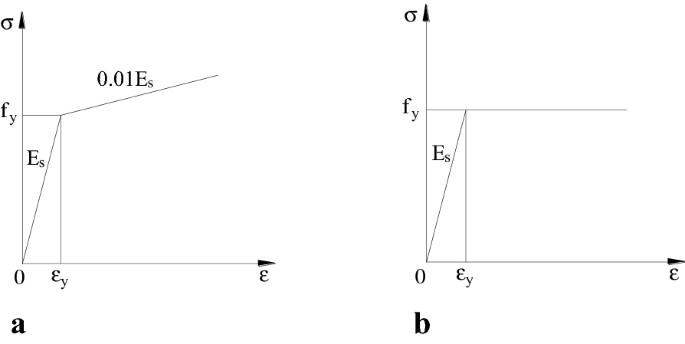
Material modeling of a strengthen elastic–plastic model and b ideal elastic–plastic model.
- 3.
High-Performance Mortar
The mortar is considered to have material properties similar to those of the concrete. However, its numerical values are different from those of the concrete. The parameters obtained from material testing are presented in Table 4.

(3) Element Types and Sizes
The concrete and high-performance mortar are modelled using solid elements (C3D8R, three-dimensional eight-node continuum elements with reduced integration). In order to reduce the complexity of the FE modelling, the vertical rebar in the upper wall and corresponding inserted rebar in the base are regarded as rebars that neglect the strengthening of grouting on the wall. Moreover, because it is subjected to an axial force and a shear force at the connection, it is modelled using beam elements (B31). The other rebars are modelled using two-node truss elements (T3D2).
The element sizes of the concrete in the wall and high-performance mortar are 100 and 50 mm, respectively. Because springs are set with a 50 mm spacing along the unbonded rebar length, and the setting points need to correspond with those in the surrounding concrete, the element size of the concrete in base is 50 mm. Figure 12 shows the FE model of Specimen Z-1. The FE models of the other two specimens are similar to that of Z-1.

Overall configuration of FE model.
5.2 Verification of FE Model
Figure 13 compares the experimental with the simulated results of lateral load–displacement curves for the three specimens. It should be noted that the simulated stiffness is larger than the experimental stiffness. There are two reasons for this. During the simulation, the bonded rebars are embedded in the concrete with no slippage, whereas, in the actual testing, a small slippage inevitably exists between the rebars and concrete. Another reason is that there may have been some slippage between the loading end and the specimen during testing, which led to a smaller experimental stiffness. In addition, it is observed that the experimental peak load is larger than the simulated peak load. However, on the whole, the comparison demonstrates generally good agreement between the experimental and simulated results.

Comparisons of load–displacement curves.
5.3 Parameter Analysis
Only two parameters, namely the unbonded level and axial compression ratio, were considered in the tests. In order to comprehensively study the influence of the unbonded length, unbonded level, and axial compression ratio on the seismic performance of the RHC shear wall, FE models with different parameters were built according to the modelling method in Sect. 5.1, and the results were analysed.
(1) Unbonded Length
Setting the axial compression ratio to 0.2 and the unbonded level to 1 as an example, the unbonded length ranged from 200 to 500 mm, with a 50 mm spacing, as listed in Table 9. Fig 14 shows the influence of the unbonded length on the ductility and energy dissipation of the RHC shear wall.

Effect of unbonded length on a ductility and b energy dissipation.
From Fig. 14, it can be observed that when the axial compression ratio and unbonded level are invariant, the ductility and energy dissipation increase with the unbonded length.
(2) Unbonded Level
Setting the axial compression ratio to 0.2 and the unbonded length to 300 mm as an example, the correspondence of the unbonded rebar distribution in the cross-section and unbonded level (Table 10) are shown in Fig. 15a, b and c shows the influence of the unbonded level on the ductility and energy dissipation of the RHC shear wall.

Effect of unbonded level on b ductility and c energy dissipation. a The rebars in cycles are unbonded, others are bonded.
From Fig. 15, it can be observed that the ductility and energy dissipation of the specimen increase with the unbonded level. However, this increasing trend tends to level off. This is because the ductility and energy dissipation are mainly provided by boundary elements. The effect of the edge rebars is the largest, with the effect of the rebars gradually decreasing from the cross-section’s edge to the middle. Moreover, the increase in the unbonded level represents a gradual increase in the unbonded rebar number from the cross-section’s edge to the middle, as shown in Fig. 15a. Thus, the unbonded level increases, the ductility and energy dissipation increase, but the increasing amplitude decreases.
(3) Axial Compression Ratio
Setting the unbonded length to 300 mm and the unbonded level to 1 as an example, the axial compression ratio ranges from 0.1 to 0.4, with a spacing of 0.05, as listed in Table 11. Fig 16 shows the influence of the axial compression ratio on the bearing capacity of the RHC shear wall.

Effect of axial compression ratio on load–displacement curves.
From Fig. 16, it is showed that when the axial compression ratio increases, the peak load increases. However, the load–displacement curve declines more obviously. This is because there is no cohesive force between the unbonded rebars and concrete, which allows the unbonded rebars’ deformation to increase and the load–displacement curve to rapidly decline under high pressure. Therefore, it is deduced that the unbonded length and unbonded level should not be too large under high pressure.
As the unbonded length and unbonded level obviously also have impacts on the storey drift and drift angle, the design suggestions for the RHC in this paper need to comprehensively consider the effects of the previously discussed factors, which require further study.
6 Conclusions
This paper presented the results of an experimental study and numerical simulation of the seismic performance of a precast shear wall with rabbet-unbonded horizontal connections. Three specimens with various parameters were tested to failure under cyclic quasi-static loading test. A parameter analysis was performed using an ABAQUS FE simulation. Based on the test and numerical results, the following conclusions can be drawn:
- (1)
The final damage phenomena of the three specimens included the yielding of the extreme edge longitudinal rebars in the boundary elements, followed by the crushing of the concrete in the bottom compression and tension zone wall.
- (2)
For the hysteretic behaviour, the hysteresis curve of the specimen with a smaller axial compression ratio was richer and had a larger number of loops. Moreover, the hysteresis curve of the specimen with a larger unbonded level was richer. The trend for the Z-2 and BW-1 skeleton curves was almost consistent with a large initial stiffness. However, Z-1 had a relative small initial stiffness because of a small axial compression ratio.
- (3)
The horizontal bearing capacity of the specimen with a smaller axial compression ratio was smaller. In addition, the bearing capacity of the specimen with a larger unbonded level was slightly smaller.
- (4)
All of the displacements and the ductility factor of the specimen with the smaller axial compression ratio were larger. In addition, all of the displacements and the ductility factor of the specimen with the larger unbonded level were larger. The three specimens had better ductility and deformability.
- (5)
The energy dissipation of the specimen with the smaller axial compression ratio was obviously larger. The energy dissipation of the specimen with the larger unbonded level was larger.
- (6)
The stiffness degradation curve of the specimen with the smaller axial compression ratio declined relatively more slowly. Moreover, in the initial stage, the Z-2 stiffness was smaller than that of BW-1, and in the last stage, the Z-2 stiffness was close to that of BW-1.
- (7)
The parameter analysis using the FE models proved that the ductility and energy dissipation of the RHC shear wall increase with the unbonded length and level. When the axial compression ratio increases, the bearing capacity increases. However, the load–displacement curve declines more obviously. Thus, it is concluded that the unbonded length and unbonded level should not be too large under high pressure, and the design suggestions for the RHC need further research.
Availability of data and material
Not applicable.
References
Buddika, H. A. D. S., & Wijeyewickrema, A. C. (2018). Seismic shear forces in post-tensioned hybrid precast concrete walls. Journal of Structural Engineering, 144(7), 04018086. https://doi.org/10.1061/(ASCE)ST.1943-541X.0002079.
Choi, W., Jang, S. J., & Yun, H. D. (2019). Design properties of insulated precast concrete sandwich panels with composite shear connectors. Composites Part B-Engineering., 157, 36–42.
Dang, X. L., Lv, X. L., Qian, J., & Zhou, Y. (2017). Finite element simulation of self-centering pre-stressed shear walls with horizontal bottom slits. Engineering Mechanics, 34(6), 51–63.
Elsayed, M., Ghrib, F., & Nehdi, M. L. (2018). Experimental and analytical study on precast concrete dowel connections under quasi-static loading. Construction and Building Materials, 168, 692–704.
Gu, A. Q., Zhou, Y., Xiao, Y., Li, Q. W., & Qu, G. (2019). Experimental study and parameter analysis on the seismic performance of self-centering hybrid reinforced concrete shear walls. Soil Dynamics and Earthquake Engineering, 116, 409–420.
Guo, Z. H. (1997). Strength and deformation of concrete-experimental basis and constitutive relation. Bei Jing: Tsinghua University Press.
Guo, T., Wang, L., Xu, Z. K., & Hao, Y. W. (2018). Experimental and numerical investigation of jointed self-centering concrete walls with friction connectors. Journal of Earthquake Engineering, 161(15), 192–206.
Guo, W., Zhai, Z. P., Cui, Y., Yu, Z. W., & Wu, X. L. (2019). Seismic performance assessment of low-rise precast wall panel structure with bolt connections. Engineering Structures, 181, 562–578.
Han, W. L., Zhao, Z. Z., & Qian, J. R. (2019). Global experimental response of a three-story, full-scale precast concrete shear wall structure with reinforcing bars spliced by grouted couplers. PCI Journal, 64(1), 65–80.
Jiang, S. F., Lian, S. H., Zhao, J., Li, X., & Ma, S. L. (2018). Influence of a new form of bolted connection on the mechanical behaviors of a PC shear wall. Applied Sciences-Basel, 8(8), 1381.
Li, J. B., Wang, L., Lu, Z., & Wang, Y. (2018a). Experimental study of L-shaped precast RC shear walls with middle cast-in situ joint. Structural Design of Tall and Special Buildings, 27(6), 1457.
Li, G. C., Wang, Y., Yang, Z. J., & Fang, C. (2018b). Shear behavior of novel T-Stub connection between steel frames and precast reinforced concrete shear walls. International Journal of Steel Structures, 18(1), 115–126.
Liu, C. W., Cao, W. L., Qin, C. J., & Wang, S. M. (2017). Anchorage performance of button-head steel bars in grouted reserved holes in the precast shear wall. Journal of Beijing University of Technology, 43(4), 594–599.
Lu, X. L., Yang, B. Y., & Zhao, B. (2018). Shake-table testing of a self-centering precast reinforced concrete frame with shear walls. Earthquake Engineering and Engineering Vibration, 17(2), 221–233.
Lu, Z., Wang, Y., Li, J. B., & Wang, L. (2019). Experimental study on seismic performance of L-shaped insulated concrete sandwich shear wall with a horizontal seam. Structural Design of Tall and Special Buildings., 28(1), 1551.
Nzabonimpa, J. D., Hong, W. K., & Kim, J. (2017). Nonlinear finite element model for the novel mechanical beam-column joints of precast concrete-based frames. Computers & Structures, 189, 31–48.
Perez, F. J., Mauricio, O. (2018). Verification of a simple model for the lateral-load analysis and design of unbonded post-tensionedprecast concrete walls. PCI Journal, 51–70.
Sorensen, J. H., Hoang, L. C., Olesen, J. F., & Fischer, G. (2017). Test and analysis of a new ductile shear connection design for RC shear walls. Structural Concrete, 18(1), 189–204.
Sun, J., Qiu, H. X., & Jiang, H. B. (2019). Experimental study and associated mechanism analysis of horizontal bolted connections involved in a precast concrete shear wall system. Structural Concrete, 20(1), 282–295.
Twigden, K. M., & Henry, R. S. (2019). Shake table testing of unbonded post-tensioned concrete walls with and without additional energy dissipation. Soil Dynamics and Earthquake Engineering, 119, 375–389.
Twigden, K. M., Sritharan, S., & Henry, R. S. (2017). Cyclic testing of unbonded post-tensioned concrete wall systems with and without supplemental damping. Engineering Structures, 140, 406–420.
Wu, D. Y., Liang, S. T., Guo, Z. X., Zhu, X. J., & Fu, Q. (2016). The development and experimental test of a new pore-forming grouted precast shear wall connector. KSCE Journal of Civil Engineering, 20(4), 1462–1472.
Xiong, C., Chu, M. J., Liu, J. L., & Sun, Z. J. (2018). Shear behavior of precast concrete wall structure based on two-way hollow-core precast panels. Engineering Structures, 176, 74–89.
Xu, L. H., Xiao, S. J., & Li, Z. X. (2018). Hysteretic behavior and parametric studies of a self-centering RC wall with disc spring devices. Soil Dynamics and Earthquake Engineering, 115, 476–488.
Yang, B. Y., & Lu, X. L. (2018). Displacement-based seismic design approach for prestressed precast concrete shear walls and its application. Journal of Earthquake Engineering, 22(10), 1836–1860.
Yi, S. Y. (2018). Seismic behavior of unbonded post-tensioned self-centering concrete shear wall with concealed steel plate brace. Dissertation, Hu Nan University.
Zhu, Z. F., & Guo, Z. X. (2018). Reversed cyclic loading test on emulative hybrid precast concrete shear walls under different vertical loads. KSCE Journal of Civil Engineering, 22(11), 4364–4372.
Zhu, Z. F., Guo, Z. X., & Tang, L. (2018). Experimental study and FEA on seismic performance of new hybrid precast concrete shear walls. China Civil Engineering Journal, 51(3), 36–43.
Acknowledgements
This work was supported by the National Natural Science Foundation for Young Scientists of China (No. 51908336), and China Postdoctoral Science Foundation for General Funding Projects (No. 2019M652301).
Funding
Research grant funded by the National Natural Science Foundation for Young Scientists of China (No. 51908336), and China Postdoctoral Science Foundation for General Funding Projects (No. 2019M652301).
Author information
Authors and Affiliations
Contributions
CFS contributed to writing the manuscript as the principle author. She performed the cyclic quasi-static loading test and numerical simulation research of precast shear wall with rabbet-unbonded horizontal connection. STL and XJZ contributed to guiding the test and numerical simulation. HL contributed to providing the test materials. JMG and GL contributed to construction and installation of specimens. YMS and DYW contributed to collecting the test data. All authors read and approved the final manuscript.
Corresponding author
Ethics declarations
Competing interests
The authors declare that they have no competing interests.
Additional information
Publisher's Note
Springer Nature remains neutral with regard to jurisdictional claims in published maps and institutional affiliations.
Journal information: ISSN 1976-0485 / eISSN 2234-1315
Rights and permissions
Open Access This article is licensed under a Creative Commons Attribution 4.0 International License, which permits use, sharing, adaptation, distribution and reproduction in any medium or format, as long as you give appropriate credit to the original author(s) and the source, provide a link to the Creative Commons licence, and indicate if changes were made. The images or other third party material in this article are included in the article's Creative Commons licence, unless indicated otherwise in a credit line to the material. If material is not included in the article's Creative Commons licence and your intended use is not permitted by statutory regulation or exceeds the permitted use, you will need to obtain permission directly from the copyright holder. To view a copy of this licence, visit http://creativecommons.org/licenses/by/4.0/.
About this article

Cite this article
Sun, Cf., Liang, St., Zhu, Xj. et al. Experimental Study and Numerical Simulation of Precast Shear Wall with Rabbet-Unbonded Horizontal Connection. Int J Concr Struct Mater 14, 6 (2020). https://doi.org/10.1186/s40069-019-0379-3
Received:
Accepted:
Published:
DOI: https://doi.org/10.1186/s40069-019-0379-3