Neutral Higgs boson production at $e^+e^-$ colliders in the complex MSSM: a full one-loop analysis

Abstract

For the search for additional Higgs bosons in the Minimal Supersymmetric Standard Model (MSSM) as well as for future precision analyses in the Higgs sector precise knowledge of their production properties is mandatory. We evaluate the cross sections for the neutral Higgs boson production at $e^+e^-$ colliders in the MSSM with complex parameters (cMSSM). The evaluation is based on a full one-loop calculation of the production mechanism $e^+e^- \rightarrow h_i Z,\, h_i \gamma ,\, h_i h_j$ $(i,j = 1,2,3)$, including soft and hard QED radiation. The dependence of the Higgs boson production cross sections on the relevant cMSSM parameters is analyzed numerically. We find sizable contributions to many cross sections. They are, depending on the production channel, roughly of 10–20 % of the tree-level results, but can go up to 50 % or higher. The full one-loop contributions are important for a future linear $e^+e^-$ collider such as the ILC or CLIC. There are plans to implement the evaluation of the Higgs boson production cross sections into the code FeynHiggs.

1 Introduction

The discovery of a new particle with a mass of about $125 \,\, \mathrm {GeV}$ in the Higgs searches at the Large Hadron Collider (LHC), which has been announced by ATLAS [1] and CMS [2], marks the culmination of an effort that has been ongoing for almost half a century and opens a new era of particle physics. Within the experimental and theoretical uncertainties the properties of the newly discovered particle measured so far are in agreement with a Higgs boson as predicted in the Standard Model (SM) [3].

The identification of the underlying physics of the discovered new particle and the exploration of the mechanism of electroweak symmetry breaking will clearly be a top priority in the future program of particle physics. The most frequently studied realizations are the Higgs mechanism within the SM and within the Minimal Supersymmetric Standard Model (MSSM) [4–7]. Contrary to the case of the SM, in the MSSM two Higgs doublets are required. This results in five physical Higgs bosons instead of the single Higgs boson in the SM. In lowest order these are the light and heavy $\mathcal{CP}$-even Higgs bosons, h and H, the $\mathcal{CP}$-odd Higgs boson, A, and two charged Higgs bosons, $H^\pm$. Within the MSSM with complex parameters (cMSSM), taking higher-order corrections into account, the three neutral Higgs bosons mix and result in the states $h_i$ ($i = 1,2,3$) [8–12]. The Higgs sector of the cMSSM is described at the tree level by two parameters: the mass of the charged Higgs boson, $M_{H^\pm }$, and the ratio of the two vacuum expectation values, $\tan \beta \equiv t_\beta = v_2/v_1$. Often the lightest Higgs boson, $h_1$ is identified [13] with the particle discovered at the LHC [1, 2] with a mass around $\sim 125\,\, \mathrm {GeV}$ [14]. If the mass of the charged Higgs boson is assumed to be larger than $\sim 200\,\, \mathrm {GeV}$ the four additional Higgs bosons are roughly mass degenerate, $M_{H^\pm }\approx m_{h_{2}} \approx m_{h_{3}}$ and referred to as the “heavy Higgs bosons”. Discovering one or more of the additional Higgs bosons would be an unambiguous sign of physics beyond the SM and could yield important information as regards their possible supersymmetric origin.

If supersymmetry (SUSY) is realized in nature and the charged Higgs boson mass is $M_{H^\pm }\lesssim 1.5\,\, \mathrm {TeV}$, then the additional Higgs bosons could be detectable at the LHC [15, 16] (including its high luminosity upgrade, HL-LHC; see Ref. [17] and references therein). This would yield some initial data on the extended Higgs sector. Equally important, the additional Higgs bosons could also be produced at a future linear $e^+e^-$ collider such as the ILC [18–23] or CLIC [23–25]. (Results on the combination of LHC and ILC results can be found in Refs. [26–28].) At an $e^+e^-$ linear collider several production modes for the neutral cMSSM Higgs bosons are possible,

$$\begin{aligned}&e^+e^- \rightarrow h_i Z,\, h_i \gamma ,\, h_i h_j,\, h_i \nu \bar{\nu }, h_i e^+e^-,\, h_i t \bar{t},\, h_i b \bar{b}, \ldots \\&\quad (i,j = 1,2,3). \end{aligned}$$

In the case of a discovery of additional Higgs bosons a subsequent precision measurement of their properties will be crucial to determine their nature and the underlying (SUSY) parameters. In order to yield a sufficient accuracy, one-loop corrections to the various Higgs boson production and decay modes have to be considered. Full one-loop calculations in the cMSSM for various Higgs boson decays to SM fermions, scalar fermions and charginos/neutralinos have been presented over the last years [29–31]. For the decay to SM fermions see also Refs. [32–38]. Decays to (lighter) Higgs bosons have been evaluated at the full one-loop level in the cMSSM in Ref. [29]; see also Refs. [39, 40]. Decays to SM gauge bosons (see also Ref. [41]) can be evaluated to a very high precision using the full SM one-loop result [42–44] combined with the appropriate effective couplings [45]. The full one-loop corrections in the cMSSM listed here together with resummed SUSY corrections have been implemented into the code FeynHiggs [45–50]. Corrections at and beyond the one-loop level in the MSSM with real parameters (rMSSM) are implemented into the code HDECAY [51–53]. Both codes were combined by the LHC Higgs Cross Section Working Group to obtain the most precise evaluation for rMSSM Higgs boson decays to SM particles and decays to lighter Higgs bosons [54].

The most advanced SUSY Higgs boson production calculations at the LHC are available via the code SusHi [55, 56], which are, however, so far restricted to the rMSSM. However, particularly relevant are higher-order corrections also for the Higgs boson production at $e^+e^-$ colliders, where a very high accuracy in the Higgs property determination is anticipated [23]. In this paper we concentrate on the neutral Higgs boson production at $e^+e^-$ colliders in association with a SM gauge boson or another cMSSM Higgs boson, i.e. we calculate $(i,j = 1,2,3)$,

$$\begin{aligned}&\sigma (e^+e^- \rightarrow h_i h_j) , \end{aligned}$$

(1)

$$\begin{aligned}&\sigma (e^+e^- \rightarrow h_i Z) , \end{aligned}$$

(2)

$$\begin{aligned}&\sigma (e^+e^- \rightarrow h_i \gamma ). \end{aligned}$$

(3)

The processes $e^+e^- \rightarrow h_i h_i$ and $e^+e^- \rightarrow h_i \gamma$ are purely loop-induced. The evaluation of the channels (1)–(3) is based on a full one-loop calculation, i.e. including electroweak (EW) corrections, as well as soft and hard QED radiation.

Results for the cross sections (1)–(3) have been obtained over the last two decades. Tree-level calculations for $e^+e^- \rightarrow AH,HZ,Ah$ in the rMSSM have been presented in Ref. [57]. First loop corrections to hZ, hA and AZ production in the rMSSM were published in Refs. [58–60], respectively. A first (nearly) full calculation of the production channels (1) and (2) in the rMSSM was presented in Ref. [61] (leaving out only a detailed evaluation of the initial state radiation).¹ A complete one-loop calculation in the rMSSM of channel (1) with $h_i = h, H$ and $h_j = A$ was presented in Ref. [62]. Unfortunately, only tree-level results were given. A tree-level evaluation of the channels (1) and (2) in the cMSSM was presented in Ref. [63], where higher-order corrections were included via effective couplings. The loop-induced processes (3) with $h_i = h,H,A$ in the rMSSM were published in Ref. [64] and the (also loop-induced) channels (2) and (3) with $h_i = A$ in the cMSSM were published in Ref. [65]. Higher-order corrections to the channels (1) and (2) in the cMSSM were given in Ref. [29], where the third-generation (s)fermion contributions to the production vertex as well as Higgs boson propagator corrections were taken into account. Another full one-loop calculation of $e^+e^- \rightarrow h Z$ was given in Ref. [66], but again restricted to the rMSSM. In Refs. [67, 68] “supersimple” expressions have been derived for the processes $e^+e^- \rightarrow hZ, h\gamma$ in the rMSSM. The production of two equal Higgs bosons in $e^+e^-$ collisions in the rMSSM, where only box diagrams contribute, were presented in Ref. [69] and further discussed in Ref. [70]. Finally, the process $e^+e^- \rightarrow hZ$ with leading corrections in the rMSSM has been computed in Ref. [71]. A numerical comparison with the literature will be given in Sect. 4.

In this paper we present for the first time a full and consistent one-loop calculation for neutral cMSSM Higgs boson production at $e^+e^-$ colliders in association with a SM gauge boson or another cMSSM Higgs boson. We take into account soft and hard QED radiation, collinear divergences and the $\hat{Z}$ factor contributions. In this way we go substantially beyond the existing calculations (see above). In Sect. 2 we very briefly review the renormalization of the relevant sectors of the cMSSM. Details as regards the calculation can be found in Sect. 3. In Sect. 4 various comparisons with results from other groups are given. The numerical results for all production channels (1)–(3) are presented in Sect. 5. The conclusions can be found in Sect. 6. There are plans to implement the evaluation of the production cross sections into the Fortran code FeynHiggs [45–50].

1.1 Prolegomena

We use the following short-hands in this paper:

• FeynTools $\equiv$ FeynArts + FormCalc + LoopTools + FeynHiggs.

• $s_\mathrm {w}\equiv \sin \theta _W$, $c_\mathrm {w}\equiv \cos \theta _W$.

• $s_{\beta - \alpha }\equiv \sin (\beta -\alpha )$, $c_{\beta - \alpha }\equiv \cos (\beta -\alpha )$, $t_\beta \equiv \tan \beta$.

They will be further explained in the text below.

2 The complex MSSM

The cross sections (1)–(3) are calculated at the one-loop level, including soft and hard QED radiation; see the next section. This requires the simultaneous renormalization of the Higgs- and gauge-boson sector as well as the fermion sector of the cMSSM. We give a few relevant details as regards these sectors and their renormalization. More information can be found in Refs. [30, 31, 72–81].

The renormalization of the Higgs and gauge-boson sector follows strictly Ref. [72] and references therein (see especially Ref. [45]). This defines in particular the counterterm $\delta t_\beta$, as well as the counterterms for the Z boson mass, $\delta M_Z^2$, and for the sine of the weak mixing angle, $\delta s_\mathrm {w}$ (with $s_\mathrm {w}= \sqrt{1 - c_\mathrm {w}^2} = \sqrt{1 - M_W^2/M_Z^2}$, where $M_W$ and $M_Z$ denote the W and Z boson masses, respectively).

The renormalization of the fermion sector is described in detail in Ref. [72] and references therein. For simplification we use the ${\overline{\mathrm {DR}}}$ renormalization for all three generations of down-type quarks and leptons, in the notation of Ref. [72]:

$$\begin{aligned}&\texttt {UVMf1[4,\,{\_}] = UVDivergentPart} \\&\quad {\overline{\mathrm {DR}}}\, \text { renormalization for }\, m_d, m_s, m_b \\&\texttt {UVMf1[2,\,{\_}] = UVDivergentPart} \\&\quad {\overline{\mathrm {DR}}}\, \text { renormalization for }\, m_e, m_\mu , m_\tau . \end{aligned}$$

3 Calculation of diagrams

In this section we give some details as regards the calculation of the tree-level and higher-order corrections to the production of Higgs bosons in $e^+e^-$ collisions. The diagrams and corresponding amplitudes have been obtained with FeynArts (version 3.9) [82–84], using the MSSM model file (including the MSSM counterterms) of Ref. [72]. The further evaluation has been performed with FormCalc (version 8.4) and LoopTools (version 2.12) [85]. The Higgs sector quantities (masses, mixings, $\hat{Z}$ factors, etc.) have been evaluated using FeynHiggs [45–50] (version 2.11.0).

3.1 Contributing diagrams

Sample diagrams for the process $e^+e^- \rightarrow h_i h_j$ ($i,j = 1,2,3$) are shown in Fig. 1, for the process $e^+e^- \rightarrow h_i Z$ ($i = 1,2,3$) in Fig. 2, and for the process $e^+e^- \rightarrow h_i \gamma$ $(i = 1,2,3$) in Fig. 3. Not shown are the diagrams for real (hard and soft) photon radiation. They are obtained from the corresponding tree-level diagrams by attaching a photon to the electrons/positrons. The internal particles in the generically depicted diagrams in Figs. 1, 2, and 3 are labeled as follows: F can be a SM fermion f, chargino $\tilde{\chi }_{c}^\pm$ or neutralino $\tilde{\chi }_{n}^0$; S can be a sfermion ${\tilde{f}}_s$ or a Higgs (Goldstone) boson $h_i, H^\pm$ ($G, G^\pm$); U denotes the ghosts $u_V$; V can be a photon $\gamma$ or a massive SM gauge boson, Z or $W^\pm$. We have neglected all electron–Higgs couplings via the FeynArts command [82–84]

$$\begin{aligned} \texttt {Restrictions -> {NoElectronHCoupling}} \end{aligned}$$

and terms proportional to the electron mass $\texttt {ME}$ (and the squared electron mass $\texttt {ME2}$) via the FormCalc command [85]

$$\begin{aligned} \texttt {Neglect[ME] = Neglect[ME2] = 0} \end{aligned}$$

which allows FormCalc to replace $\texttt {ME}$ by zero whenever this is safe, i.e. except when it appears in negative powers or in loop integrals. We have verified numerically that these contributions are indeed totally negligible. For internally appearing Higgs bosons no higher-order corrections to their masses or couplings are taken into account; these corrections would correspond to effects beyond one-loop order.² For external Higgs bosons, as discussed in Ref. [45], the appropriate $\hat{Z}$ factors are applied and on-shell (OS) masses (including higher-order corrections) are used [45], obtained with FeynHiggs [45–50].

Fig. 1

Generic tree, self-energy, vertex, box, and counterterm diagrams for the process $e^+e^- \rightarrow h_i h_j$ ($i,j = 1,2,3$). F can be a SM fermion, chargino or neutralino; S can be a sfermion or a Higgs/Goldstone boson; V can be a $\gamma$, Z or $W^\pm$. It should be noted that electron–Higgs couplings are neglected

Fig. 2

Generic tree, self-energy, vertex, box, and counterterm diagrams for the process $e^+e^- \rightarrow h_i Z$ ($i = 1,2,3$). F can be a SM fermion, chargino or neutralino; S can be a sfermion or a Higgs/Goldstone boson; V can be a $\gamma$, Z or $W^\pm$. It should be noted that electron–Higgs couplings are neglected

Fig. 3

Generic vertex, box, and counterterm diagrams for the (loop-induced) process $e^+e^- \rightarrow h_i \gamma$ ($i = 1,2,3$). F can be a SM fermion, chargino or neutralino; S can be a sfermion or a Higgs/Goldstone boson; V can be a $\gamma$, Z or $W^\pm$. It should be noted that electron–Higgs couplings are neglected

Also not shown are the diagrams with a Z/Goldstone–Higgs boson self-energy contribution on the external Higgs boson leg. They appear in $e^+e^- \rightarrow h_i h_j$, with a Z / G–$h_{i,j}$ transition and have been calculated explicitly as far as they are not proportional to the electron mass. It should be noted that for the process $e^+e^- \rightarrow h_i Z$ all these contributions are proportional to the electron mass and have consistently be neglected.

Fig. 4

Phase space slicing method. The different contributions to the loop corrections $\delta \sigma (e^+e^- \rightarrow h_1 Z)$ at $\sqrt{s} = 500\,\, \mathrm {GeV}$ with fixed $\Delta \theta /\text {rad} = 10^{-2}$ (upper plot) and fixed $\Delta E/E = 10^{-3}$ (lower plot)

Furthermore, in general, in Figs. 1, 2, and 3 we have omitted diagrams with self-energy type corrections of external (on-shell) particles. While the contributions from the real parts of the loop functions are taken into account via the renormalization constants defined by OS renormalization conditions, the contributions coming from the imaginary part of the loop functions can result in an additional (real) correction if multiplied by complex parameters. In the analytical and numerical evaluation, these diagrams have been taken into account via the prescription described in Ref. [72].

Within our one-loop calculation we neglect finite width effects that can help to cure threshold singularities. Consequently, in the close vicinity of those thresholds our calculation does not give a reliable result. Switching to a complex mass scheme [86] would be another possibility to cure this problem, but its application is beyond the scope of our paper.

For completeness we show here the tree-level cross section formulas:

$$\begin{aligned}&\sigma _{\text {tree}}(e^+e^- \rightarrow h_i h_j) \nonumber \\&\quad = \frac{\pi \, \alpha ^2}{96\, s} \left( \frac{8\, s_\mathrm {w}^4 - 4\, s_\mathrm {w}^2 + 1}{s_\mathrm {w}^4\,c_\mathrm {w}^4}\right) \frac{\lambda ^{3/2}(1,m_{h_{i}}^2/s,m_{h_{j}}^2/s)}{(1-M_Z^2/s)^2} \nonumber \\&\quad \quad \times | \hat{Z}_{j3} (c_{\beta - \alpha }\, \hat{Z}_{i1} - s_{\beta - \alpha }\, \hat{Z}_{i2})\nonumber \\&\quad \quad - \hat{Z}_{i3} (c_{\beta - \alpha }\, \hat{Z}_{j1} - s_{\beta - \alpha }\, \hat{Z}_{j2}) |^2, \end{aligned}$$

(4)

$$\begin{aligned}&\sigma _{\text {tree}}(e^+e^- \rightarrow h_i Z) \nonumber \\&\quad =\frac{\pi \, \alpha ^2}{96\, s} \left( \frac{8\, s_\mathrm {w}^4 - 4\, s_\mathrm {w}^2 + 1}{s_\mathrm {w}^4\, c_\mathrm {w}^4} \right) \,\frac{\lambda (1,m_{h_{i}}^2/s,M_Z^2/s) + 12\,M_Z^2/s }{(1-M_Z^2/s)^2}\, \nonumber \\&\quad \quad \times \lambda ^{1/2}(1,m_{h_{i}}^2/s,M_Z^2/s)\, | s_{\beta - \alpha }\, \hat{Z}_{i1} + c_{\beta - \alpha }\, \hat{Z}_{i2} |^2, \end{aligned}$$

(5)

where $i,j = 1,2,3$ ($i \ne j$) and $\lambda (x,y,z) = (x - y - z)^2 - 4yz$ denotes the two-body phase space function. The Z-factor matrix is given by $\hat{Z}_{ij} \equiv \texttt {ZHiggs[ i ,\, j ]}$, see Ref. [72] (and Ref. [45]) and is calculated by FeynHiggs.

3.2 Ultraviolet divergences

As regularization scheme for the UV divergences we have used constrained differential renormalization [87], which has been shown to be equivalent to dimensional reduction [88, 89] at the one-loop level [85]. Thus the employed regularization scheme preserves SUSY [90, 91] and guarantees that the SUSY relations are kept intact, e.g. that the gauge couplings of the SM vertices and the Yukawa couplings of the corresponding SUSY vertices also coincide to one-loop order in the SUSY limit. Therefore no additional shifts, which might occur when using a different regularization scheme, arise. All UV divergences cancel in the final result.³

3.3 Infrared divergences

Soft photon emission implies numerical problems in the phase space integration of radiative processes. The phase space integral diverges in the soft energy region where the photon momentum becomes very small, leading to infrared (IR) singularities. Therefore the IR divergences from diagrams with an internal photon have to cancel with the ones from the corresponding real soft radiation. We have included the soft photon contribution via the code already implemented in FormCalc following the description given in Ref. [92]. The IR divergences arising from the diagrams involving a photon are regularized by introducing a photon mass parameter, $\lambda$. All IR divergences, i.e. all divergences in the limit $\lambda \rightarrow 0$, cancel once virtual and real diagrams for one process are added. We have (numerically) checked that our results do not depend on $\lambda$.

We have also numerically checked that our results do not depend on $\Delta E = \delta _s E = \delta _s \sqrt{s}/2$ defining the energy cut that separates the soft from the hard radiation. As one can see from the example in the upper plot of Fig. 4 this holds for several orders of magnitude. Our numerical results below have been obtained for fixed $\delta _s = 10^{-3}$.

3.4 Collinear divergences

Numerical problems in the phase space integration of the radiative process arise also through collinear photon emission. Mass singularities emerge as a consequence of the collinear photon emission off massless particles. But already very light particles (such as e.g. electrons) can produce numerical instabilities.

There are several methods for the treatment of collinear singularities. In the following, we give a very brief description of the so-called phase space slicing (PSS) method [93–96], which we adopted. The treatment of collinear divergences is not (yet) implemented in FormCalc, and therefore we have developed and implemented the code necessary for the evaluation of collinear contributions.

Table 1 Comparison of the one-loop corrected Higgs production cross sections (in fb) with FeynHiggsXS at $\sqrt{s} = 1000\,\, \mathrm {GeV}$ and $M_{H^\pm }= 310.86$ and higgsmix = 3 as input in FeynHiggs. FeynTools: $m_h = 123.17\,\, \mathrm {GeV}$, $m_H = 300.00\,\, \mathrm {GeV}$, $m_{A} = 301.70\,\, \mathrm {GeV}$. FeynHiggsXS: $m_h = 118.68\,\, \mathrm {GeV}$, $m_H = 301.84\,\, \mathrm {GeV}$, $m_{A} = 300.00\,\, \mathrm {GeV}$

In the PSS method, the phase space is divided into regions where the integrand is finite (numerically stable) and regions where it is divergent (or numerically unstable). In the stable regions the integration is performed numerically, whereas in the unstable regions it is carried out (semi-) analytically using approximations for the collinear photon emission.

The collinear part is constrained by the angular cut-off parameter $\Delta \theta$, imposed on the angle between the photon and the (in our case initial state) electron/positron.

The differential cross section for the collinear photon radiation off the initial state $e^+e^-$ pair corresponds to a convolution

$$\begin{aligned} \text {d}\sigma _{\text {coll}}(s)= & {} \frac{\alpha }{\pi } \int _0^{1-\delta _s} \text {d}z\, \text {d}\sigma _{\text {tree}}(\sqrt{z s})\nonumber \\&\times \left\{ \left[ 2\, \ln \left( \frac{\Delta \theta \sqrt{s}}{2\, m_e} \right) - 1 \right] P_{ee}(z) + 1 - z \right\} , \end{aligned}$$

(6)

with $P_{ee}(z) = (1 + z^2)/(1 - z)$ denoting the splitting function of a photon from the initial $e^+e^-$ pair. The electron momentum is reduced (because of the radiated photon) by the fraction z such that the center-of-mass frame of the hard process receives a boost. The integration over all possible factors z is constrained by the soft cut-off $\delta _s = \Delta E/E$, to prevent over-counting in the soft energy region.

We have (numerically) checked that our results do not depend on $\Delta \theta$ over several orders of magnitude; see the example in the lower plot of Fig. 4. Our numerical results below have been obtained for fixed $\Delta \theta /\text {rad} = 10^{-2}$.

Table 2 MSSM default parameters for the numerical investigation; all parameters (except of $t_\beta$) are in GeV (calculated masses are rounded to 1 MeV). The values for the trilinear sfermion Higgs couplings, $A_{t,b,\tau }$ are chosen such that charge- and/or color-breaking minima are avoided [100–106], and $A_{b,\tau }$ are chosen to be real. It should be noted that for the first and second generation of sfermions we chose instead $A_f = 0$, $M_{\tilde{Q}, \tilde{U}, \tilde{D}} = 1500\,\, \mathrm {GeV}$ and $M_{\tilde{L}, \tilde{E}} = 500\,\, \mathrm {GeV}$

The one-loop corrections of the differential cross section are decomposed into the virtual, soft, hard, and collinear parts as follows:

$$\begin{aligned} \text {d}\sigma _{\text {loop}}= & {} \text {d}\sigma _{\text {virt}}(\lambda ) + \text {d}\sigma _{\text {soft}}(\lambda , \Delta E) \nonumber \\&+\,\text {d}\sigma _{\text {hard}}(\Delta E, \Delta \theta ) + \text {d}\sigma _{\text {coll}}(\Delta E, \Delta \theta ). \end{aligned}$$

(7)

The hard and collinear parts have been calculated via the Monte Carlo integration algorithm Vegas as implemented in the CUBA library [97] as part of FormCalc.

4 Comparisons

In this section we present the comparisons with results from other groups in the literature for neutral Higgs boson production in $e^+e^-$ collisions. Most of these comparisons were restricted to the MSSM with real parameters. The level of agreement of such comparisons (at one-loop order) depends on the correct transformation of the input parameters from our renormalization scheme into the schemes used in the respective literature, as well as on the differences in the employed renormalization schemes as such. In view of the non-trivial conversions and the large number of comparisons such transformations and/or change of our renormalization prescription is beyond the scope of our paper.

• In Ref. [57] the processes $e^+e^- \rightarrow AH,HZ,Ah$ have been calculated in the rMSSM at tree level. As input parameters we used their parameters as far as possible. For the comparison with Ref. [57] we successfully reproduced their upper Fig. 2.

• A numerical comparison with the program FeynHiggsXS [61] can be found in Table 1. We have neglected the initial state radiation and diagrams with photon exchange, as done in Ref. [61]. In Table 1 “self”, “self+vert” and “full” denote the inclusion of only self-energy corrections, self-energy plus vertex corrections or the full calculation including box diagrams. The comparison for the production of the light Higgs boson is rather difficult, due to the different FeynHiggs versions. As input parameters we used our scenario $\mathcal S$; see Table 2 below. (We had to change only $A_{t,b,\tau }$ to $A_{t,b} = 1500$ and $A_{\tau } = 0$ to be in accordance with the input options of FeynHiggsXS.) It can be observed that the level of agreement for the “self+vert” calculation is mostly at the level of 5 % or better. However, the box contributions appear to go in the opposite direction for the first three cross sections in the two calculations. This hints toward a problem in the box contributions in Ref. [61], where the box contributions were obtained independently from the rest of the loop corrections (see also the comparison with Ref. [58] below), whereas using FeynTools all corrections are evaluated together in an automated way. It should be noted that a self-consistent check with the program FeynHiggsXS gave good agreement with Ref. [61] as expected (with tiny differences due to slightly different SM input parameters).

• In Ref. [62] the processes $e^+e^- \rightarrow HA, hA$ (and $e^+e^- \rightarrow H^+ H^-$) have been calculated in the rMSSM. Unfortunately, in Ref. [62] the numerical evaluation (shown in their Fig. 2) are only tree-level results, although the paper deals with the respective one-loop corrections. For the comparison with Ref. [62] we successfully reproduced their lower Fig. 2.

• In Ref. [63] a tree-level evaluation of the channels (1) and (2) in the cMSSM was presented, where higher-order corrections were included via ($\mathcal{CP}$ violating) effective couplings. Unfortunately, no numbers are given in Ref. [63], but only two-dimensional parameter scan plots, which we could not reasonably compare to our results. Consequently we omitted a comparison with Ref. [63].

• We performed a comparison with Ref. [29] for $e^+ e^- \rightarrow h_i Z, h_i h_j$ ($i,j = 1,2,3$) at $\mathcal{O}(\alpha )$ in the cMSSM. In Ref. [29] only self-energy and vertex corrections involving $t, {\tilde{t}}, b, \tilde{b}$ were included, and the numerical evaluation was performed in the CPX scenario [98] (with $M_{H^\pm }$ chosen to yield $m_{h_{1}} = 40\,\, \mathrm {GeV}$) which is extremely sensitive to the chosen input parameters. Nevertheless, using their input parameters as far as possible, we found qualitative agreement for $t_\beta < 15$ with their Fig. 20. For larger $t_\beta$ values the CPX scenario appears to be too sensitive to small deviations in the input parameters, and the agreement worsened.

• $e^+e^- \rightarrow hZ$ at the full one-loop level (including hard and soft photon bremsstrahlung, as well as ${\hat{\mathbf {Z}}}$ matrix contributions) has been analyzed in Ref. [66]. While complex parameters in this work are mentioned, all formulas and numerical examples only concern the rMSSM. They also used FeynArts, FormCalc and LoopTools to generate and simplify their code. Unfortunately no numbers are given in Ref. [66], but only two-dimensional parameter scan plots, which we could not reasonably compare to our results. Consequently, we omitted a comparison with Ref. [66].

• In Refs. [67, 68] “supersimple” expressions have been derived for the processes $e^+e^- \rightarrow hZ, h\gamma$ in the rMSSM. We successfully reproduced Fig. 4 (right panels) of Ref. [67] in the upper plots of our Fig. 5 and Fig. 5 (right panels) of Ref. [68] in the lower plots of our Fig. 5. As input parameters we used their (SUSY) parameter set S1. The small differences in the differential cross sections are caused by the SM input parameters (where we have used our parameters; see Sect. 5.1 below) and the slightly different renormalization schemes and treatment of the Higgs boson masses.

• The Higgsstrahlung process $e^+e^- \rightarrow hZ$ with the expected leading corrections in “Natural SUSY” models [i.e. a one-loop calculation with third-generation (s)quarks] has been computed in Ref. [71] for real parameters. This work also used FeynArts, FormCalc, and LoopTools to generate and simplify their code. Unfortunately, again no numbers are given in Ref. [71], but mostly two-dimensional parameter scan plots, which we could not reasonably compare to our results. Only in the left plot of their Fig. 4 they show (fractional) corrections to the Higgsstrahlung cross section. However, the MSSM input parameters are not given in detail, rendering a comparison again impossible.

• In Ref. [58] the box contributions to the processes $e^+e^- \rightarrow hZ,hA$ were computed. We used their input parameters as far as possible and reproduced Figs. 5 and 8 (solid lines, “box”) of Ref. [58] in our Fig. 6. The small differences are due to slightly different SM input parameters. However, we disagree in the sign of the box contributions in $e^+e^- \rightarrow hA$, except for the sneutrino loops. Consequently, the sign difference of the full box contributions w.r.t. our result depends on the choice of the MSSM parameters. It should be noted that the code of Ref. [58] is also part of the code from Ref. [59] (see the next item) and Ref. [61].

  Fig. 5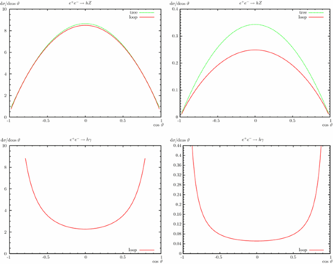

  

  $\sigma (e^+e^- \rightarrow h Z, h \gamma )$. The left (right) plots show the differential cross section with $\sqrt{s} = 1\,\, \mathrm {TeV}$ ($5\,\, \mathrm {TeV}$) and $\cos \vartheta$ varied. Upper row tree-level and one-loop corrected differential cross sections (in fb) are shown with parameters chosen according to S1 of Ref. [67]. Lower row loop-induced differential cross sections (in ab) are shown with parameters chosen according to S1 of Ref. [68]

  Fig. 6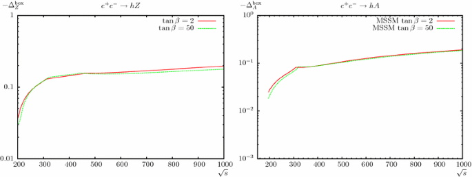

  

  $\sigma (e^+e^- \rightarrow h Z, h A)$. The relative box contributions are shown with MSSM parameters chosen according to Ref. [58]. The left (right) plot shows the cross section for $e^+e^- \rightarrow h Z$ ($e^+e^- \rightarrow h A$) with $\sqrt{s}$ varied

  Fig. 7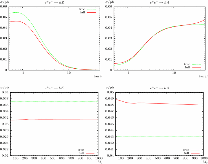

  

  $\sigma (e^+e^- \rightarrow h Z, h A)$. One-loop corrected cross sections (in fb) are shown with parameters chosen according to Ref. [59]. The upper left (right) plot shows the cross section for $e^+e^- \rightarrow h Z$ ($e^+e^- \rightarrow h A$) with $t_\beta$ varied at $\sqrt{s} = 500\,\, \mathrm {GeV}$. The lower left (right) plot shows the cross section for $e^+e^- \rightarrow h Z$ ($e^+e^- \rightarrow h A$) with $M_2$ varied at $\sqrt{s} = 500\,\, \mathrm {GeV}$

  Fig. 8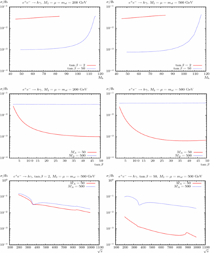

  

  $\sigma (e^+e^- \rightarrow A Z)$. Loop-induced cross sections (in fb) are shown with parameters chosen according to Ref. [64]. The upper plots show the cross section with $M_A$ varied at $\sqrt{s} = 500$. The lower plots show the cross section for $\sqrt{s}$ varied

  Fig. 9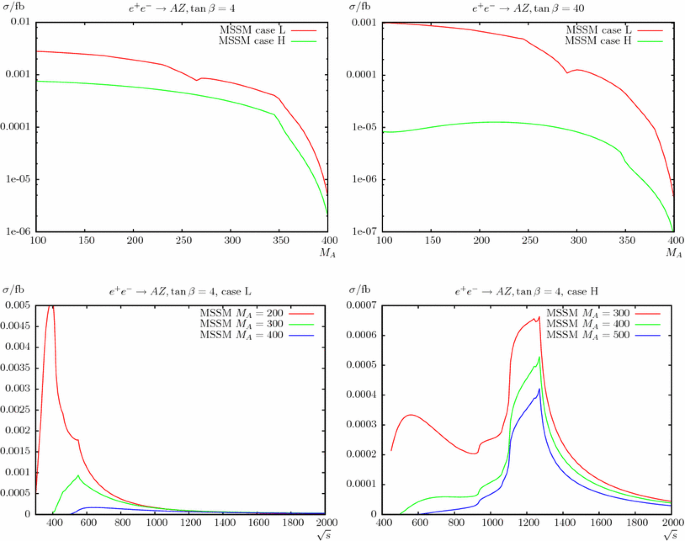

  

  $\sigma (e^+e^- \rightarrow h \gamma )$. Loop-induced cross sections (in fb) are shown with parameters chosen according to Ref. [60]. The upper plots show the cross section with $M_h$ varied at $\sqrt{s} = 500$. The middle plots show the cross section for $t_\beta$ varied at $\sqrt{s} = 500$. The lower plots show the cross section for $\sqrt{s}$ varied

• In Ref. [59] the processes $e^+e^- \rightarrow hZ, hA$ are computed within a complete one-loop calculation. Only the QED (including photon bremsstrahlung) has been neglected. We used their input parameters as far as possible and (more or less successfully) reproduced Figs. 5 and 6 (upper rows, solid lines) of Ref. [59] qualitatively in our Fig. 7. Smaller differences are mainly due to different Higgs boson masses and the use of Higgs boson wave function corrections in Ref. [59], while we used an effective mixing angle $\alpha _{\text {eff}}$. In order to facilitate the comparison we used the same simple formulas for our Higgs boson masses and $\alpha _{\text {eff}}$ as in their Eqs. (4)–(7). Therefore our $\sigma _{\text {tree}}$ correspond rather to their $\sigma ^{\epsilon }$ and our $\sigma _{\text {full}}$ rather to their $\sigma ^{\text {FDC}}$. The larger differences in the loop corrections of $e^+e^- \rightarrow hA$ (right plots of our Fig. 7) are due to the different sign of the leading box contributions of Ref. [59]; see also the latter item. It should be noted that the code of Ref. [59] is also part of the code from Ref. [61]. Using FeynHiggsXS with the input parameters of Ref. [59] (as far as possible) gave also only qualitative agreement with the Figs. of Ref. [59].

• In Ref. [64] the loop-induced processes $e^+e^- \rightarrow h\gamma , H\gamma , A\gamma$ have been computed. We used the same simple formulas for our Higgs boson masses and $\alpha _{\text {eff}}$ as in their Eqs. (3.48)–(3.50). We also used their input parameters as far as possible, but unfortunately they forgot to specify the trilinear parameters $A_f$. Therefore we chose arbitrarily $A_f = 0$ for our comparison. In view of this problem the comparison is acceptable; see our Fig. 8 vs. Figs. 4, 5 and 7 of Ref. [64]. It should be noted that the code of Ref. [64] is also part of the code from Refs. [59, 61].

• In Ref. [60] the loop-induced process $e^+e^- \rightarrow A Z$ has been computed in the rMSSM using FeynArts, FormCalc and LoopTools. We used their input parameters (as far as possible) and are in good agreement with their Figs. 2 and 4; see our Fig. 9. We only significantly differ quantitatively for $t_\beta = 4$ in combination with their case L (which denotes light SUSY particles). However, we could not find why in this particular case the comparison failed.

• In Ref. [65] the loop-induced processes $e^+e^- \rightarrow A\gamma , A Z$ have been computed in the cMSSM using also FeynArts, FormCalc and LoopTools. We used their input parameters and are in good qualitative agreement with their Figs. 3 and 5. But again we differ quantitative significantly by roughly a factor 1.3 (1.7) in $e^+e^- \rightarrow A\gamma$ ($e^+e^- \rightarrow A Z$). As in Ref. [60] (see above) this is due to the low $t_\beta$ and SUSY masses used in Ref. [65]. Unfortunately the code of Ref. [65] is no longer available, making further investigations impossible. But we repeated successfully (9 digits agreement) our calculations with the older versions of FeynArts (i.e. MSSM model files) and FormCalc as they were used in Ref. [65], i.e. the different versions of FeynArts and FormCalc can be excluded as a reason for this discrepancy.

A final comment is in order. We argue that the problems in the comparison with Ref. [61] (i.e. FeynHiggsXS), Refs. [59, 64] are due to the fact that all three papers are based (effectively) on the same calculation/source, where we discussed the differences in particular in the sign of some box contributions. Consequently, these three papers should be considered as one rather than three independent comparisons, and thus do not disprove the reliability of our calculation. It should also be kept in mind that our calculational method/code has already been successfully tested and compared with quite a few other programs; see Refs. [30, 31, 72–80].

5 Numerical analysis

In this section we present our numerical analysis of neutral Higgs boson production at $e^+e^-$ colliders in the cMSSM. In the various figures below we show the cross sections at the tree level (“tree”) and at the full one-loop level (“full”). In case of extremely small tree-level cross sections we also show results including the corresponding purely loop-induced contributions (“loop”). These leading two-loop contributions are $\propto |\mathcal{M}_{\text {1-loop}}|^2$, where $\mathcal{M}_{\text {1-loop}}$ denotes the one-loop matrix element of the appropriate process.

5.1 Parameter settings

The renormalization scale $\mu _R$ has been set to the center-of-mass energy, $\sqrt{s}$. The SM parameters are chosen as follows; see also [99]:

• Fermion masses (on-shell masses, if not indicated differently):

  $$\begin{aligned} \begin{array}{l@{\quad }l} m_e = 0.510998928\,\, \mathrm {MeV}, &{} m_{\nu _e} = 0, \\ m_\mu = 105.65837515\,\, \mathrm {MeV}, &{} m_{\nu _{\mu }} = 0, \\ m_\tau = 1776.82\,\, \mathrm {MeV}, &{} m_{\nu _{\tau }} = 0, \\ m_u = 68.7\,\, \mathrm {MeV}, &{} m_d = 68.7\,\, \mathrm {MeV}, \\ m_c = 1.275\,\, \mathrm {GeV}, &{} m_s = 95.0\,\, \mathrm {MeV}, \\ m_t = 173.21\,\, \mathrm {GeV}, &{} m_b = 4.18\,\, \mathrm {GeV}. \end{array} \end{aligned}$$

  (8)

  According to Ref. [99], $m_s$ is an estimate of a so-called “current quark mass” in the $\overline{\mathrm {MS}}$ scheme at the scale $\mu \approx 2\,\, \mathrm {GeV}$. $m_c \equiv m_c(m_c)$ and $m_b \equiv m_b(m_b)$ are the “running” masses in the $\overline{\mathrm {MS}}$ scheme. $m_u$ and $m_d$ are effective parameters, calculated through the hadronic contributions to

  $$\begin{aligned} \Delta \alpha _{\text {had}}^{(5)}(M_Z)&= \frac{\alpha }{\pi }\sum _{f = u,c,d,s,b} Q_f^2 \left( \ln \frac{M_Z^2}{m_f^2} - \frac{5}{3}\right) \nonumber \\&\approx 0.027723. \end{aligned}$$

  (9)

• Gauge boson masses:

  $$\begin{aligned} M_Z = 91.1876\,\, \mathrm {GeV}, \quad M_W = 80.385\,\, \mathrm {GeV}. \end{aligned}$$

  (10)

• Coupling constant:

  $$\begin{aligned} \alpha (0) = 1/137.0359895. \end{aligned}$$

  (11)

The Higgs sector quantities (masses, mixings, $\hat{Z}$ factors, etc.) have been evaluated using FeynHiggs (version 2.11.0) [45–50].

The SUSY parameters are chosen according to the scenario $\mathcal S$, shown in Table 2, unless otherwise noted. This scenario constitutes a viable scenario for the various cMSSM Higgs production modes, i.e. not picking specific parameters for each cross section. The only variation will be the choice of $\sqrt{s} = 500\,\, \mathrm {GeV}$ for production cross sections involving the light Higgs boson.⁴ This will be clearly indicated below. We do not strictly demand that the lightest Higgs boson has a mass around $\sim 125\,\, \mathrm {GeV}$, although for most of the parameter space this is given. We will show the variation with $\sqrt{s}$, $M_{H^\pm }$, $t_\beta$ and $\varphi _{A_t}$, the phase of $A_t$.

Concerning the complex parameters, some more comments are in order. No complex parameter enters into the tree-level production cross sections. Therefore, the largest effects are expected from the complex phases entering via the $t/{\tilde{t}}$ sector, i.e. from $\varphi _{A_t}$, motivating our choice of $\varphi _{A_t}$ as parameter to be varied. Here the following should be kept in mind. When performing an analysis involving complex parameters it should be noted that the results for physical observables are affected only by certain combinations of the complex phases of the parameters $\mu$, the trilinear couplings $A_f$ and the gaugino mass parameters $M_{1,2,3}$ [108, 109]. It is possible, for instance, to rotate the phase $\varphi _{M_2}$ away. Experimental constraints on the (combinations of) complex phases arise, in particular, from their contributions to electric dipole moments of the electron and the neutron (see Refs. [110–112] and references therein), of the deuteron [113] and of heavy quarks [114, 115]. While SM contributions enter only at the three-loop level, due to its complex phases the MSSM can contribute already at one-loop order. Large phases in the first two generations of sfermions can only be accommodated if these generations are assumed to be very heavy [116, 117] or large cancellations occur [118–120]; see, however, the discussion in Ref. [121]. A review can be found in Ref. [122]. Accordingly (using the convention that $\varphi _{M_2}= 0$, as done in this paper), in particular, the phase $\varphi _{\mu }$ is tightly constrained [123], while the bounds on the phases of the third-generation trilinear couplings are much weaker. Setting $\varphi _{\mu }= 0$ and $\varphi _{A_{f \ne t}} = 0$ leaves us with $\varphi _{A_t}$ as the only complex valued parameter.

Fig. 10

$\sigma (e^+e^- \rightarrow h_1 h_2)$. Tree-level and full one-loop corrected cross sections are shown with parameters chosen according to $\mathcal S$; see Table 2. The upper plots show the cross sections with $\sqrt{s}$ (left) and $M_{H^\pm }$ (right) varied; the lower plots show $t_\beta$ (left) and $\varphi _{A_t}$ (right) varied

Since now the complex trilinear coupling $A_t$ can appear in the couplings, contributions from absorptive parts of self-energy type corrections on external legs can arise. The corresponding formulas for an inclusion of these absorptive contributions via finite wave function correction factors can be found in Refs. [72, 75].

Fig. 11

$\sigma (e^+e^- \rightarrow h_2 h_3)$. Tree-level and full one-loop corrected cross sections are shown with parameters chosen according to $\mathcal S$; see Table 2. The upper plots show the cross sections with $\sqrt{s}$ (left) and $M_{H^\pm }$ (right) varied; the lower plots show $t_\beta$ (left) and $\varphi _{A_t}$ (right) varied

Fig. 12

$\sigma (e^+e^- \rightarrow h_1 h_1)$. Loop-induced (i.e. leading two-loop corrected) cross sections are shown with parameters chosen according to $\mathcal S$ (see Table 2), but with $\sqrt{s} = 500\,\, \mathrm {GeV}$. The upper plots show the cross sections with $\sqrt{s}$ (left) and $M_{H^\pm }$ (right) varied; the lower plots show $t_\beta$ (left) and $\varphi _{A_t}$ (right) varied

Fig. 13

$\sigma (e^+e^- \rightarrow h_2 h_2, h_3 h_3)$. Loop-induced (i.e. leading two-loop corrected) cross sections are shown with parameters chosen according to $\mathcal S$; see Table 2. The upper plots show the cross sections with $\sqrt{s}$ (left) and $M_{H^\pm }$ (right) varied; the lower plots show $t_\beta$ (left) and $\varphi _{A_t}$ (right) varied

The numerical results shown in the next subsections are of course dependent on the choice of the SUSY parameters. Nevertheless, they give an idea of the relevance of the full one-loop corrections.

5.2 Full one-loop results for varying $\sqrt{s}$, $M_{H^\pm }$, $t_\beta$, and $\varphi _{A_t}$

The results shown in this and the following subsections consist of “tree”, which denotes the tree-level value and of “full”, which is the cross section including all one-loop corrections as described in Sect. 3.

We begin the numerical analysis with the cross sections of $e^+e^- \rightarrow h_i h_j$ ($i,j = 1,2,3$) evaluated as a function of $\sqrt{s}$ (up to $3\,\, \mathrm {TeV}$, shown in the upper left plot of the respective figures), $M_{H^\pm }$ (starting at $M_{H^\pm }= 160\,\, \mathrm {GeV}$ up to $M_{H^\pm }= 500\,\, \mathrm {GeV}$, shown in the upper right plots), $t_\beta$ (from 4 to 50, lower left plots) and $\varphi _{A_t}$ (between $0^{\circ }$ and $360^{\circ }$, lower right plots). Then we turn to the processes $e^+e^- \rightarrow h_i Z$ and $e^+e^- \rightarrow h_i \gamma$ ($i = 1,2,3$). All these processes are of particular interest for ILC and CLIC analyses [18–22, 24, 25] (as emphasized in Sect. 1).

5.2.1 The process $e^+e^- \rightarrow h_i h_j$

We start our analysis with the production modes $e^+e^- \rightarrow h_i h_j$ ($i,j = 1,2,3$). Results are shown in the Figs. 10, 11, 12, and 13. It should be noted that there are no hHZ couplings in the rMSSM (see Ref. [124]). For real parameters this leads to vanishing tree-level cross sections if $h_i \sim h$ and $h_j \sim H$ (or vice versa). Furthermore there are no hhZ, HHZ, and AAZ couplings in the rMSSM, but also in the complex case the tree couplings $h_i h_i Z$ ($i = 1,2,3$) are exactly zero (see Ref. [124]). In the following analysis $e^+ e^- \rightarrow h_i h_i$ ($i = 1,2,3$) are loop induced via (only) box diagrams and therefore $\propto |\mathcal{M}_{\text {1-loop}}|^2$.

We begin with the process $e^+e^- \rightarrow h_1 h_2$ as shown in Fig. 10. As a general comment it should be noted that in $\mathcal S$ one finds that $h_1 \sim h$, $h_2 \sim A$ and $h_3 \sim H$. The hAZ coupling is $\propto c_{\beta - \alpha }$, which goes to zero in the decoupling limit [125–128], and consequently relatively small cross sections are found. In the analysis of the production cross section as a function of $\sqrt{s}$ (upper left plot) we find the expected behavior: a strong rise close to the production threshold, followed by a decrease with increasing $\sqrt{s}$. We find a relative correction of $\sim -15\,\%$ around the production threshold. Away from the production threshold, loop corrections of $\sim +27\,\%$ at $\sqrt{s} = 1000\,\, \mathrm {GeV}$ are found in $\mathcal S$ (see Table 2). The relative size of loop corrections increase with increasing $\sqrt{s}$ and reach $\sim +61\,\%$ at $\sqrt{s} = 3000\,\, \mathrm {GeV}$ where the tree level becomes very small. With increasing $M_{H^\pm }$ in $\mathcal S$ (upper right plot) we find a strong decrease of the production cross section, as can be expected from kinematics, but in particular from the decoupling limit discussed above. The loop corrections reach $\sim +27\,\%$ at $M_{H^\pm }= 300\,\, \mathrm {GeV}$ and $\sim +62\,\%$ at $M_{H^\pm }= 500\,\, \mathrm {GeV}$. These large loop corrections are again due to the (relative) smallness of the tree-level results. It should be noted that at $M_{H^\pm }\approx 350\,\, \mathrm {GeV}$ the limit of 0.01 fb is reached. This limit corresponds to 10 events at an integrated luminosity of $\mathcal{L}= 1\, \text{ ab }^{-1}$, which can be seen as a guideline for the observability of a process at a linear collider. The cross sections decrease with increasing $t_\beta$ (lower left plot), and the loop corrections reach the maximum of $\sim +38\,\%$ at $t_\beta = 36$ while the minimum of $\sim +26\,\%$ is at $t_\beta = 5$. The phase dependence $\varphi _{A_t}$ of the cross section in $\mathcal S$ (lower right plot) is at the 10 % level at tree level. The loop corrections are nearly constant, $\sim +28\,\%$ for all $\varphi _{A_t}$ values and do not change the overall dependence of the cross section on the complex phase.

Not shown is the process $e^+e^- \rightarrow h_1 h_3$. In this case, for our parameter set $\mathcal S$ (see Table 2), one finds $h_3 \sim H$. Due to the absence of the hHZ coupling in the MSSM (see Ref. [124]) this leads to vanishing tree-level cross sections in the case of real parameters. For complex parameters (i.e. $\varphi _{A_t}$) the tree-level results stay below $10^{-5}$ fb. Also the loop-induced cross sections $\propto |\mathcal{M}_{\text {1-loop}}|^2$ (where only the vertex and box diagrams contribute in the case of real parameters) stay below $10^{-5}$ fb for our parameter set $\mathcal S$. Consequently, in this case we omit showing plots to the process $e^+e^- \rightarrow h_1 h_3$.

In Fig. 11 we present the cross section $e^+e^- \rightarrow h_2 h_3$ with $h_2 \sim A$ and $h_3 \sim H$ in $\mathcal S$. The HAZ coupling is $\propto s_{\beta - \alpha }$, which goes to one in the decoupling limit, and consequently relatively large cross sections are found. In the analysis as a function of $\sqrt{s}$ (upper left plot) we find relative corrections of $\sim -37\,\%$ around the production threshold, $\sim -5\,\%$ at $\sqrt{s} = 1000\,\, \mathrm {GeV}$ (i.e. $\mathcal S$), and $\sim +6\,\%$ at $\sqrt{s} = 3000\,\, \mathrm {GeV}$. The dependence on $M_{H^\pm }$ (upper right plot) is nearly linear above $M_{H^\pm }\gtrsim 250\,\, \mathrm {GeV}$, and mostly due to kinematics. The loop corrections are $\sim -8\,\%$ at $M_{H^\pm }= 160\,\, \mathrm {GeV}$, $\sim -5\,\%$ at $M_{H^\pm }= 300\,\, \mathrm {GeV}$ (i.e. $\mathcal S$), and $\sim -52\,\%$ at $M_{H^\pm }= 500\,\, \mathrm {GeV}$ where the tree level goes to zero. As a function of $t_\beta$ (lower left plot) the tree-level cross section is rather flat, apart from a dip at $t_\beta \approx 10$, corresponding to the threshold $m_{\tilde{\chi }_{1}^\pm } + m_{\tilde{\chi }_{1}^\pm } = m_{h_2}$. This threshold enter into the tree-level and the loop corrections only via the ${\hat{\mathbf {Z}}}$ matrix contribution (calculated by FeynHiggs). The relative corrections increase from $\sim -5\,\%$ at $t_\beta = 7$ to $\sim +7\,\%$ at $t_\beta = 50$. The dependence on $\varphi _{A_t}$ (lower right plot) is very small, below the percent level. The loop corrections are found to be nearly independent of $\varphi _{A_t}$ at the level of $\sim -4.6\,\%$.

We now turn to the processes with equal indices. The tree couplings $h_i h_i Z$ ($i = 1,2,3$) are exactly zero; see Ref. [124]. Therefore, in this case we show the pure loop-induced cross sections $\propto |\mathcal{M}_{\text {1-loop}}|^2$ (labeled as “loop”) where only the box diagrams contribute. These box diagrams are UV and IR finite.

In Fig. 12 we show the results for $e^+e^- \rightarrow h_1 h_1$. This process might have some special interest, since it is the lowest energy process in which triple Higgs boson couplings play a role, which could be relevant at a high-luminosity collider operating above the two Higgs boson production threshold. In our numerical analysis, as a function of $\sqrt{s}$ we find a maximum of $\sim 0.014$ fb, at $\sqrt{s} = 500\,\, \mathrm {GeV}$, decreasing to $\sim 0.002$ fb at $\sqrt{s} = 3\,\, \mathrm {TeV}$. The dependence on $M_{H^\pm }$ is rather small, as is the dependence on $t_\beta$ and $\varphi _{A_t}$ in $\mathcal S$. However, with cross sections found at the level of up to 0.015 fb this process could potentially be observable at the ILC running at $\sqrt{s} = 500\,\, \mathrm {GeV}$ or below (depending on the integrated luminosity).

We finish the $e^+e^- \rightarrow h_i h_i$ analysis in Fig. 13 in which the results for $i = 2,3$ are displayed. Both production processes have rather similar (purely loop-induced) production cross sections. As a function of $\sqrt{s}$ we find a maximum of $\sim 0.0035$ fb at $\sqrt{s} = 1.4 \,\, \mathrm {TeV}$. In $\mathcal S$, but with $M_{H^\pm }$ varied we find the highest values of $\sim 0.007$ fb at the lowest mass scales, going down below 0.001 fb at around $M_{H^\pm }\sim 380\,\, \mathrm {GeV}$. The production cross sections depend only very weakly on $t_\beta$ and $\varphi _{A_t}$, where in $\mathcal S$ values of $\sim 0.0026$ fb are found, leading only to about five events for an integrated luminosity of $\mathcal{L}= 2\, \text{ ab }^{-1}$. Furthermore, due to similar decay patterns of $h_2 \sim A$ and $h_3 \sim H$ and the similar masses of the two states it might be difficult to disentangle it from $e^+e^- \rightarrow h_2 h_3$, and a more dedicated analysis (beyond the scope of our paper) will be necessary to determine its observability. The large dip at $t_\beta \approx 10$ (red solid line) is the threshold $m_{\tilde{\chi }_{1}^\pm } + m_{\tilde{\chi }_{1}^\pm } = m_{h_2}$ in $e^+e^- \rightarrow h_2 h_2$. The dip at $t_\beta \approx 5$ (blue dotted line) is the threshold $m_{\tilde{\chi }_{1}^0} + m_{\tilde{\chi }_{1}^0} = m_{h_3}$ in $e^+e^- \rightarrow h_3 h_3$. These thresholds enter into the loop corrections only via the ${\hat{\mathbf {Z}}}$ matrix contribution (calculated by FeynHiggs). The cross sections are quite similar and very small for the parameter set chosen; see Table 2.

Fig. 14

$\sigma (e^+e^- \rightarrow h_1 Z)$. Tree-level and full one-loop corrected cross sections are shown with parameters chosen according to $\mathcal S$ (see Table 2), but with $\sqrt{s} = 500\,\, \mathrm {GeV}$. The upper plots show the cross sections with $\sqrt{s}$ (left) and $M_{H^\pm }$ (right) varied; the lower plots show $t_\beta$ (left) and $\varphi _{A_t}$ (right) varied

Fig. 15

$\sigma (e^+e^- \rightarrow h_3 Z)$. Tree-level and full one-loop corrected cross sections are shown with parameters chosen according to $\mathcal S$; see Table 2. The upper plots show the cross sections with $\sqrt{s}$ (left) and $M_{H^\pm }$ (right) varied; the lower plots show $t_\beta$ (left) and $\varphi _{A_t}$ (right) varied

Overall, for the neutral Higgs boson pair production we observed an increasing cross section $\propto 1/s$ for $s \rightarrow \infty$; see Eq. (4). The full one-loop corrections reach a level of 10–$20\,\%$ or higher for cross sections of 0.01–10 fb. The variation with $\varphi _{A_t}$ is found to be rather small, except for $e^+e^- \rightarrow h_1 h_2$, where it is at the level of $10\,\%$. The results for $h_i h_i$ production turn out to be small (but not necessarily hopelessly so) for $i = 1$, and negligible for $i = 2,3$ for Higgs boson masses above $\sim 200\,\, \mathrm {GeV}$.

5.2.2 The process $e^+e^- \rightarrow h_i Z$

In Figs. 14 and 15 we show the results for the processes $e^+e^- \rightarrow h_i Z$, as before as a function of $\sqrt{s}$, $M_{H^\pm }$, $t_\beta$ and $\varphi _{A_t}$. It should be noted that there are no AZZ couplings in the MSSM (see [124]). In the case of real parameters this leads to vanishing tree-level cross sections if $h_i \sim A$.

We start with the process $e^+e^- \rightarrow h_1 Z$ shown in Fig. 14. In $\mathcal S$ one finds $h_1 \sim h$, and since the ZZh coupling is $\propto s_{\beta - \alpha }\rightarrow 1$ in the decoupling limit, relative large cross sections are found. As a function of $\sqrt{s}$ (upper left plot) a maximum of more than 200 fb is found at $\sqrt{s} \sim 250\,\, \mathrm {GeV}$ with a decrease for increasing $\sqrt{s}$. The size of the corrections of the cross section can be especially large very close to the production threshold⁵ from which on the considered process is kinematically possible. At the production threshold we found relative corrections of $\sim -60\,\%$. Away from the production threshold, loop corrections of $\sim +20\,\%$ at $\sqrt{s} = 500\,\, \mathrm {GeV}$ are found, increasing to $\sim +30\,\%$ at $\sqrt{s} = 3000\,\, \mathrm {GeV}$. In the following plots we assume, deviating from the definition of $\mathcal S$, $\sqrt{s} = 500\,\, \mathrm {GeV}$. As a function of $M_{H^\pm }$ (upper right plot) the cross sections strongly increases up to $M_{H^\pm }\lesssim 250\,\, \mathrm {GeV}$, corresponding to $s_{\beta - \alpha }\rightarrow 1$ in the decoupling limit discussed above. For higher $M_{H^\pm }$ values it is nearly constant, and the loop corrections are $\sim +20\,\%$ for $160\,\, \mathrm {GeV}< M_{H^\pm }< 500\,\, \mathrm {GeV}$. Hardly any variation is found for the production cross section as a function of $t_\beta$ or $\varphi _{A_t}$. In both cases the one-loop corrections are found at the level of $\sim +20\,\%$.

Fig. 16

$\sigma (e^+e^- \rightarrow h_1 \gamma )$. Loop-induced (i.e. leading two-loop corrected) cross sections are shown with parameters chosen according to $\mathcal S$ (see Table 2), but with $\sqrt{s} = 500\,\, \mathrm {GeV}$. The upper plots show the cross sections with $\sqrt{s}$ (left) and $M_{H^\pm }$ (right) varied; the lower plots show $t_\beta$ (left) and $\varphi _{A_t}$ (right) varied

Not shown is the process $e^+e^- \rightarrow h_2 Z$. In this case, for our parameter set $\mathcal S$ (see Table 2), one finds $h_2 \sim A$. Because there are no AZZ couplings in the MSSM (see [124]) this leads to vanishing tree-level cross sections in the case of real parameters. For complex parameters (i.e. $\varphi _{A_t}$) the tree-level results stay below $10^{-5}$ fb. Also the loop-induced cross sections $\propto |\mathcal{M}_{\text {1-loop}}|^2$ (where only the vertex and box diagrams contribute in the case of real parameters) are below $10^{-3}$ fb for our parameter set $\mathcal S$. Consequently, in this case we omit showing plots to the process $e^+e^- \rightarrow h_2 Z$.

We finish the $e^+e^- \rightarrow h_i Z$ analysis in Fig. 15 in which the results for $e^+e^- \rightarrow h_3 Z$ are shown. In $\mathcal S$ one has $h_3 \sim H$, and with the ZZH coupling being proportional to $c_{\beta - \alpha }\rightarrow 0$ in the decoupling limit relatively small production cross sections are found for $M_{H^\pm }$ not too small. As a function of $\sqrt{s}$ (upper left plot) a dip can be seen at $\sqrt{s} \approx 540\,\, \mathrm {GeV}$, due to the threshold $m_{\tilde{\chi }_{2}^\pm } + m_{\tilde{\chi }_{2}^\pm } = \sqrt{s}$. Around the production threshold we found relative corrections of $\sim 3\,\%$. The maximum production cross section is found at $\sqrt{s} \sim 500\,\, \mathrm {GeV}$ of about 0.065 fb including loop corrections, rendering this process observable with an accumulated luminosity $\mathcal{L}\lesssim 1\, \text{ ab }^{-1}$. Away from the production threshold, one-loop corrections of $\sim 47\,\%$ at $\sqrt{s} = 1000\,\, \mathrm {GeV}$ are found in $\mathcal S$ (see Table 2), with a cross section of about 0.03 fb. The cross section further decreases with increasing $\sqrt{s}$ and the loop corrections reach $\sim 45\,\%$ at $\sqrt{s} = 3000\,\, \mathrm {GeV}$, where it drops below the level of 0.0025 fb. As a function of $M_{H^\pm }$ we find the afore mentioned decoupling behavior with increasing $M_{H^\pm }$. The loop corrections reach $\sim 26\,\%$ at $M_{H^\pm }= 160\,\, \mathrm {GeV}$, $\sim 47\,\%$ at $M_{H^\pm }= 300\,\, \mathrm {GeV}$ and $\sim +56\,\%$ at $M_{H^\pm }= 500\,\, \mathrm {GeV}$. These large loop corrections ($> 50\,\%$) are again due to the (relative) smallness of the tree-level results. It should be noted that at $M_{H^\pm }\approx 360\,\, \mathrm {GeV}$ the limit of 0.01 fb is reached;⁶ see the line in the upper right plot. The production cross section decreases strongly with $t_\beta$ (lower right plot). The loop corrections reach the maximum of $\sim +95\,\%$ at $t_\beta = 50$ due to the very small tree-level result, while the minimum of $\sim +47\,\%$ is found at $t_\beta = 7$. The phase dependence $\varphi _{A_t}$ of the cross section (lower right plot) is at the level of $5\,\%$ at tree level, but increases to about $10\,\%$ including loop corrections. Those are found to vary from $\sim +47\,\%$ at $\varphi _{A_t}= 0^{\circ }, 360^{\circ }$ to $\sim +39\,\%$ at $\varphi _{A_t}= 180^{\circ }$.

Fig. 17

$\sigma (e^+e^- \rightarrow h_i \gamma )$ ($i = 2,3$). Loop-induced (i.e. leading two-loop corrected) cross sections are shown with parameters chosen according to $\mathcal S$ (see Table 2), but with $\sqrt{s} = 500\,\, \mathrm {GeV}$. The upper plots show the cross sections with $\sqrt{s}$ (left) and $M_{H^\pm }$ (right) varied; the lower plots show $t_\beta$ (left) and $\varphi _{A_t}$ (right) varied

Overall, for the Z Higgs boson production we observed an increasing cross section $\propto 1/s$ for $s \rightarrow \infty$; see Eq. (5). The full one-loop corrections reach a level of $20\,\%$ ($50\,\%$) for cross sections of 60 fb (0.03 fb). The variation with $\varphi _{A_t}$ is found to be small, reaching up to $10\,\%$ for $e^+e^- \rightarrow h_3 Z$, after including the loop corrections.

5.2.3 The process $e^+e^- \rightarrow h_i \gamma$

In Figs. 16 and 17 we show the results for the processes $e^+e^- \rightarrow h_i \gamma$ as before as a function of $\sqrt{s}$, $M_{H^\pm }$, $t_\beta$ and $\varphi _{A_t}$. It should be noted that there are no $h_i Z \gamma$ or $h_i \gamma \gamma$ ($i = 1,2,3$) couplings in the MSSM; see Ref. [124]. In the following analysis $e^+ e^- \rightarrow h_i \gamma$ ($i = 1,2,3$) are purely loop-induced processes (via vertex and box diagrams) and therefore $\propto |\mathcal{M}_{\text {1-loop}}|^2$.

We start with the process $e^+e^- \rightarrow h_1 \gamma$ shown in Fig. 16. The largest contributions are expected from loops involving top quarks and SM gauge bosons. The cross section is rather small for the parameter set chosen; see Table 2. As a function of $\sqrt{s}$ (upper left plot) a maximum of $\sim 0.1$ fb is reached around $\sqrt{s} \sim 250\,\, \mathrm {GeV}$, where several thresholds and dip effects overlap. The first peak is found at $\sqrt{s} \approx 283\,\, \mathrm {GeV}$, due to the threshold $m_{\tilde{\chi }_{1}^\pm } + m_{\tilde{\chi }_{1}^\pm } = \sqrt{s}$. A dip can be found at $m_t+ m_t= \sqrt{s} \approx 346\,\, \mathrm {GeV}$. The next dip at $\sqrt{s} \approx 540\,\, \mathrm {GeV}$ is the threshold $m_{\tilde{\chi }_{2}^\pm } + m_{\tilde{\chi }_{2}^\pm } = \sqrt{s}$. The loop corrections for $\sqrt{s}$ vary between 0.1 fb at $\sqrt{s} \approx 250\,\, \mathrm {GeV}$, 0.03 fb at $\sqrt{s} \approx 500\,\, \mathrm {GeV}$ and 0.003 fb at $\sqrt{s} \approx 3000\,\, \mathrm {GeV}$. Consequently, this process could be observable for larger ranges of $\sqrt{s}$. In particular in the initial phase with $\sqrt{s} = 500\,\, \mathrm {GeV}$ [107] 30 events could be produced with an integrated luminosity of $\mathcal{L}= 1\, \text{ ab }^{-1}$. As a function of $M_{H^\pm }$ (upper right plot) we find an increase in $\mathcal S$ (but with $\sqrt{s} = 500\,\, \mathrm {GeV}$), increasing the production cross sections from 0.023 fb at $M_{H^\pm }\approx 160\,\, \mathrm {GeV}$ to about 0.03 fb in the decoupling regime. This dependence shows the relevance of the SM gauge-boson loops in the production cross section, indicating that the top quark loops dominate this production cross section. The variation with $t_\beta$ and $\varphi _{A_t}$ (lower row) is rather small, and values of 0.03 fb are found in $\mathcal S$.

We finish the $e^+e^- \rightarrow h_i \gamma$ analysis in Fig. 17 in which the results for $e^+e^- \rightarrow h_i \gamma$ ($i = 2,3$) are displayed, where $e^+e^- \rightarrow h_2 \gamma \ (h_3 \gamma )$ is shown as solid red (dashed blue) line. In $\mathcal S$, as discussed above, one finds $h_2 \sim A$ and $h_3 \sim H$. While both Higgs bosons have reduced (enhanced) couplings to top (bottom) quarks, only the H can have a non-negligible coupling to SM gauge bosons. As function of $\sqrt{s}$ (upper left plot) we find that for the $h_2\gamma$ ($h_1\gamma$) production maximum values of about $0.006\ (0.001)$ fb are found. However, due to a similar decay pattern and similar masses (for not too small $M_{H^\pm }$, $300\,\, \mathrm {GeV}$ here) it will be difficult to disentangle those to production cross sections, and the effective cross section is given roughly by the sum of the two. This renders these loop-induced processes at the border of observability. The peaks observed are found at $\sqrt{s} \approx 540\,\, \mathrm {GeV}$ due to the threshold $m_{\tilde{\chi }_{2}^\pm } + m_{\tilde{\chi }_{2}^\pm } = \sqrt{s}$ for both production cross sections. They drop to the unobservable level for $\sqrt{s} \gtrsim 1 \,\, \mathrm {TeV}$. As a function of $M_{H^\pm }$ (upper right plot) one can observe the decoupling of $h_3 \sim H$ of the SM gauge bosons with increasing $M_{H^\pm }$, lowering the cross section for larger values. The “knee” at $M_{H^\pm }\approx 294\,\, \mathrm {GeV}$ is the threshold $m_{\tilde{\chi }_{1}^\pm } + m_{\tilde{\chi }_{1}^\pm } = m_{h_2}$. This threshold enter into the loop corrections only via the ${\hat{\mathbf {Z}}}$ matrix contribution (calculated by FeynHiggs). The loop corrections vary between 0.008 fb at $M_{H^\pm }\approx 160\,\, \mathrm {GeV}$ and far below 0.001 fb at $M_{H^\pm }\approx 500\,\, \mathrm {GeV}$. The dependence on $t_\beta$ (lower left plot) is rather strong for the $h_2\gamma$ production going from 0.007 fb at $t_\beta = 4$ down to 0.0035 fb at $t_\beta = 50$. The dip at $t_\beta \approx 10$ is the threshold $m_{\tilde{\chi }_{1}^\pm } + m_{\tilde{\chi }_{1}^\pm } = m_{h_2}$. This threshold enter into the loop corrections again only via the ${\hat{\mathbf {Z}}}$ matrix contribution (calculated by FeynHiggs). For the $h_3\gamma$ production the cross section stays at the very low level of 0.001 fb for all $t_\beta$ values. The dependence on the phase $\varphi _{A_t}$ of the cross sections (lower right plot) is very small in $\mathcal S$, with no visible variation in the plot.

Overall, for the $\gamma$ Higgs boson production the leading order corrections can reach a level of 0.1 fb, depending on the SUSY parameters. This renders these loop-induced processes in principle observable at an $e^+e^-$ collider. The variation with $\varphi _{A_t}$ is found to be extremely small.

6 Conclusions

We evaluated all neutral MSSM Higgs boson production modes at $e^+e^-$ colliders with a two-particle final state, i.e. $e^+e^- \rightarrow h_i h_j, h_i Z, h_i \gamma$ ($i,j = 1,2,3$), allowing for complex parameters. In the case of a discovery of additional Higgs bosons a subsequent precision measurement of their properties will be crucial to determine their nature and the underlying (SUSY) parameters. In order to yield a sufficient accuracy, one-loop corrections to the various Higgs boson production modes have to be considered. This is particularly the case for the high anticipated accuracy of the Higgs boson property determination at $e^+e^-$ colliders [23].

The evaluation of the processes (1)–(3) is based on a full one-loop calculation, also including hard and soft QED radiation. The renormalization is chosen to be identical as for the various Higgs boson decay calculations; see, e.g., Refs. [30, 31].

We first very briefly reviewed the relevant sectors including some details of the one-loop renormalization procedure of the cMSSM, which are relevant for our calculation. In most cases we follow Ref. [72].

We have discussed the calculation of the one-loop diagrams, the treatment of UV, IR, and collinear divergences that are canceled by the inclusion of (hard, soft, and collinear) QED radiation. We have checked our result against the literature as far as possible, and in most cases we found acceptable or qualitative agreement, where parts of the differences can be attributed to problems with input parameters (conversions) and/or special scenarios. Once our set-up was changed successfully to the one used in the existing analyses we found good agreement.

For the analysis we have chosen a parameter set that allows simultaneously a maximum number of production processes. In this scenario (see Table 2) we have $h_1 \sim h$, $h_2 \sim A$, and $h_3 \sim H$. In the analysis we investigated the variation of the various production cross sections with the center-of-mass energy $\sqrt{s}$, the charged Higgs boson mass $M_{H^\pm }$, the ratio of the vacuum expectation values $t_\beta$ and the phase of the trilinear Higgs–top squark coupling $\varphi _{A_t}$. For light (heavy) Higgs production cross sections we have chosen $\sqrt{s} = 500\, (1000)\,\, \mathrm {GeV}$.

In our numerical scenarios we compared the tree-level production cross sections with the full one-loop corrected cross sections. In certain cases the tree-level cross sections are identical zero (due to the symmetries of the model), and in those cases we have evaluated the one-loop squared amplitude, $\sigma _{\text {loop}} \propto |\mathcal{M}_{\text {1-loop}}|^2$.

We found sizable corrections of $\sim$ 10–20 % in the $h_i h_j$ production cross sections. Substantially larger corrections are found in cases where the tree-level result is (accidentally) small and thus the production mode likely is not observable. The purely loop-induced processes of $e^+e^- \rightarrow h_ih_i$ could be observable, in particular in the case of $h_1 h_1$ production. For the $h_i Z$ modes corrections around 10–20 %, but increasing to $\sim 50\,\%$, are found. The purely loop-induced processes of $h_i\gamma$ production appear to be observable for $h_1\gamma$, but they are very challenging for $h_{2,3}\gamma$.

Only in very few cases a relevant dependence on $\varphi _{A_t}$ was found. Examples are $e^+e^- \rightarrow h_1 h_2$ and $e^+e^- \rightarrow h_3 Z$, where a variation, after the inclusion of the loop corrections, of up to $10\,\%$ with $\varphi _{A_t}$ was found. In those cases neglecting the phase dependence could lead to a wrong impression of the relative size of the various cross sections.

The numerical results we have shown are, of course, dependent on the choice of the SUSY parameters. Nevertheless, they give an idea of the relevance of the full one-loop corrections.

Following our analysis it is evident that the full one-loop corrections are mandatory for a precise prediction of the various cMSSM Higgs boson production processes. The full one-loop corrections must be taken into account in any precise determination of (SUSY) parameters from the production of cMSSM Higgs bosons at $e^+e^-$ linear colliders. There are plans to implement the evaluation of the Higgs boson production into the public code FeynHiggs.

References

G. Aad et al. [ATLAS Collaboration], Phys. Lett. B 716, 1 (2012). arXiv:1207.7214 [hep-ex]
S. Chatrchyan et al. [CMS Collaboration], Phys. Lett. B 716, 30 (2012). arXiv:1207.7235 [hep-ex]
M. Dührssen, talk given at “Rencontres de Moriond EW 2015”. https://indico.in2p3.fr/event/10819/session/3/contribution/102/material/slides/1.pdf. Accessed 18 Apr 2016
H. Nilles, Phys. Rep. 110, 1 (1984)
R. Barbieri, Riv. Nuovo Cimento 11, 1 (1988)
H. Haber, G. Kane, Phys. Rep. 117, 75 (1985)
J. Gunion, H. Haber, Nucl. Phys. B 272, 1 (1986)
A. Pilaftsis, Phys. Rev. D 58, 096010 (1998). arXiv:hep-ph/9803297
A. Pilaftsis, Phys. Lett. B 435, 88 (1998). arXiv:hep-ph/9805373
D. Demir, Phys. Rev. D 60, 055006 (1999). arXiv:hep-ph/9901389
A. Pilaftsis, C. Wagner, Nucl. Phys. B 553, 3 (1999). arXiv:hep-ph/9902371
S. Heinemeyer, Eur. Phys. J. C 22, 521 (2001). arXiv:hep-ph/0108059
S. Heinemeyer, O. Stål, G. Weiglein, Phys. Lett. B 710, 201 (2012). arXiv:1112.3026 [hep-ph]
G. Aad et al. [ATLAS and CMS Collaborations], Phys. Rev. Lett. 114, 191803 (2015). arXiv:1503.07589 [hep-ex]
G. Aad et al. [ATLAS Collaboration], JHEP 1411, 056 (2014). arXiv:1409.6064 [hep-ex]
V. Khachatryan et al. [CMS Collaboration], JHEP 1410, 160 (2014). arXiv:1408.3316 [hep-ex]
A. Holzner [ATLAS and CMS Collaborations]. arXiv:1411.0322 [hep-ex]
H. Baer et al., The International Linear Collider Technical Design Report – Volume 2: Physics. arXiv:1306.6352 [hep-ph]
TESLA Technical Design Report [TESLA Collaboration] Part 3, Physics at an \(e^+e^-\) Linear Collider. arXiv:hep-ph/0106315. http://tesla.desy.de/new_pages/TDR_CD/start.html. Accessed 18 Apr 2016
K. Ackermann et al., DESY-PROC-2004-01
J. Brau et al. [ILC Collaboration], ILC Reference Design Report Volume 1 – Executive Summary. arXiv:0712.1950 [physics.acc-ph]
G. Aarons et al. [ILC Collaboration], International Linear Collider Reference Design Report Volume 2: Physics at the ILC. arXiv:0709.1893 [hep-ph]
G. Moortgat-Pick et al., Eur. Phys. J. C 75(8), 371 (2015). arXiv:1504.01726 [hep-ph]
L. Linssen, A. Miyamoto, M. Stanitzki, H. Weerts. arXiv:1202.5940 [physics.ins-det]
H. Abramowicz et al. [CLIC Detector and Physics Study Collaboration], Physics at the CLIC \(e^+e^-\) Linear Collider – Input to the Snowmass process 2013. arXiv:1307.5288 [hep-ex]
G. Weiglein et al. [LHC/ILC Study Group], Phys. Rep. 426, 47 (2006). arXiv:hep-ph/0410364
A. De Roeck et al., Eur. Phys. J. C 66, 525 (2010). arXiv:0909.3240 [hep-ph]
A. De Roeck, J. Ellis, S. Heinemeyer, CERN Cour. 49N10, 27 (2009)
K. Williams, H. Rzehak, G. Weiglein, Eur. Phys. J. C 71, 1669 (2011). arXiv:1103.1335 [hep-ph]
S. Heinemeyer, C. Schappacher, Eur. Phys. J. C 75(5), 198 (2015). arXiv:1410.2787 [hep-ph]
S. Heinemeyer, C. Schappacher, Eur. Phys. J. C 75(5), 230 (2015). arXiv:1503.02996 [hep-ph]
S. Heinemeyer, W. Hollik, G. Weiglein, Eur. Phys. J. C 16, 139 (2000). arXiv:hep-ph/0003022
R. Hempfling, Phys. Rev. D 49, 6168 (1994)
L. Hall, R. Rattazzi, U. Sarid, Phys. Rev. D 50, 7048 (1994). arXiv:hep-ph/9306309
M. Carena, M. Olechowski, S. Pokorski, C. Wagner, Nucl. Phys. B 426, 269 (1994). arXiv:hep-ph/9402253
M. Carena, D. Garcia, U. Nierste, C. Wagner, Nucl. Phys. B 577, 577 (2000). arXiv:hep-ph/9912516
D. Noth, M. Spira, Phys. Rev. Lett. 101, 181801 (2008). arXiv:0808.0087 [hep-ph]
D. Noth, M. Spira, JHEP 1106, 084 (2011). arXiv:1001.1935 [hep-ph]
V. Barger, M. Berger, A. Stange, R. Phillips, Phys. Rev. D 45, 4128 (1992)
S. Heinemeyer, W. Hollik, Nucl. Phys. B 474, 32 (1996). arXiv:hep-ph/9602318
W. Hollik, J. Zhang, Phys. Rev. D 84, 055022 (2011). arXiv:1109.4781 [hep-ph]
A. Bredenstein, A. Denner, S. Dittmaier, M. Weber, Phys. Rev. D 74, 013004 (2006). arXiv:hep-ph/0604011
A. Bredenstein, A. Denner, S. Dittmaier, M. Weber, JHEP 0702, 080 (2007). arXiv:hep-ph/0611234
A. Bredenstein, A. Denner, S. Dittmaier, A. Mück, M. Weber. http://omnibus.uni-freiburg.de/~sd565/programs/prophecy4f/prophecy4f.html. Accessed 18 Apr 2016
M. Frank, T. Hahn, S. Heinemeyer, W. Hollik, H. Rzehak, G. Weiglein, JHEP 0702, 047 (2007). arXiv:hep-ph/0611326
S. Heinemeyer, W. Hollik, G. Weiglein, Comput. Phys. Commun. 124, 76 (2000). arXiv:hep-ph/9812320
T. Hahn, S. Heinemeyer, W. Hollik, H. Rzehak, G. Weiglein, Comput. Phys. Commun. 180, 1426 (2009). http://www.feynhiggs.de. Accessed 18 Apr 2016
S. Heinemeyer, W. Hollik, G. Weiglein, Eur. Phys. J. C 9, 343 (1999). arXiv:hep-ph/9812472
G. Degrassi, S. Heinemeyer, W. Hollik, P. Slavich, G. Weiglein, Eur. Phys. J. C 28, 133 (2003). arXiv:hep-ph/0212020
T. Hahn, S. Heinemeyer, W. Hollik, H. Rzehak, G. Weiglein, Phys. Rev. Lett. 112, 141801 (2014). arXiv:1312.4937 [hep-ph]
A. Djouadi, J. Kalinowsli, M. Spira, Comput. Phys. Commun. 108, 56 (1998). arXiv:hep-ph/9704448
M. Spira, Fortschr. Phys. 46, 203 (1998). arXiv:hep-ph/9705337
A. Djouadi, J. Kalinowski, M. Mühlleitner and M. Spira, arXiv:1003.1643 [hep-ph]
S. Heinemeyer et al. [LHC Higgs Cross Section Working Group], arXiv:1307.1347 [hep-ph]
R. Harlander, S. Liebler, H. Mantler, Comput. Phys. Commun. 184, 1605 (2013). arXiv:1212.3249 [hep-ph]
E. Bagnaschi, R. Harlander, S. Liebler, H. Mantler, P. Slavich, A. Vicini, JHEP 1406, 167 (2014). arXiv:1404.0327 [hep-ph]
A. Djouadi, H. Haber, P. Zerwas, Phys. Lett. B 375, 203 (1996). arXiv:hep-ph/9602234
V. Driesen, W. Hollik, Z. Phys. C 68, 485 (1995). arXiv:hep-ph/9504335
V. Driesen, W. Hollik, J. Rosiek, Z. Phys. C 71, 259 (1996). arXiv:hep-ph/9512441
A. Akeroyd, A. Arhrib, M. Capdequi Peyranère, Phys. Rev. D 64, 075007 (2001). [Erratum-ibid. D 65, 099903 (2002)]. arXiv:hep-ph/0104243
S. Heinemeyer, W. Hollik, J. Rosiek, G. Weiglein, Eur. Phys. J. C 19, 535 (2001). arXiv:hep-ph/0102081
M. Beccaria, A. Ferrari, F. Renard, C. Verzegnassi. arXiv:hep-ph/0506274
A. Akeroyd, A. Arhrib, Phys. Rev. D 64, 095018 (2001). arXiv:hep-ph/0107040
A. Djouadi, V. Driesen, W. Hollik, J. Rosiek, Nucl. Phys. B 491, 68 (1997). arXiv:hep-ph/9609420
A. Arhrib, Phys. Rev. D 67, 015003 (2003). arXiv:hep-ph/0207330
J. Cao, C. Han, J. Ren, L. Wu, J. Yang, Y. Zhang. arXiv:1410.1018 [hep-ph]
G. Gounaris, F. Renard, Phys. Rev. D 90(7), 073007 (2014). arXiv:1409.2596 [hep-ph]
G. Gounaris, F. Renard, Phys. Rev. D 91(9), 093002 (2015). arXiv:1502.06808 [hep-ph]
A. Djouadi, V. Driesen, C. Jünger, Phys. Rev. D 54, 759 (1996). arXiv:hep-ph/9602341
G. Ferrera, J. Guasch, D. Lopez-Val, J. Sola, Phys. Lett. B 659, 297 (2008). arXiv:0707.3162 [hep-ph]
N. Craig, M. Farina, M. McCullough, M. Perelstein, JHEP 1503, 146 (2015). arXiv:1411.0676 [hep-ph]
T. Fritzsche, T. Hahn, S. Heinemeyer, F. von der Pahlen, H. Rzehak, C. Schappacher, Comput. Phys. Commun. 185, 1529 (2014). arXiv:1309.1692 [hep-ph]
S. Heinemeyer, H. Rzehak, C. Schappacher, Phys. Rev. D 82, 075010 (2010). arXiv:1007.0689 [hep-ph]
S. Heinemeyer, H. Rzehak, C. Schappacher, PoSCHARGED 2010, 039 (2010). arXiv:1012.4572 [hep-ph]
T. Fritzsche, S. Heinemeyer, H. Rzehak, C. Schappacher, Phys. Rev. D 86, 035014 (2012). arXiv:1111.7289 [hep-ph]
S. Heinemeyer, C. Schappacher, Eur. Phys. J. C 72, 1905 (2012). arXiv:1112.2830 [hep-ph]
S. Heinemeyer, C. Schappacher, Eur. Phys. J. C 72, 2136 (2012). arXiv:1204.4001 [hep-ph]
S. Heinemeyer, F. von der Pahlen, C. Schappacher, Eur. Phys. J. C 72, 1892 (2012). arXiv:1112.0760 [hep-ph]
S. Heinemeyer, F. von der Pahlen, C. Schappacher. arXiv:1202.0488 [hep-ph]
A. Bharucha, S. Heinemeyer, F. von der Pahlen, C. Schappacher, Phys. Rev. D 86, 075023 (2012). arXiv:1208.4106 [hep-ph]
A. Bharucha, S. Heinemeyer, F. von der Pahlen, Eur. Phys. J. C 73, 2629 (2013). arXiv:1307.4237 [hep-ph]
J. Küblbeck, M. Böhm, A. Denner, Comput. Phys. Commun. 60, 165 (1990)
T. Hahn, Comput. Phys. Commun. 140, 418 (2001). arXiv:hep-ph/0012260
T. Hahn, C. Schappacher, Comput. Phys. Commun. 143, 54 (2002). arXiv:hep-ph/0105349. (Program, user’s guide and model files are available via: http://www.feynarts.de)
T. Hahn, M. Pérez-Victoria, Comput. Phys. Commun. 118, 153 (1999). arXiv:hep-ph/9807565
A. Denner, S. Dittmaier, M. Roth, D. Wackeroth, Nucl. Phys. B 560, 33 (1999). arXiv:hep-ph/9904472
F. del Aguila, A. Culatti, R. Muñoz Tapia, M. Pérez-Victoria, Nucl. Phys. B 537, 561 (1999). arXiv:hep-ph/9806451
W. Siegel, Phys. Lett. B 84, 193 (1979)
D. Capper, D. Jones, P. van Nieuwenhuizen, Nucl. Phys. B 167, 479 (1980)
D. Stöckinger, JHEP 0503, 076 (2005). arXiv:hep-ph/0503129
W. Hollik, D. Stöckinger, Phys. Lett. B 634, 63 (2006). arXiv:hep-ph/0509298
A. Denner, Fortsch. Phys. 41, 307 (1993). arXiv:0709.1075 [hep-ph]
K. Fabricius, I. Schmitt, G. Kramer, G. Schierholz, Z. Phys. C 11, 315 (1981)
G. Kramer, B. Lampe, Fortschr. Phys. 37, 161 (1989)
H. Baer, J. Ohnemus, J. Owens, Phys. Rev. D 40, 2844 (1989)
B. Harris, J. Owens, Phys. Rev. D 65, 094032 (2002). arXiv:hep-ph/0102128
T. Hahn, Comput. Phys. Commun. 168, 78 (2005). arXiv:hep-ph/0404043; arXiv:1408.6373 [physics.comp-ph]. The program is available via: http://www.feynarts.de/cuba/
M. Carena, J. Ellis, A. Pilaftsis, C. Wagner, Nucl. Phys. B 625, 345 (2002). arXiv:hep-ph/0111245
K. Olive et al. [Particle Data Group], Chin. Phys. C 38, 090001 (2014)
J. Frère, D. Jones, S. Raby, Nucl. Phys. B 222, 11 (1983)
M. Claudson, L. Hall, I. Hinchliffe, Nucl. Phys. B 228, 501 (1983)
C. Kounnas, A. Lahanas, D. Nanopoulos, M. Quiros, Nucl. Phys. B 236, 438 (1984)
J. Gunion, H. Haber, M. Sher, Nucl. Phys. B 306, 1 (1988)
J. Casas, A. Lleyda, C. Muñoz, Nucl. Phys. B 471, 3 (1996). arXiv:hep-ph/9507294
P. Langacker, N. Polonsky, Phys. Rev. D 50, 2199 (1994). arXiv:hep-ph/9403306
A. Strumia, Nucl. Phys. B 482, 24 (1996). arXiv:hep-ph/9604417
T. Barklow et al. arXiv:1506.07830 [hep-ex]
S. Dimopoulos, S. Thomas, Nucl. Phys. B 465, 23 (1996). arXiv:hep-ph/9510220
M. Dugan, B. Grinstein, L. Hall, Nucl. Phys. B 255, 413 (1985)
D. Demir, O. Lebedev, K. Olive, M. Pospelov, A. Ritz, Nucl. Phys. B 680, 339 (2004). arXiv:hep-ph/0311314
D. Chang, W. Keung, A. Pilaftsis, Phys. Rev. Lett. 82, 900 (1999). [Erratum-ibid. 83, 3972 (1999)]. arXiv:hep-ph/9811202
A. Pilaftsis, Phys. Lett. B 471, 174 (1999). arXiv:hep-ph/9909485
O. Lebedev, K. Olive, M. Pospelov, A. Ritz, Phys. Rev. D 70, 016003 (2004). arXiv:hep-ph/0402023
W. Hollik, J. Illana, S. Rigolin, D. Stöckinger, Phys. Lett. B 416, 345 (1998). arXiv:hep-ph/9707437
W. Hollik, J. Illana, S. Rigolin, D. Stöckinger, Phys. Lett. B 425, 322 (1998). arXiv:hep-ph/9711322
P. Nath, Phys. Rev. Lett. 66, 2565 (1991)
Y. Kizukuri, N. Oshimo, Phys. Rev. D 46, 3025 (1992)
T. Ibrahim, P. Nath, Phys. Lett. B 418, 98 (1998). arXiv:hep-ph/9707409
T. Ibrahim, P. Nath, Phys. Rev. D 57, 478 (1998). [Erratum-ibid. D 58, 019901 (1998)]. [Erratum-ibid. D 60, 079903 (1998)]. [Erratum-ibid. D 60, 119901 (1999)]. arXiv:hep-ph/9708456
M. Brhlik, G. Good, G. Kane, Phys. Rev. D 59, 115004 (1999). arXiv:hep-ph/9810457
S. Abel, S. Khalil, O. Lebedev, Nucl. Phys. B 606, 151 (2001). arXiv:hep-ph/0103320
Y. Li, S. Profumo, M. Ramsey-Musolf, JHEP 1008, 062 (2010). arXiv:1006.1440 [hep-ph]
V. Barger, T. Falk, T. Han, J. Jiang, T. Li, T. Plehn, Phys. Rev. D 64, 056007 (2001). arXiv:hep-ph/0101106
The couplings can be found in HMix.ps.gz and MSSM.ps.gz as part of the FeynArts package [64]
A. Dobado, M. Herrero, S. Peñaranda, Eur. Phys. J. C 17, 487 (2000). arXiv:hep-ph/0002134
J. Gunion, H. Haber, Phys. Rev. D 67, 075019 (1993). arXiv:hep-ph/0207010
H. Haber, Y. Nir, Phys. Lett. B 306, 327 (1993). arXiv:hep-ph/9302228
H. Haber. arXiv:hep-ph/9505240
Acknowledgments
We thank A. Arhrib, G. Gounaris, T. Hahn, F. Renard, J. Rosiek and K. Williams for helpful discussions. The work of S.H. is supported in part by CICYT (Grant FPA 2013-40715-P) and by the Spanish MICINN’s Consolider-Ingenio 2010 Program under Grant MultiDark CSD2009-00064.
Author information
Authors and Affiliations
Corresponding author
Additional information
C. Schappacher was formerly affiliated with Institut für Theoretische Physik, Karlsruhe Institute of Technology.
Rights and permissions
Open Access This article is distributed under the terms of the Creative Commons Attribution 4.0 International License (http://creativecommons.org/licenses/by/4.0/), which permits unrestricted use, distribution, and reproduction in any medium, provided you give appropriate credit to the original author(s) and the source, provide a link to the Creative Commons license, and indicate if changes were made.
Funded by SCOAP3
About this article
Cite this article
Heinemeyer, S., Schappacher, C. Neutral Higgs boson production at \(e^+e^-\) colliders in the complex MSSM: a full one-loop analysis. Eur. Phys. J. C 76, 220 (2016). https://doi.org/10.1140/epjc/s10052-016-4038-4
Received:
Accepted:
Published:
DOI: https://doi.org/10.1140/epjc/s10052-016-4038-4