
Abstract
In this article, Commodity Futures Trading Commission data on Bank Participation in Futures Markets is used to examine specific characteristics of futures hedging by financial firms at a level of detail that has not so far been reported in the literature. The article analyzes quantity and rate risks hedged by banks, the sensitivity of observed futures hedging positions to changes in market variables and the impact of risk aversion on hedging behavior. The results indicate that while bank futures hedging positions are insensitive to quantity risks they are far more sensitive to rate changes. I also find that commonly used simplifying assumptions in this literature (constant absolute risk aversion, forward market unbiasedness) are not supported by actual hedging data.
INTRODUCTION
Interest rate risk arises as a natural consequence of the financial intermediation function performed by banks. A financial institution’s exposure to interest rates arises from several sources. A bank that funds a long maturity fixed rate loan with a short maturity floating rate deposit will experience a decline in the net interest margin if rates rise unexpectedly. Interest rate risk can also arise if the basis between two instruments with otherwise similar repricing characteristics changes unexpectedly – for instance, a sudden change in the spread between a 1-year loan indexed to T-bill rates and a 1-year deposit indexed to LIBOR. An increasingly important source of interest rate risk is the optionality embedded in many asset, liability and off-balance sheet positions. The Basel Committee on Banking Supervision points out that increasingly even non-interest income generated by loan servicing, asset securitization and transaction processing fees are becoming more rate sensitive.Footnote 1
There is a substantial academic literature on the management of interest rate risk in financial institutions. While there is reasonably clear understanding regarding the extent to which financial institutions are exposed to risk and the underlying rationale for hedging by financial institutions (Diamond, 1984; Flannery and James, 1984; Smith and Stulz, 1985; DeMarzo and Duffie, 1991;Leland, 1998), there is far less clarity regarding the actual implementation of hedging by financial institutions. McDonald (2006, p. 104) points out that little is actually known about how firms manage their risks through such devices as futures hedging. This is, in fact, true of even financial firms – institutions that have constant, clearly identifiable exposures and which frequently transact in the financial derivatives market.
There is also a fairly well-developed bank hedging literature. This literature primarily focuses on the use of futures markets for hedging bank risks (Schweser et al, 1980; Sealey, 1981; Ho and Saunders, 1983; Koppenhaver, 1985, 1990; Morgan and Smith, 1986; Morgan et al, 1988; Doukas and Arshanapalli, 1992). Two major problems, however, underlie empirical work in this area. The first of these problems is related to the nature of the data. In much of this literature, the actual amount of futures trading undertaking by banks was not analyzed as such data were not available. Morgan et al (1988, p. 183), for instance, point out that … It should be made clear that we are not examining the actual amount of futures trading that these organizations have undertaken. That information is not on the Compustat data set and is not generally available (not even to the CFTC). Instead, we are examining the potential for the optimal use of futures by these organizations … . The extent to which these optimal prescriptions are generally followed by banking organizations would be an interesting and valuable study but one that must await a data set that reflects more than just anecdotal evidence. In a related study on bank risk management, Doukas and Arshanapalli (1992) use T-bill futures hedging data provided by the Commitment of Traders in Commodity Futures. However, this data pertains to the hedging positions of all firms rather than just banking firms. Such a high level of aggregation obscures the fact that banks account for about 10 per cent of the total outstanding positions in interest rate futures markets. Available data also make it clear that hedging in the banking industry is highly concentrated among a small group of large financial institutions. Office of the Comptroller of the Currency (OCC) data indicate that an overwhelming 98 per cent of trading in interest rate derivatives is accounted for by five commercial banks while 949 other banks account for the remaining 2 per cent. In studies of bank hedging it is far more appropriate to focus on actual bank hedging positions, and on the few large banks that hedge, rather than on all banks. Clearly, there is substantial room to improve the data used in bank hedging studies.
This article contributes to the literature on bank hedging in two ways. Using data from the Commodity Futures Trading Commission (CFTC) on ‘Bank Participation in Futures Markets’ (BPR) I examine specific characteristics of futures hedging by financial institutions at a level of detail that has not so far been reported in the literature. This article is related to work by Purnanandam (2007) who looks at the risk management usage of interest rate derivatives by banks. While Purnanandam considers the usage of all interest rate derivatives (forwards, futures, swaps and options), the focus here is limited to futures contracts. This more restricted, micro approach has some advantages as it allows for analyzing the risk management decision within a tighter, firm-theoretic structure. Specifically, I identify the types of quantity and rate risks that are hedged by banks and the sensitivity of observed futures hedging positions to these risks.
The second objective of this article is to examine the impact of risk aversion on the hedging decision. Purnanandam (2007) points out that financial institutions are a particularly appropriate setting for analyzing theories of risk management as hedging decisions have a first order impact on bank performance. Though risk aversion has often been advanced as a primary explanation for hedging, almost all empirical work in hedging pre-supposes a specific form for the risk-aversion function. To some extent this is understandable – such restricting assumptions are necessitated by the need to make empirical work tractable. However, the straitjacket imposed by constraining assumptions such as constant absolute risk aversion (CARA) or forward unbiasedness (Morgan et al, 1988; Koppenhaver, 1985, 1990) are fundamentally problematic because the validity of the empirical results are intrinsically dependent on the validity of the underlying assumptions. In this article, I show that there is, in fact, no real justification for making restrictive assumptions regarding risk aversion or forward unbiasedness to implement empirical models of hedging.
A MODEL OF BANK FUNDING RISK
The broad outlines of the model developed here is similar to Koppenhaver (1985), Morgan and Smith (1986) and Morgan, Shome and Smith (hereafter MSS, 1988). However, in the model here, bank risk arises from several different sources than those assumed in previous work. I assume that both the quantity of bank lending,  as well as the return on loans,
  is random. For large domestic banks in the United States a substantial portion of the loan portfolio is subject to either formal or informal commitment arrangements with borrowers. Data at the end of 2007Footnote 2 suggest that about 44 per cent of the loan portfolio of large banks takes the form of a line-of-credit arrangement. Uncertainty in loan demand and loan return is thus related to the fact that banks are uncertain about the proportion of a committed loan that will be actually drawn down, as well as how much the loans will eventually earn. The stochastic nature of loan returns also arises from a number of other sources – prepayments, loan defaults and loan pricing formulas.
The cost of funds for the bank comprises of the interest rate paid by the bank on deposits,  which is stochastic. The quantity of deposits,
  is also stochastic as it depends on depositor liquidity preferences and market rates of return. The funding gap between loans and deposits is covered by borrowed funds (fed funds, Federal Home Loan Bank advances, commercial paper sales and so on). The stochastic cost of funds for the bank
  is then given by:

where  represents the random rate on borrowed funds. The variable, B, represents the amount of funds to be borrowed (or lent) and is a choice variable. The unknown cost of funds represents funding risk to the bank which can be hedged using eurodollar futures contracts. Let P1 and
  represent the prices of the eurodollar futures contract at the inception and maturity of the hedges. (P1 and
  are eurodollar contract prices based on a principal value of $1 million with a 3-month maturity on a 360-day year).Footnote 3 The bank’s profit function is then given by:

where f<0 represents a net short futures position, f>0 a net long futures position and K represents fixed cost. The objective of the bank is to maximize the expected utility of profits,  by choosing the optimal number of futures contracts, f*. Recognizing that the bank’s funding constraint is given by,
  and substituting for B in (1), the optimization problem can be represented as below.

The first order conditions for a maximum are then given by:Footnote 4

Estimating the utility maximizing number of futures contracts (f*) from (3) is not straightforward. The general approach used in the literature (see Koppenhaver, 1985; Morgan and Smith, 1986; Morgan et al, 1988) relies on three restrictive assumptions – the utility function exhibits CARA, random variables are joint normally distributed, and the futures market is martingale efficient. In essence, therefore, any estimate of f* would be valid only insofar as these three assumptions are valid. Clearly a better method would involve estimating f* by making as few restrictive assumptions as possible. Such a methodology is provided by exploiting the properties of the indirect expected utility function (see Doukas and Arshanapalli, 1992; Dalal and Arshanapalli, 1993). This method places few restrictions on the utility function and enables one to use market data to estimate the nature of risk aversion and the impact of risk aversion on hedging behavior. I apply this method to analyze the hedging behavior of banks in the eurodollar futures market.
THE INDIRECT EXPECTED UTILITY FUNCTION, ESTIMATING EQUATIONS AND PARAMETER RESTRICTIONS
The variables specified in the maximization problem given by (2) are stochastic variables with specific distributional properties. A straightforward manner of representing these variables is to define the underlying stochastic distribution of these variables as  where
where  is the mean of the distribution and ɛ is a random variable with mean zero or E(ɛ)=0. Thus,
  and
and  , respectively. In addition, the stochastic futures price at the maturity of the hedge is given by
  where
where  σ is standard deviation and ɛ is a random variable E(ɛ)=0 and E(ɛ2)=1. An increase in σ can then be interpreted as an increase in the riskiness of the distribution.
The solution to (2) implies that  Substitution of f* into the objective function implies the existence of an indirect expected utility function of the form:

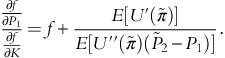
Differentiating the indirect utility function with respect to any parameter, α, yields:

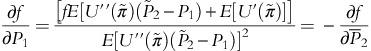
Setting α=P1, K and using the first order conditions implied by (3) leads to the following:


Equation (7) is a useful result as it provides for a way to estimate the optimal number of futures contracts as partials of the indirect expected utility function.Footnote 5 One route to empirical testing is to assume specific forms for the utility function and then to test if the assumed form is in conformity with the data. A more efficient method, however, is to approximate the form of the indirect utility function through a generalized Taylor series expansion and then impose empirical restrictions to test for specific forms.Footnote 6 This method is used below. Expanding the indirect utility function by a second order Taylor seriesFootnote 7 around an initial expansion point, Z, yields:

where V
i
are first partial derivatives of the indirect utility function equal to 


 V7=V
σ
,
V7=V
σ
,  V9=V
K
and V
ij
=V
ji
are second partial derivatives. All derivatives are evaluated at the expansion point Z with D
i
and D
j
representing deviations from the expansion point. Thus,
V9=V
K
and V
ij
=V
ji
are second partial derivatives. All derivatives are evaluated at the expansion point Z with D
i
and D
j
representing deviations from the expansion point. Thus, 
 and so on. Differentiating (8) with respect to P1 and K results in:

The first set of parameter restrictions imposable in (9) results from the equality of cross-partials. This yields the restriction V89=V98. Another source of refutable hypotheses are provided by the intrinsic features of the model as represented by the comparative statics of the model. Following Dalal (1994), however, it is easier to derive these results using the partials of the indirect utility function.Footnote 8 Now (4) and (5) imply that:

Young’s theorem then immediately implies that  (or V88=−V68=−V86) and
  (or V89=−V69=−V96). These results then imply that all the general parameter restrictions imposable in (9) are given by:Footnote 9

It is worth emphasizing that the restrictions given by (11) are implied by the intrinsic features of the model such as expected utility maximization and risk aversion. More stringent assumptions such as decreasing or CARA require additional restrictions on (9). These restrictions are derived and tested in the empirical section of the article.
DESCRIPTION OF THE DATA
Estimating (9) requires data on bank loans, deposits and equity as well as loan rates, deposit rates, borrowing rates, eurodollar futures prices and futures positions held by commercial banks. The data set involves monthly data from January 2001 to June 2007. Data on the derivatives activities of US commercial banks are provided by the OCC, which issues quarterly reports on bank derivative activities. It is apparent from these reports that derivatives activities are dominated by a very small group of large financial institutions. The data for the most recent quarter covered by the data set indicate that of the total notional amount of all derivatives contracts, an overwhelming 98 per cent is accounted for by five commercial banks (J.P. Morgan Chase, Citibank, Bank of America, HSBC and Wachovia) while 949 other commercial banks account for the remaining 2 per cent.Footnote 10 In terms of total assets, however, the top five banks account for only 48 per cent of all bank assets. Clearly, in studies of bank hedging it is more appropriate to focus on the few large banks that hedge rather than on all commercial banks. Previous research in this area (Doukas and Arshanapalli, 1992) that utilizes data for all commercial banks seems misplaced. Data on bank loans, deposits and equity for the top five banks that hedge are accordingly drawn from balance sheets in Call Reports published by the Federal Financial Institutions Examination Council (FFIEC).Footnote 11
Actual data on long/short futures positions are not contained in bank financial statements. Exhaustive financial information pertaining to derivatives is contained in Consolidated Reports of Condition and Income provided by the FFIEC. One of the schedules (Schedule RC-L: Derivatives and Off Balance Sheet Items) contain very detailed information on bank derivatives positions. However, this information is reported in gross notional amounts from which it is impossible to infer actual long/short positions.
Actual futures positions for US banks were obtained from BPR reports provided by the CFTC. The BPR data are derived from Schedule 1 of CFTC Form 40, which requires bank affiliated traders to certify if a trader is commercially engaged in business activities hedged by use of the futures or options markets. These data are used to generate the BPR data. I used that portion of the report that pertained specifically to futures hedging positions.
Among the interest rate futures contracts available to banks for hedging, the eurodollar futures contract is by far the most widely used contract. Since the 1981 launch of the eurodollar futures contract by the Chicago Mercantile Exchange (CME), the CME eurodollar futures contract has metamorphosed into the world’s most actively traded futures contract. The contract is based on a 3-month eurodollar time deposit equal to $1 million with expiry dates in March, June, September and December. The eurodollar contract is by far the preferred futures instrument for bank hedging. The open interest held by banks in this contract is roughly 4.50 times the open interest in the next most widely held interest rate futures contract – the Chicago Board of Trade’s 10 year US Treasury Note. Bank participation accounts for roughly about 10 per cent of the total activity in the eurodollar futures market.
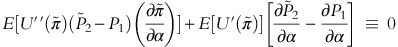
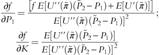
Eurodollar futures prices for the contract closest to expiration (that is, nearby contract) were obtained from the Commodity Research Bureau. The futures price used in the data set corresponds to the exact date every month on which the CFTC releases data on bank futures positions. Data on loan rates, deposit rates and borrowing rates are widely available. The loan rate was modeled as the prime loan rate, the deposit rate as the 3-month certificate of deposite (CD) rate and the borrowing rate as the fed funds rate. Summary statistics on the data that span monthly data from January 2001 to June 2007Footnote 12 is reported in Table 1.
EMPIRICAL RESULTS
The final form of the estimation equation with all cross-equation and symmetry restrictions is given by:

The equation above is a non-linear estimation equation. The dependent variable in (12) is the optimal net futures position, which is determined by nine independent variables. Thus, the independent variable D1 is the mean quantity of bank loans  , which is expressed in the estimation equation as deviation from its mid-point value
  (or as
  D2 is the mean return on bank loans, D3 is mean return on borrowed funds, D4 is mean return on deposits, D5 is mean quantity of deposits, D6 is mean futures price at maturity of the futures position, D7 is standard deviation of the futures price, D8 is mean futures price at inception of the futures contract, D9 is fixed cost. All of these independent variables are expressed in deviation form. An intrinsic feature of the model here is that it explicitly incorporates risk aversion. In fact, the incorporation of risk aversion is the underlying reason for the non-linear nature of the model. Risk neutrality, for instance, would have resulted in a simple linear model. This is explicitly demonstrated below.
Equation (12) was estimated using a non-linear, least squares regression procedureFootnote 13 using monthly data over the period from January 2001 to June 2007. The estimated form of (12) is reported in Table 2.
An intrinsic feature of the model estimated above is that it explicitly incorporates risk aversion. A straightforward test of the validity of this assumption is to consider the alternative hypothesis of risk neutrality. Risk neutrality implies that  Since V
K
=−E[U′(π*)], risk neutrality implies that all partial derivatives of V
K
(=V9) given by V
Kθ
=−E[U″(π*)((∂π*)/(∂θ))]=0 where
Since V
K
=−E[U′(π*)], risk neutrality implies that all partial derivatives of V
K
(=V9) given by V
Kθ
=−E[U″(π*)((∂π*)/(∂θ))]=0 where  In addition, under risk neutrality, the firm is insensitive to the standard deviation of the futures price given by σ implying that
  Risk neutrality thus implies a simple, linear estimation form given by:

The difference in the forms of the estimating equations given by (12) and (13) clearly highlight the difference that risk aversion makes to the form of the estimating equations. Assuming risk aversion complicates empirical estimation by rendering the linear form implied by risk neutrality into the non-linear form implied by risk aversion. The estimation results of (13) are reported in Table 3.
The test statistic is given by −2(lnλ) where lnλ is the log of the likelihood functions of the restricted and unrestricted models. Under the null hypothesis, the test statistic is distributed as chi-square [χ2] with degrees of freedom equal to the number of independent restrictions. The calculated χ2 value is 47.84 while the critical χ2 value at the 5 percent level with nine independent restrictions is 16.92. Clearly, these restrictions are rejected implying that risk neutrality is not a valid description of the underlying data.
FORWARD UNBIASEDNESS, CARA AND THE MSS MODEL
The assumption that the forward rate is an unbiased predictor of the future spot rate is a common assumption in the empirical hedging literature. In addition to the unbiasedness of the forward rate, the assumption that the utility function exhibits CARA is commonly used to simplify the derivation of optimal futures positions. Both Koppenhaver (1985, 1990) and Morgan et al (1988) assume unbiasedness and CARA in deriving optimal futures position for financial institutions. The validity of these assumptions is, however, unclear. Consequently, this section tests the empirical validity of these assumptions.
Define the following variables: 

 (the spread between the loan rate and borrowing rate),
 (the spread between the deposit rate and borrowing rate),
  Equation (3) then implies that:

Using Rubinstein’s (1974) theorem (that is,  ), and noting that the coefficient of absolute risk aversion is given by
  the above can be rewritten as:

Solving for the optimal futures position, f* results in:

With forward unbiasedness,  Thus:
Thus:

where  is the slope coefficient from a linear regression of
  on
on  The other variables are defined similarly. Equation (14) then implies that the optimal forward position is a linear combination of regression coefficients from four separate regressions:
-
a)
a regression of the the deposit-borrowing spread on the futures price;
-
b)
a regression of the deposit rate on the futures price;
-
c)
a regression of the loan-borrowing spread on the futures price;
-
d)
a regression of the loan rate on the futures price.
For (14) to be valid at least two restrictive assumptions – CARA and martingale efficiency in the futures market – must holdFootnote 14 If either of these assumptions does not hold, the estimating form given by (14) cannot be used to estimate the optimal futures position. Equation (14) was estimated using quarterly data from January 2001 to June 2007. It was clear from an examination of the fitted values that the estimated futures positions bore little resemblance to actual positions implying that either the assumption of futures unbiasedness or CARA is incorrect. Of both these assumptions, CARA is the easier one to test. This is tested in the next section.
TESTING FOR CARA
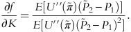
The most straightforward assumption about risk-averse behavior is to assume that financial institutions exhibit CARA. The utility function under CARA is given by  where A is the coefficient of CARA. The empirical restrictions implied by CARA are given by differentiating (6) with respect to P1 thus:

Since 
 the above results in

Utilizing (3) ands (5), the above implies that

Note that both  and A must be positive. At the point of approximation
  , which is positive for net long positions and negative for net short positions. In essence this means that under CARA,
  In addition, the comparative statics results imply that under CARA, the optimal amount hedged is invariant to fixed costFootnote 15 or (∂f*)/(∂K)=0. As
  CARA implies that:

With V K normalized to 1 at the expansion point, (17) results in:

Thus, V89≠0 requires that V99≠0. In addition to the restrictions given by the intrinsic features of the model as specified in (11), an empirical test for CARA can be formulated by imposing the following additional restriction:Footnote 16

For CARA to be valid, the restrictions given by (19) should not hold. The restrictions given by (19) were imposed on the unconstrained model given by (12) and are reported in Table 4.
The calculated χ2 statistic is equal to 1.34 and the critical χ2 value with two independent restrictions is 5.99. Clearly, the restrictions imposed on the empirical model estimated in Table 3 cannot be rejected, implying that CARA does not seem to be the underlying utility form.
BANK HEDGING IN FUTURES MARKETS
The results above imply that the models of bank hedging used in much of the previous literature, underpinned by assumptions such as CARA and forward unbiasedness, do not seem to have much empirical support. The logic underlying these assumptions is clear – without CARA and forward unbiasedness the derivation of the optimal hedge position becomes excessively complicated. This article, however, shows that the derivation of the optimal futures hedging position is not conditional on making any such simplifying assumption.
The rejection of CARA in the previous section implies that the underlying data are consistent with the form described by (12) and reported in Table 2. It should be noted that this form is derived under no restriction stronger than those implied by the intrinsic features of the model such as reciprocity and symmetry relationships. I turn now to an empirical analysis of this estimated form.
The parameters of the model are given by  To assess the empirical effects of a parametric change on the optimal hedging position (f*), differentiate (12) with respect to a given parameter. Suppose, for instance, that we are interested in assessing the effect of a change in
  (the rate on borrowed funds), on f*. Recalling that
  and differentiating (12) with respect to
  results in:

where δ and η are the denominator and numerator of (12). Evaluating the above at the expansion point where D
i
=0 implies that δ=1 and  Thus
Thus

Using the empirical estimates from Table 2 it can be easily determined that an increase in the expected borrowing rate leads to a change in the net futures position of banks equal to 266 623 short contracts (that is, V83−V93V8=442 180−(−4.48)(−158 215)=−266 623).Footnote 17 As interest rates rise, eurodollar futures prices fall leading to a profit on short eurodollar futures positions. The results thus imply that an expected increase in interest rates and the subsequent rise in funding cost is hedged by banks through increasing their short futures positions.Footnote 18 Similarly, the empirical results imply that an increase in the current futures price, P1, changes the net futures position by 136 145 contracts. Note that this effect is equal to and opposite to the effect of an increase in  (the expected futures price at maturity) – a result that is implied by the underlying theory (see equation (10)). The impact of changes in other parameters on the optimal hedging position can be similarly determined. These are reported in Table 5.
All estimated values in Table 5 are consistent with the range of values reported in the BPR on bank’s use of the eurodollar futures market. The most striking result is the fact that banks seem to respond to price changes while quantity changes seem to have virtually no influence on bank hedging. Note for instance that changes in both loan and deposit quantities seem to have no effect on the hedge position. Similarly, the amount of equity capital (which is treated as a proxy for fixed cost) has no effect on the hedge position. The reason for this may be because of the underlying rationale of futures hedging itself. Futures hedging is effective as a method of managing short-run deviations in profits – in effect, a first order risk management response. Thus, while changes in short-term rates can be effectively managed in the futures market, it is far less likely that longer-term systemic trends represented by changes in quantities and equity capital can be managed through futures hedging. In the literature, the role of equity capital in the determination of the optimal futures positions has often been ignored. The empirical results here lend support to that approach.
CONCLUSION
McDonald (2006) points out that we know surprisingly little about the manner in which financial institutions hedge risk. Part of the problem is that accounting statements provide very little transparency about the actual hedging positions assumed by financial institutions. Compounding this is the fact that futures positions reported by organizations like the CME are rarely broken down by type of institution.
In this article, data from the OCC are used to identify a set of financial institutions, which account for a substantial majority of interest rate derivatives positions. This information is used along with data on Bank Participation Reports provided by the CFTC to examine specific characteristics of futures hedging by financial firms at a level of detail that has not so far been reported in the literature. I identify the types of quantity and rate risks hedged by banks, the sensitivity of observed futures hedging positions to changes in market variables and the impact of risk aversion on hedging behavior.
The results here indicate that while bank futures hedging positions are insensitive to quantity risks they are far more sensitive to rate changes. The results here also indicate that commonly used simplifying assumptions in the literature (CARA, forward market unbiasedness) are not supported by actual hedging data.
Notes
See Survey of Terms of Business Lending, 13 December 2007 published by the Federal Reserve Bank.
A market quote of 95 implies that the 90-day eurodollar interest rate underlying the contract is 5 per cent p.a. or 1.25 per cent per quarter. For a $100 ($1 million) par value this implies a contract price of 98.75 ($987 500).
The second order conditions are given by:
 which is negative with risk aversion.
Equation (7) can also be derived using standard comparative statics. Differentiate (3) with respect to any parameter. Thus:
Setting this equal to P1 and K results in:
Multiplying the top and bottom by
 and using (3) implies the result in (7).
This method has been used in empirical work by Park and Antonovitz (1992); Doukas and Arshanapalli (1992); Dalal and Arshanapalli (1993); and Satyanarayan (1999).
See Hlawitschka (1994) for a discussion of the empirical nature of Taylor series approximations to expected utility. Hlawitschka presents empirical evidence that second order Taylor expansions provide excellent approximations to expected utility even when the series does not converge.
Empirical work on uncertainty is fairly sparse. However, even extant empirical work is marred by errors possibly because of the complexity involved in empirical modeling under uncertainty. See an excellent paper by Dalal (1994) who comments on methodological errors in the empirical uncertainty literature). An otherwise interesting paper by Doukas and Arshanapalli (1992), which uses similar techniques to this article, is marred by several methodological issues. Doukas and Arshanapalli differentiate the indirect utility function with respect to random variables. The correct procedure, however, requires specifying the nature of the distribution of the random variable and then differentiating with respect to the non-stochastic parameters of the distribution (Silberberg, 1990, p. 457). In deriving the empirical restrictions, an additional restriction
 using Doukas and Arshanapalli’s notation, is implied but not imposed on their model (see equation 12, p. 181).
These results can also be shown using standard methods. The comparative statics results of the model imply that:
and by Young’s theorem:
Other reciprocity relations can be derived but these are not imposable in (9).
The percentage held by the top five banks for interest rate derivative contracts (as opposed to all derivatives contracts) is similar.
Loans are defined as loans/leases held for sale plus loans/leases net of unearned income (items 4a+4d in the Call Reports). Deposits are defined as domestic and foreign interest bearing deposits (items 13a2+13 b2). Equity is total equity capital (item 28), which is used as an estimate of K.
Data on loans, deposits and equity are obtained from the balance sheet of banks as reported in the bank Call Reports. These data are, however, provided only every quarter. This quarterly series was extrapolated into a monthly series using a simple weighting procedure. Given a quarterly figure on loans for say, December and March, the loan figure for January was calculated as a weighted average of the data for December and March using weights of 2/3 and 1/3, respectively.
It should be noted that (12) is derived from a Taylor series approximation and thus holds exactly only at the point of expansion. At the expansion point, which is the set of values corresponding to the midpoint of the data set, D i =0. For estimation purposes V9 is normalized to 1 implying that at the point of estimation, f*=V8.
In fact, (14) can be further simplified by assuming that deposits are non-random. (Koppenhaver (1985) makes this assumption in part of his paper). With non-random deposits the optimal futures position reduces to:
 where
where 
 is the slope coefficient from a linear regression of
  on
on 
The comparative statics results imply that:
 With CARA,
 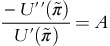 or
or  Multiplying both sides of the above equality by
  and utilizing the first order conditions implies that (∂f)/(∂K)=0.
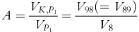
If the ressstrictions given by (19) are rejected, the hypothesis of CARA cannot be rejected. In that case, using (5) and (16) an empirical estimate of the coefficient of risk aversion, A, is given by:
The point at which these derivatives are assessed is the mid-point of the data set corresponding to June 2004. During this month, the futures position of banks in the eurodollar futures markets was 524 609 long contracts and 533 249 short contracts or a net short futures position equal to −8640 contracts. Strictly speaking, therefore, the total change is equal to a change of 275 263 short contracts.
During the period considered in this article (June 2001 – June 2007), the minimum and maximum number of eurodollar futures contracts traded by banks for hedging purposes varied between 221 000 contracts to 1.50 million contracts per month. The maximum net short position during this period exceeded a million contracts. The estimates reported in Table 5 are therefore representative of actual positions in the market.
 which is negative with risk aversion.


 and using (3) implies the result in (7).
 using Doukas and Arshanapalli’s notation, is implied but not imposed on their model (see

 where
where 
 is the slope coefficient from a linear regression of
  on
on 
 With CARA,
  or
or  Multiplying both sides of the above equality by
  and utilizing the first order conditions implies that (∂f)/(∂K)=0.
References
Basel Committee on Banking Supervision. (1993) Measurement of Banks’ Exposure to Interest Rate Risk. Switzerland: Basel.
Basel Committee on Banking Supervision. (2004) Principles for the Management and Supervision of Interest Rate Risk. Switzerland: Basel.
Dalal, A. and Arshanapalli, A. (1993) Estimating the Demand for Risky Assets via the Indirect Expected Utility Function. Journal of Risk & Uncertainty 6 (3): 277–288.
Dalal, A. (1994) Econometric tests of firm decision making under uncertainty: Optimal output and hedging decisions: Comment. Southern Economic Journal 61 (1): 213–217.
DeMarzo, P.M. and Duffie, D. (1991) Corporate financial hedging with proprietary information. Journal of Economic Theory 53 (2): 261–286.
Diamond, D.W. (1984) Financial intermediation and delegated monitoring. Review of Economic Studies 51 (3): 393–414.
Doukas, J. and Arshanapalli, A. (1992) Interest rate risk management with futures for intermediaries. Applied Financial Economics 2 (3): 179–185.
Flannery, M.J. and James, C.M. (1984) The effect of interest rate changes on the common stock returns of financial institutions. Journal of Finance 39 (4): 1141–1153.
Hlawitschka, W. (1994) The empirical nature of Taylor-series approximations to expected utility. American Economic Review 84 (3): 713–719.
Ho, T. and Saunders, A. (1983) Fixed rate loan commitments, take down risk, and the dynamics of hedging with futures. Journal of Financial and Quantitative Analysis 18 (4): 499–516.
Koppenhaver, G.D. (1985) Bank funding risks, risk aversion, and the choice of futures markets. Journal of Finance 40 (1): 241–255.
Koppenhaver, G.D. (1990) An empirical analysis of bank hedging in futures markets. Journal of Futures Markets 10 (1): 1–12.
Leland, H.E. (1998) Agency costs, risk management, and capital structure. Journal of Finance 53 (4): 1213–1243.
McDonald, R. (2006) Derivatives Markets. Boston, MA: Addison-Wesley.
Morgan, G. and Smith, S. (1986) Basis risk, partial take down, and hedging by financial intermediaries. Journal of Banking and Finance 10 (4): 467–490.
Morgan, G., Shome, D. and Smith, S. (1988) Optimal futures positions for large banking firms. Journal of Finance 43 (1): 175–195.
Park, T. and Antonovitz, F. (1992) Econometric tests of firm decision making under uncertainty: Optimal output and hedging decisions. Southern Economic Journal 58 (3): 593–609.
Purnanandam, A. (2007) Interest rate derivatives at commercial banks: An empirical investigation. Journal of Monetary Economics 54 (6): 1769–1808.
Rubinstein, M. (1974) An aggregation theorem for securities markets. Journal of Financial Economics 1 (3): 225–244.
Satyanarayan, S. (1999) Econometric tests of firm decision making under dual sources of uncertainty. Journal of Economics & Business 51 (4): 315–325.
Schweser, C., Cole, J. and D’Antonio, L. (1980) Hedging opportunities in bank risk management programs. Journal of Commercial Bank Lending 62 (1): 29–42.
Sealey, W. (1981) Deposit rate setting, risk aversion, and the theory of depository financial intermediaries. Journal of Finance 35 (5): 1139–1154.
Silberberg, E. (1990) The Structure of Economics: A Mathematical Analysis. New York: McGraw-Hill.
Smith, C. and Stulz, R. (1985) The determinants of firm’s hedging policies. Journal of Financial and Quantitative Analysis 28 (4): 391–405.
Author information
Authors and Affiliations
Corresponding author
Rights and permissions
About this article

Cite this article
Raju, S. Risk aversion, bank funding risk and futures hedging. J Deriv Hedge Funds 20, 241–255 (2014). https://doi.org/10.1057/jdhf.2014.21
Received:
Revised:
Published:
Issue Date:
DOI: https://doi.org/10.1057/jdhf.2014.21