
Abstract
Wind turbine generators (WTG) is predicted to play a prominent role in the electric power systems of the future. Connection of wind turbine generators to the distribution network increases power sources and therefore increases reliability of distribution network. Assessment of reliability of distribution network connected to wind turbine generators based on two state model yields big errors due to dependence of wind source capacity on wind speed which is a variable value. For more accurate assessment results, the article proposes to utilize multi-stage model of wind source reliability and switch section partitioning based on reliability on distribution network.
1 Introduction
The distribution networks (DNs) are responsible for supplying electricity directly to the consumers. Therefore, they are responsible for ensuring the quality of electricity service. Changes in grid configuration, status parameters and equipment status in the DNs directly affect the consumers through changes in power quality and power supply reliability [1]. In terms of power quality, DNs is mainly determined by voltage quality indicator. The most effective voltage regulating components such as transformers, compensators are located in the DNs. In different modes of the load, the DN could modify the configuration to ensure the determined voltage quality. In relation to the power supply reliability, DN plays a crucial role because power outage in DN could directly affect the power shortage on the load. In order to improve the reliability in the DN, several measures could be implemented such as installation of reclosers, isolators, grid reconfiguration, etc.
As a sequence, indicators such as the system average interruption frequency index (SAIFI), customer average interruption frequency index (CAIFI), system average interruption duration index (SAIDI), customer average interruption duration index (CAIDI) are widely used to evaluate the power reliability. Determining the relationship between these indicators and the change in power supply is the first step in introducing the solutions to enhance the power reliability of DNs.
One of the highly accurate methods for power reliability assessment is section partitioning. This method employs partinioning switch to partition the grid into secctions with different power reliabilities. It is assumed that failures of the fuses are neglectable, the durations of electricity service interupted to consumers in the same section are similar. Then, configuration by sections shall be basis for analyzing and calculating the power reliability to consumers. In one DN, it is possible to partition it into several load sections. These load sections could be patitioned by interconnected lines by non-automatic breakers devices such as cut-out fuses, disconnecting switch, load switch which are characterized by the same failure’s causes and frequency [2]. The accuracy of calculating the power reliability depends on the reliability model of the elements in the DN. Normally the elements are modeled under two states of success and failure associated with two parameters of failure probability and resilience probability. With this model, higher errors may be expected as when modeling with multi-state generators such as Wind Turbine Generator (WTG). Recently, wind power integration to the DN has been increased to improve the power supply capability and reduce the probability of power shortage due to lack of power supply.
However, WTG is characterized by unmanageable output power which is entirely dependent on the wind speed as random variable. Thus, this article proposes to utilize multi-state model of wind source reliability and switch section partitioning based on reliability on distribution network to achieve more accurate results of calculating the yearly duration of power shortage due to failures.
2 Reliability Model
2.1 Reliability Model of Multi-state WTG
2.1.1 Wind Velocity Model
Wind speed varies by locations and time. A common expression of wind velocity randomness is the probability density function model Weibull [3].
In which:
ν is wind velocity (m/s); k is the character index varies with the wind of each region (Fig. 1); c is the rate index calculated based on the average annual wind speed, calculated over several years, shown in Fig. 2.

Probability distribution function with different k values

Probability distribution function with different c values
Probability distribution function:
In this paper, the distribution of wind speed probabilities is described based on the annual average value µ and standard deviation σ [3]. With deviation range 10σ, the distribution will include very low probability values. The distribution is divided into Nb steps at scale of 10σ/Nb. Step center value SWbi (i = 1,…, Nb) is defined in Eq. (3) corresponding to the probability of each step Pbi (i = 1,…, Nb) is defined in the Eq. (4).
where Nbi is the number of wind speed data simulation; Ny is the number of years of simulation (Fig. 3).

Simulation of wind speed by mean value in μ and standard deviation σ [3]
2.1.2 Generating Capacity Model of WTG
Generating capacity of WTG directly depends on wind speed. Typical speed thresholds for each WTG:
- Vci:
-
minimum operational wind speed;
- Vr:
-
wind speed for starting the turbine reaching the rated power;
- Vco:
-
maximum wind speed allows turbines to operate (for reasons of safety for turbines when the wind is over speed) (Fig. 4).
Fig. 4 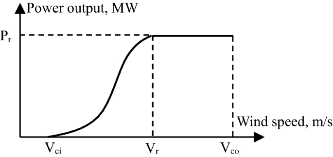
Characteristics of WTG output power at wind speed [4]

For each wind speed value is a generating output value:
Values of A, B, C are calculated in the following formulas [5]:
2.1.3 Multi-state Model of WTG
For WTG with the generating depends on the change in wind speed, the two-state model is unable to describe all generating states. Therefore, it is required to use a multi-state model in order to accurately depict the actual state of the WTG. Each state is characterized by the state power Pi and the state probability PBi shown in Fig. 5.

Status probability of generating capacity of WTG
The multiple state model presents many advantages that accurately describe the working status of the WTG changes according to wind speed. However, the model encountered many difficulties when calculating the probability of special states when number of states is high. Therefore, simplified multi-state model was proposed in [6] as in Fig. 6.

Simplified multi-state model
2.2 Computation of Reliability in Distribution Network
2.2.1 Distribution Network Section Partitioning
During the reliability calculations, complex grids are often partitioned into sections with the same reliability parameters. With the DN having large number of nodes, partitioning DN into sections is necessary so as to simplify reliability computation. Section partitioning by reliability is subject to location of the switch. If the failure of the fuse is assumed to be neglectable, the supply of electricity to consumers in the one section is the same. In fact, section partitioning based on automatic switches devices also help improving reliability. In case of failure, sections isolated from the main grid could be offgrid. Distributed generators feeding to these offgrid sections may become main supplier for those sections’ loads.
Determination of isolating location to ensure continuous power supply to the load depends on the correlation between the distributed generator capacity and the loads. For the pro-active generators such as diesel, small hydropower, it is possible to determine the power source. Whereas, determination of isolating location faces many difficulties with distributed generator which generating capacity depends randomly on the wind speed parameter.
The IEEE RBTS 25 node grid model on Fig. 7 [7] is partitioned into five sections with different reliability. In particular, in order to improve reliability of Sects. 2, 3, 4, 5, WTG was integrated. These sections can be isolated from the main grid to operate independently in case of failure through the island conditioning unit such as circuit breaker. In the absence of wind power, the cause of the power failure in each Area ith (KVi) can be a fault on the distribution station (DS) that located on the line connected to KVi from the main power supply or on KVi itself. For example, for KV3 on set G4 = {KV1, KV3, KV4, DS}. For every failure of each component of the set G, the power failure duration on KV4 is the duration of repair of the defective part [7].

Section partitioning of grid by reliability
Then, duration of the power outage is calculated as follows:
In which:
T NDk is the duration of off-grid for section k; λi is fail intensity of element i in element j; ri is duration of repairing of element i; and m is the number of elements in section i.
If every section is consider as smaller system within DNs, each section has SAIDIk and the whole system has SAIDIs. The two indexes are associated through the formula (9):
In which:
Ck is the number of load in section k; Cs: total number of loads in the whole DN.
In fact, duration of power shortage is different with formula (13), because sections have distributed generator and operating off-grid. Thus, it is necessary to include the probability function of off-grid mode as follows:
2.3 Calculating Power Reliability of Distribution Network
In section a, the probability of operation in off-grid mode has been discussed. However, the success of grid isolation is subject to co-relation between capacity of distributed generators and load capacity at the time of isolation. To calculate the reliability indices, it is necessary to calculate the probability of power shortage, when power shortages occur:
In which:
SWTG, capacity of wind power integrated to the section in off-grid mode; SL: load capacity at the time of grid isolation; τi, is the time of SWTG < SL, is determined based on extended load curve of the section and capacity Pi at the state i.
From the formula (10) and (11), probability of power shortage when isolating from the grid for the section in consideration:
Sectional reliability is determined:
Once sectional reliability is determined, system reliability can be identified by formula (9).
3 Case Study
3.1 Network Configuration
See Table 1 here.
3.2 Wind Power Source
One WTG with parameter given in Table 2.
3.3 Absence of WTG
Based on set in Tables 1, 2, 3, 4, 5, SAIDI index was determined for sections and for system in the absence of WTG. Results are shown in Table 6 (Fig. 8).

Extended load curve of KV4 (on the left) and KV5 (on the right)
3.4 Considering Integrating WTG
Considering integrating WTG in Table 2 into DN. Calculating SAIDI4, off-grid probability:
In off-grid mode, power shortage may occur when WTG is unable to meet the demand. Power shortage probability is detemined based on time of power shortage expressed in load curve in different states of wind power (Table 7 and Figs. 9, 10). The same process was applied for other sections, the results are shown in Table 8.

The relationship between wind turbine capacity and capacity shortage

The relationship between Power probability and shorage probability
The calculation results in Table 8 and Fig. 11 indicate that:

SAIDI index for each section (with and without WTG integrated)
-
The average System Average Interruption Duration of DN with WTG integrated is substantially improved compared to the case of DN without WTG integrated, especially in sections directly connected to the WTG.
-
The similar results are also found in the offgrid mode, when the WTG capacity increases, the probability of power loss and power loss time decreases. When capacity of wind power is significant enough compared to total load capacity in the DN, the power supply reliability has been significantly improved.
-
Section partitioning contributes to improve accuracy of power reliability assessment. The power reliability model of multi-state WTG facilitate the consideration of randomness of wind power and load characteristics explicitly.
4 Conclusion
Determining the power reliability of DN integrating wind power is a complex problem. When considering this, it is necessary to take into account influencing factors, especially DN configurations, randomness of wind speed affecting WTG generating capacity and load characteristics. For wind power, the traditional reliability model is no longer suitable because it is unable to stimulate states of WTG.
The multi-state model should be used for this purpose. This study has employed a multi-state model of wind power to calculate several reliability indexes considering the characteristics of the sectional load. In this paper, we have not considered in the case of DN integrated by multiple distributed power sources with different generating capacity characteristics. However, it is probable that the proposed method is capable to investigate such problems.
References
von Meier A (2006) Electric Power systems: a conceptual introduction. Wiley-IEEE Press, Hoboken
Duc Hanh N (2011) Invetigation on improvement of economic efficiency, voltage quality and reliability in the planning of medium voltage electrical network, Doctoral thesis; Hanoi (in Vietnamese)
Boyle G (2004) Renewable energy. Oxford University Press, Oxford
Wu L, Park J, Choi J, EI-Keib AA (2009) Probabilistic reliability evaluation of power systems including wind turbine generators considering wind speed correlation. J Electr Eng Technol. https://doi.org/10.5370/JEET.2009.4.4.485
Cheng H, Hou Y, Wu F (2014) Probabilistic wind power generation model: derivation and applications. Int J Energy 5(2):17–26
Ding Y, Cheng L, Zhang Y, Xue Y (2014) Operational reliability evaluation of restructured power systems with wind power penetration utilizing reliability network equivalent and time-sequential simulation approaches. J Modern Power Syst Clean Energy 2(4):329–340
Atwa YM, El-Saadany EF (2009) Reliability evaluation for distribution system with renewable distributed generation during islanded mode of operation. IEEE Trans Power Syst 24:2
Acknowledgements
This paper is developed as a subsidiary component of the study “Research on methodology and software to assess the power system reliability with consideration of renewable energy and other fuels for Vietnam power plants” Code: VAST.07.04/16-17. The authors specially thank the Vietnam Academy of Science and Technology—Institute of Energy Science for providing fund and creating favor in data collection during the implementation of the study.
Author information
Authors and Affiliations
Corresponding author
Additional information
Publisher's Note
Springer Nature remains neutral with regard to jurisdictional claims in published maps and institutional affiliations.
Rights and permissions
Open Access This article is distributed under the terms of the Creative Commons Attribution 4.0 International License (http://creativecommons.org/licenses/by/4.0/), which permits unrestricted use, distribution, and reproduction in any medium, provided you give appropriate credit to the original author(s) and the source, provide a link to the Creative Commons license, and indicate if changes were made.
About this article

Cite this article
Chuong, T.T., Van Hung, N. & Nam, N.H. Assessment of Wind Turbine Generators on Reliability of Distribution Network. J. Electr. Eng. Technol. 14, 2217–2224 (2019). https://doi.org/10.1007/s42835-019-00244-4
Received:
Revised:
Accepted:
Published:
Issue Date:
DOI: https://doi.org/10.1007/s42835-019-00244-4