Novel semantic tagging detection algorithms based non-negative matrix factorization

Abstract

The tagging aims to address a challenge to search relevant text-documents given a set of tags. In addition, the tag-based approaches received a wide attention as a possible solution to the big-content. Probabilistic topic model methods, such as Dirichlet distribution and non-negative matrix factorization are used for tagging process. Both have many challenges. The iterations in addition the semantic coherence are considered as challenges in semantic tagging applications. In light of this, we propose a novel learning tagging model called semantic non-negative matrix factorization, which introduces the utilization of the semantic text representation via knowledge-based approach to extract the term-topic matrix and the topic-document matrix by semantically approach. The proposed words are based on a novel initialization method for non-negative matrix factorization technique. In the experimental evaluations, we use five datasets demonstrate the effectiveness of our model. The results are compared with the state-of-the-art model. The results show the proposed model has an ability to generate more precise topics with semantically related and having the high sense to the disambiguation of meaning, provides up to more dimensionality reduction and the topic coherence based semantic.

1 Introduction

With increasing the amount of the data and the emergence of the big data, the processing and the analyzing requires the different technology from the earlier. The content management system, such as Wikipedia stores and links the huge number of documents and files. There is a lack of semantic linking and analysis. To reduce the number of references for a selected content, there is a need for semantic matching [1]. Tags (categories, or topic) are set of terms serving as a bridge of communication between the user and the documents. Generally speaking, there are two groups of topic models, i.e., generative probabilistic models, such as latent semantic analysis (LSA), probabilistic LSA, and latent Dirichlet allocation (LDA), and non-negative matrix factorization (NMF) to generate the topic model for tag-based [2]. The word sense disambiguation (WSD) consists of assigning the proper meaning to a word in a certain context. Many pieces of research use the WSD with the topic model instead of word for semantic relation to improve the information extraction [3, 4]. Traditionally, LDA received much attention in the field of tag-based because of its extensible nature of the model design as a generative process [5]. The Dirichlet appropriation has no persuading semantic inspirations and clashes with two common suppositions of sparsity: (1) the majority of the subjects have zero likelihood in a report, and (2) the majority of the words have zero likelihood in a point. At long last, The Bayesian deduction confuses the blend of numerous necessities into a solitary multi-target theme model [6]. In the more, the probabilistic topic model tends to have stochastic elements in their initialization, which can lead to their output being unstable. In light that, the others propose a new ensemble topic modeling method based on non-negative matrix factorization (NMF), which combines a collection of unstable topic models to produce a definitive output [7]. The standard formulations of NMF algorithms include stochastic elements in their initialization phase, this random component can affect the final composition of the topics found, and the rankings of the terms that describe those topics, this called instability problem. NMF based the singular value decomposition (SVD) approximation of the document-term matrix can also provide a clear improvement over standard NMF methods [8]. In light of the semantic tagging, the tagging modelling (topic modelling) needs reduction technique based semantic [9]. Dimensionality Reduction (DR) can be done in 2 ways: the feature reduction and the feature selection [10]. In addition, the above methods may generate the topics incoherent semantically. because they lack the semantic text representation.

To tackle these problems, we propose a topic modelling via a lexical semantic approach in addition a novel non-negative matrix factorization method (SNNMF), which is outlined in Fig. 1. In this figure, the documents, synset and topic are denoted as Di, wi, Ti, respectively. The proposed SNNMF model can capture the semantics from the text corpus based on WSD in addition the lexical semantic similarity. In other words, our objective function combines the advantages of both the novel NMF model for topic modeling and the lexical semantic similarity for generating topics semantic coherent . In the Fig. 1, V, H, and W are the vector representations of documents, term-topic, and topic-document in the latent space. Each column of H is a topic. To achieve better interpretability, we use a multi-level of a dimensional reduction algorithm to solve the semantic coherence optimization. The proposed models are compared with the other state-of-the art method on five real-world text datasets. The quantitative experiments show the superiority of our models over other existing method in terms of topic coherence. The stability of SNNMF are cleared in a novel initialization method for NMF. Finally, we design an experiment to investigate the interpretability of the SNNMF model. By visualizing the top five terms of top one topics and analyzing their networks, we demonstrate that the topics discovered by SNNMF are meaningful and their representative terms are more semantically correlated. Hence, the proposed SNNMF is an effective topic model for texts.

Fig. 1

The overview of the proposed SNNMF model for learning topics from the text corpus, which is represented by lexical semantic correlations

The contributions of this paper are fourfold as the following:

• 1. Motivated by confectioning the semantic coherence of the generated topics, we propose an answer by adding the semantic learning to the representation of the generated topics (“Algorithm 1”).

• 2. Propose a novel learning mechanism to perform a dimensionality reduction for the selected features of the generated topics based on the semantic learning (Algorithms 2, 3 and 4).

• 3. Presenting a novel initialization method for NMF to reduce the iteration process, improve clusters (tags) by decreasing terms overlap between clusters and overcoming the insatiability result (Algorithm 5).

• 4. Reduce the multi-label classification problem (Algorithms 4 and 5).

The elaboration of this paper is organized as follows. In Sect. 2: some recent related work is briefly reviewed, Sect. 3: proposed solution (Methodology), Sect. 4: result, Sect. 5: conclusion and future work, at last in reference section.

2 Related work

In recent years, to satisfy the topic detection model results, some scholars have made attempts merge between the semantics approach (semantic text representation) with the core techniques of topic detection (tagging). This section briefly discusses on the related works from latent topic decomposition in addition to the semantic text representation.

2.1 Semantic text representation

For textual documents, the most traditional data representation strategy is based on the simple term occurrence information encoded by TF-IDF score. The question is how to interpret text documents instead of word occurrence in the document through explicit or implicit semantics. While this approach is by far the most used, useful information such as context is missing [11]. One simple strategy to overcome that is semantic text representation. The semantic text representation aims to represent the text documents by explicit readable keywords or terms, which can semantically describe the main topic of the given text documents. Out of several approaches in this direction, the WordNet has been utilized for semantically enhance the text representation for various applications [12]. Another approach in [13, 14] called distributional semantics (semantic space). In other words, semantics word embeddings. Word2vec and Glove are the two most popular semantic embeddings having the capability to capture the semantics of the language. In [15, 16] the authors proved that the performance of Word2Vec to detect semantic words relations decreases when the corpus size is reduced, this because the word2vec is built on the basis of the co-occurrence frequency of lexical units in a collection of documents. Semantic networks (e.g., WordNet) and semantic spaces have been two prominent approaches to represent lexical semantics. In contrast, WordNet is constructed on the basis of systematic lexical intuitions handled by human experts; the information encoded in small world of words is evoked from laypersons. WSD is a bottleneck in a semantic text representation. WSD is conventionally regarded as the task of identifying which of a word’s meanings (senses) is intended, given an observed use of the word and an enumerated list of its possible senses. In other words, WSD is the task to determine the word sense according to its context [17]. Solutions to WSD are mostly categorized into supervised and knowledge-based approaches. Many existing WSD studies have been using an external knowledge-based unsupervised approach because it has fewer word set constraints than supervised approaches requiring training data [18]. WSD: Knowledge-based methods rely on lexical databases such as WordNet as primary resources and use algorithms such as lexical similarity measures (Lesk) [19]. That’s what we used for our text representation in SNNMF.

In addition, we now turn our attention in semantic similarity and relatedness measurements, similarity is a special case of relatedness. Semantic relatedness is calculated with usage of vector space model, and some sort of similarity metric which is tending to be used with that, such as cosine similarity, or similar. It is measuring tendency of usage words together in sentences (or paragraphs, documents). In contrast, semantic similarity (sometimes called topological similarity), where similarity is measured by distance between terms by using ontologies. Ontology is directed acyclic graph containing definition of relationships between terms. One example of such an ontology is WordNet dictionary. Similarity measure with usage of ontology is length of shortest path between two terms. In addition to the path and depth-based measures, the information content (IC)-based measures in which the hyponymy subgraph in the taxonomy is used to determine how much information is carried by the concept such as Resnik [20]. In summary, the semantic text representation plays the main role to extract the latent topics having semantic coherence in addition to the semantic similarity between terms that is used in the topics modelling. The semantic text representation based WSD by LESK in addition to Resnik semantic similarity is considered in our topic modelling.

2.2 Latent topic decomposition

We now turn our attention to algorithms that aim at uncovering abstract topics from data. We start with the probabilistic models. In [21] the authors conducted a comprehensive review of various short text topic modeling techniques. This survey is based three categories of methods, first is based on Dirichlet multinomial mixture, second is based on global word co-occurrences, and the last is based on self-aggregation. Finally, they evaluate these state-of-the-art methods on many real-world datasets and compare their performance against one another and versus long text topic modeling algorithm. This work did not point out to any semantic representation for datasets. In [22] the authors presented a probability topic model called (TKM) based on automatically identifying characteristic keywords for topics for working on regular text. TKM hypothesis, a keyword score depends on how common the word is within the topic and how common it is within other topics. This model assumes that topics of a word in a sequence of words are heavily influenced by words in the same sequence. Therefore, words near a word with high keyword score might be assigned to the topic of that word, even if they on their own are unlikely for the topic. In [23] the authors presented a probabilistic topic model called MetaLDA for working on both regular and short texts, which is able to leverage the document, or word meta-information, or both of them jointly, in the generative process. The authors hypothesized, incorporating such meta-information directly into the generative process of topic models can improve modelling accuracy and topic quality, especially in the case where the word-occurrence information in the training data is insufficient. In [24] the authors developed a correlated tag learning (CTL) model for the semi-structured corpora based on the topic model to enable the construction of the correlation graph among tags via a logistic normal participation process. In [25] the authors proposed a probabilistic topic model that incorporates DBpedia knowledge into the topic model for tagging web pages and online documents with topics discovered. The model learns the probability distribution of each category over the words using the statistical topic models considering the prior knowledge from Wikipedia about the words, and their associated probabilities in various categories [25]. In [26] the authors proposed Wikipedia-category-concept mention latent Dirichlet allocation (WCM-LDA), which not only models the relationship between words and topics, but also utilizes the concept and category knowledge of entities to model the semantic relation of entities and topics. In [27] the authors deal with a probabilistic topic model through a technique called tag-weighted topic model (TWTM). TWTM was a framework that leverages the tags in each document to infer the topic components for the documents. In [28] the authors introduced Topic Grouper as a complementary approach in the field of probabilistic topic modeling. The algorithm starts with one-word topics and joins two topics at every step. It therefore generates a solution for every desired number of topics ranging between the size of the training vocabulary and one. The process represents an agglomerative clustering that corresponds to a binary tree of topics.

We now consider the non-probabilistic topic modelling, comprising strategies such as matrix factorization since it produces top-notch state-of-the-art performance without the limitations of probabilistic approaches, such as lack of observations when applied to short texts. In this case, a dataset with n documents and m different terms is encoded as a design matrix A ∈ R^n×m and the goal are to decompose A into sub-matrices that preserve some desired property or constraint. Our proposed framework is specifically tailored [29]. For non-probabilistic strategies. A well-known matrix factorization applicable to topic modelling is the non-negative matrix factorization (NMF) [30]. Under this strategy, the design matrix V is decomposed into two sub-matrices H ∈ R^n×k and W ∈ R^k×m, such that V ≈ Wx H^T . In this notation, k denotes the number of latent factors (i.e., topics), W is a relationship between documents and topics, and H encodes the relationship between terms and topics. The restriction enforced by NMF is that all three matrices do not have any negative element. When dealing with properly represented textual data, the design matrix usually contains non-negative term scores, such as TF-IDF, with well-defined semantics (e.g., term frequency and rarity). It is natural to expect the extracted factors to be non-negative so that such semantics can be somehow preserved. We thus consider NMF as our matrix factorization strategy of choice. As a final note, as with the probabilistic strategies, the non-probabilistic ones can also generate incoherent topics, which is not desirable. We shall revisit this matter in next section. Recent works have been proposed to improve the construction of topics by means of using semantic approach such as word embedding as auxiliary information for probabilistic topic modelling. In [31] the authors proposed a semantics-assisted non-negative matrix factorization (SeaNMF) model to explore short text topics. The method incorporates semantic correlations of the word-context into the model. The semantic correlations between the words and their contexts are learned from the corpus ‘ skip-gram view, which has been shown to be effective in revealing semantic relations between words. We consider SeaNMF as a baseline. there is no work that combines the lexical semantic word and non-probabilistic models. The main reason for the absence of works like ours is that the introduction of the richer information provided by the lexical semantics representation hampers the topics representation due to the lack of direct correspondence between topics and smaller semantic units (e.g., words) in these richer representations. Moreover, the lack of words in lexical may yield to loss more important information which makes the topic model is useless. As we shall see, we propose a new topic extraction strategy to mitigate these problems. In [32] the authors proposed a novel model called ‘‘knowledge-guided non-negative matrix factorization for better short text topic mining’’ (abbreviated as KGNMF), KGNMF integrated the word–word semantic graph regularization which can be learned from external knowledge base e.g., Wikipedia into the basic NMF for improvement in short text topic learning. In [33] the authors developed a general non-probabilistic topic modeling framework. The model included: (1) the introduction of new semantically-enhanced data representations for topic modeling based on pooling, and (2) the proposal of a novel topic extraction strategy-ASToC—that solves the difficulty in representing topics in its semantically-enhanced information space. ASToC used bag of word (BOW), information gain (IG), non-negative matrix factorization (NMF), Fesher vector (FV) To summarize, the authors instantiated five viable combinations: (1) BoW + NMF; (2) BoW + NMF + IG; (3) BoW + NMF + ASToC; (4) FV + NMF + IG; and (5) FV + NMF + ASToC . In [34] the authors proposed a semantic tag recommendation technique exploiting associated words that are semantically similar or related to each other using the inter-wiki links of Wikipedia. The candidate words were then rearranged according to importance by applying a link-based ranking algorithm and then the top-k words were defined as the associated words for the article. In [35] the authors introduced strategy called CluWords for topic modeling. CluWord included (1) the data representation for topic modeling based on syntactic and semantic relationships derived from distances calculated within a pre-trained word embedding space and (2) the proposal of a new TF-IDF-based strategy.

2.3 Summary

Table 1 represents the outline of the work done by various authors. We looked at among authors in two highlights. We saw these highlights ought to be incorporated into semantic topic model. Afterward, our model will incorporate these two highlights.

Table 1 Summary of work done by different authors for semantic of topic models

3 Proposed model (SNNMF)

In this section, we will first provide some preliminaries NMF for topic modeling. Then, we will propose our SNNMF model including the semantic algorithms to estimate latent representations of terms and documents.

3.1 Notations

The frequently used notations in this section are summarized in Table 2.

Table 2 Math notations used in this paper

3.2 Preliminaries

3.2.1 Topic detection via NMF

The NMF method has been successfully applied to topic modeling, due to its superior performance in clustering high-dimensional data. In vector space model, a corpus is represented by an m × n matrix V, where n is the vocabulary size, and m is the number of documents. A common assumption of topic modeling is that a latent topic can be represented as a distribution over the term. Then, a topic is a vector h in Rⁿ, and an n × k term-topic matrix H can be obtained by vertically combining k topics. With W, a document can be seen as a distribution over the k topics, which can be represented as a k × m vector w. It is common to use WH^T to approximate the document matrix. W is the document topic matrix, where each column has the topic distribution of a document. Good H and W could ensure that the difference between WH^T and the original document matrix V is small. SNNMF replace ≈ with = in Eq. (1). Suppose the current m × n document matrix is V, then NMF methods detect topics as follows: Given a topic number k, it tries to find an n × k term-topic matrix H and a k × m topic-document matrix W, which satisfy the following. Table 2 gives a summary of math notations and explanations.

$${\text{V}} \approx {\text{WH}}^{\text{T}}$$

(1)

Equation (1) is designed for the non-negative matrix factorization (NMF). Where V is the document-term matrix. It considers the term frequency inverse document frequency (tf-idf) matrix, W is the topic-document matrix and H is the term-topic matrix.

3.2.2 Problem statement

Due to the semantic text representation approach specially WSD in addition the semantic similarity, the conventional topic models are not effectively to capture semantic topics, which leads to the poor performance in semantic topic learning. To tackle this problem, we introduce semantic topic modelling SNNMF.

3.3 SNNMF overview

In this segment, we propose a novel semantic topic detection model (SNNMF). SNNMF is performed by a novel methodology for playing with a non-negative matrix factorization (NMF) with a semantic text representation approach. The strategy is intended for transforming the traditional BOW representation of documents to include semantic information related to the terms present in the documents. The semantic context is obtained by lexical semantic (WordNet). Our approach consists in transforming each document in a new representation where original words are replaced by a cluster of synset terms that we refer to as synsets. The transformation process is composed of two phases. In the first one, we compute, the WSD by algorithm (LESK) for each word of the dataset to obtain the sense term (synset). In the second phase, we compute a traditional version of the TF-IDF weighting scheme for the new features (synset), so that we can exploit these new terms as a richer representation of documents of the collection. These phases of our approach are described in preprocessing Sect. 3.4.1. Then, performing SNNMF algorithms from 1 to 5 that express that a novel initialization of NMF to obtain the term-topic matrix H and topic-document matrix W.

The advantages of detecting topics by SNNMF model come from four-fold. First, it is adding the semantic text representation to the representation of topics (such as semantic similarity based information content and WSD “Algorithm 1”). Second, it can reduce the overlaps between different topics based semantics (dimensionality reduction) and lead to more separable topics (Algorithms 2, 3 and 4). Third, it can reduce the iteration to achieve the stability to generate the term-topic and the topic-document matrix (Algorithms 4 and 5). fourth, based the second, it can reduce multi-label classification problem (Algorithms 4 and 5).

3.4 SNNMF details

This section discusses the details of SNNMF. SNNMF has three matrices (1) document-term, (2) term-topic, and (3) topic-document. SNNMF performs the document-term matrix (V ∈ R^m×n) by extracting synset terms using Eq. (3) from given text dataset . the document-term matrix(V) is considered in preprocessing step for term-topic matrix. SNNMF performs the term-topic matrix (H ∈ R^n×k) by two steps, first, the preprocessing and second, the dimensionality reduction. SNNMF performs the topic-document matrix (W ∈ R^k×n) after getting the V and the H. later, we will see in SNNMF W = V(H^t)⁻¹. SNNMF pipeline (Fig. 2) shows the flow of the proposed model (SNNMF) component sequentially.

Fig. 2

SNNMF pipeline

3.4.1 Prepossessing

In this section, the purpose of this step is obtaining a first term-topic matrix (H⁽¹⁾ ∈ R^n×k). The H matrix can be roughly generated as follows. In the training of a local model, we use the ordered steps in the first stage (preprocessing) to get the BOS (bag of synset instead of bag of words) for the given dataset. The ordered steps are document-collection, splitting documents into paragraphs, splitting paragraphs to sentence, sentence word tokenize by WSD using LESK for each word is not a stop-word in each sentence, extracting tf-idf from BOS (V matrix), getting the vocab terms by removing the redundancy from the bag of synset. At the end, by the unigram BOS, SNNMF constructs the unigram correlation coefficient matrix. The values in the first correlation coefficient matrix (H⁽¹⁾) are calculated by Eq. (3). The following proposed Algorithm (1) to get the first correlation coefficient matrix (H⁽¹⁾).

We first build the term-document matrix V using the unigram BOS representation. Then, we calculate the semantic correlation coefficient matrix H⁽¹⁾ by algorithm using Eq. (3). In details, within each iteration, its coordinates will be updated column-wise. After each update, H_(:,k) will be assigned. We will repeat this iteration until the algorithm converges. By this algorithm, the latent factor matrices H⁽¹⁾ is initialized.

$$0 \le H_{(:,k)}^{(1)} \in R^{n*k} < \infty$$

(2)

Equation (2) illustrates the semantic similarity values range in $H_{{\left( {:,k} \right)}}^{\left( 1 \right)}$ vector (per topic). Zero means no semantic similarity between these two terms.

$${\text{Sim}} - {\text{res}}\,\left( {{\text{c}}1,{\text{c}}2} \right) = {\text{IC}}\,({\text{LCS}}\,({\text{c}}1,{\text{c}}2))\quad [10]$$

(3)

Equation (3) illustrates the Resnik (res) measure, where Sim-res is the Resnik measure, many different pairs of concepts c1, c2 (i.e., senses, or synsets in WordNet) may share the same LCS (least common subsume). However, it is less likely to suffer from zero counts (and resulting undefined values) since in general the LCS of two concepts will not be an extremely specific concept (i.e., a leaf node in WordNet), but will instead be a somewhat more general concept that is more likely to have observed counts associated with it. The Resnik (res) measure simply uses the IC (Information Content) of the LCS as the similarity value.

3.4.2 Dimensionality reduction

The purpose of this step is obtaining a final correlation coefficient matrix (H) for the proposed SNNMF. The proposed dimensionality reduction technique has three algorithms, Algorithm (2) semantic low-pass filter (blurring), Algorithm (3) tag edge detection and Algorithm (4) tag edge detection via semantic low-pass filter.

In the image processing, the low-pass filtering smooths out the noise. This algorithm simulates this idea via smoothing out the noise values from (H⁽¹⁾) to obtain H⁽²⁾. The noise values are between zero and one.

We first build the H⁽¹⁾ using Algorithm 1. Then, we calculate the semantic correlation coefficient matrix H⁽²⁾ by Algorithm 2 using Eq. (4). In details, within each iteration, its coordinates will be updated column-wise. After each update, H_(:,k) will be assigned. We will repeat this iteration until the algorithm converges. By this algorithm, the latent factor matrices H⁽²⁾ is initialized.

$$H_{{\left( {:,k} \right)}}^{\left( 2 \right)} = \left\{ {\begin{array}{*{20}l} {0,} \hfill & {h^{\left( 1 \right)} < 1} \hfill \\ {h_{{\left( {n,k} \right)}}^{\left( 1 \right)} ,} \hfill & {else} \hfill \\ \end{array} } \right.$$

(4)

$$0 \le H_{{\left( {:,k} \right)}}^{\left( 2 \right)} \in R^{n*k} < \infty$$

(5)

Equation (5) illustrates the semantic similarity values range in $H_{{\left( {:,k} \right)}}^{\left( 2 \right)}$ vector (per topic). We note, the minimum limits is 1.

In the image processing, the edge detection aims at identifying points in a digital image at which the image brightness changes sharply or, more formally. This algorithm simulates this idea via identifying the terms t of topic j, which is (j[t] ≠ 0), then the correlation columns with same name these terms of the topic (j) in (H⁽²⁾). These columns are considered as edges of the specified topic (j).

We first build the H⁽²⁾ using Algorithm 2. Then, we calculate the sub semantic correlation coefficient matrix ${\text{H}}_{(j)}^{(3)}$ for topic J Algorithm 3 using by Eq. (6). In details, within each iteration, its coordinates will be updated column-wise. After each update, $H_{(:,k)}^{(2)}$ will be assigned. We will repeat this iteration until the algorithm converges. By this algorithm, the latent factor matrices ${\text{H}}_{(j)}^{(3)}$ is initialized.

$$H_{(:,k)}^{(3)} = H_{(:,[index[k]])}^{(2)}$$

(6)

Equation (6) illustrates the subset matrix for each topic i.e., Topic index j.

$$0 \le {\text{H}}_{\text{j}}^{\left( 3 \right)} \in {\text{R}}^{\text{n*k}} < \infty$$

(7)

Equation (7) illustrates the semantic similarity values range in total subset $H_{\text{j}}^{\left( 3 \right)}$ matrix of topic j.

The main goal of this algorithm is extracting the final H matrix (H⁽⁴⁾) for the proposed SNNMF by co-clustering, the features reduction with taking into consideration the multi-label information, the label dependency and reduce the classes overlap (Class aggregate based semantics). It is focusing on the semantic similarity values among each term in the topic (tag edge detection) using low-pass filter. This leads to reduce the terms related to the main column (topic); but remaining terms have the semantic similarity relation between each other’s (tag edge detection).

We first build the sub semantic correlation coefficient matrix ${\text{H}}_{(j)}^{(3)}$ for each topic j using Algorithm 3. Then, we compute the sub semantic correlation coefficient matrix ${\text{H}}_{{({\text{j}})}}^{(4)}$ for topic j by Algorithm 4 using Eq. (8). In details, within each iteration, its coordinates will be updated column-wise. After each update, ${\text{H}}_{(:,k)}^{(4)}$ will be assigned. We will repeat this iteration until the algorithm converges. By this algorithm, the latent factor matrices ${\text{H}}_{(j)}^{(3)}$ is initialized.

$$H_{{\left( {:,k} \right)}}^{\left( 4 \right)} = \left\{ {\begin{array}{*{20}l} {h_{{\left( {:,0} \right)}}^{\left( 3 \right)} ,h_{{\left( {:,k} \right)}}^{\left( 3 \right)} = 0,} \hfill & {h_{{\left( {:,0} \right)}}^{\left( 3 \right)} > h_{{\left( {:,k} \right)}}^{\left( 3 \right)} } \hfill \\ {h_{{\left( {:,0} \right)}}^{\left( 3 \right)} = 0,h_{{\left( {:,k} \right)}}^{\left( 3 \right)} ,} \hfill & {else} \hfill \\ \end{array} } \right.$$

(8)

$$0 \le {\text{H}}_{\text{j}}^{\left( 4 \right)} \in {\text{R}}^{\text{n*k}} < \infty$$

(9)

Equation (9) illustrates the semantic similarity values range in total subset $H_{\text{j}}^{\left( 4 \right)}$ matrix of topic j with comparing all subset $H_{{{\text{j}}\left[ {0:100} \right]}}^{\left( 4 \right)}$ we obtain full $H_{{}}^{\left( 4 \right)}$.

3.4.3 Topic document

$${\text{U}}*{\text{S}}*{\text{A'}} = {\text{SVD}}\left( {{\text{H}}^{{(4){\text{T}}}} } \right)$$

(10)

$$\left( {{\text{H}}^{{\left( 4 \right){\rm{T}}}} } \right)^{ - 1} = \left( {{\text{A}}^{\rm{T}} {\text{S}}^{ - 1} {\text{U}}^{ - 1} } \right)$$

(11)

$${\text{W}} = {\text{V}}*\left( {{\text{H}}^{{\left( 4 \right){\text{T}}}} } \right)^{ - 1}$$

(12)

$${\text{W}} = {\text{V}}({\text{H}}^{\text{T}} )^{ - 1}$$

(13)

Overall, the main goal of this algorithm is obtaining the W (topic-document) for SNNMF using the previous two matrix V and H. Equation (13) is the general equation to compute W. Equation (12) is the special equation to compute W for H⁽⁴⁾.

Equation 10 to compute the singular value decomposition (SVD) for the input H^T, where H^(4)T is the transpose matrix of H⁽⁴⁾.

The output is three matrices, S is the diagonal, U, V are the orthogonal, the inverse of a diagonal matrix is just the inverse of numbers on the main diagonal(S), which are used an input in Eq. (11). Equation (11) to compute the inverse of H^(4)T.

We first build the full correlation coefficient matrix H⁽⁴⁾ using Algorithm 4 in addition the document-term matrix V . Then, we calculate the topic-document matrix W by Eq. (10:12). In details, we initialize the determinant d_H⁽⁴⁾of the input matrix H^(4), then if the determinant is zero we will compute the steps 5 and 6 to compute the W value by Eq. (12) else we will compute the W value by Eq. (12) directly. By this algorithm, the latent document factor matrices W is initialized.

3.5 Summary

See Table 3.

Table 3 Summary SNNMF against work done by different authors

4 Experimental evaluation

In this section, we will demonstrate the promising performance of the proposed model (SNNMF) by conducting extensive experiments on different real-world datasets. We will introduce the experimental setup includes the datasets, evaluation metrics and baseline methods, and then explain different sets of results.

Our experiments are designed to answer the following question.

What is the extent of impact semantic relations and WSD terms on the topic-detection?

What is the impact of using the dimensionality reduction with the lexical semantic relations on the coherence topic?

4.1 Experimental setup

4.1.1 Datasets used

The primary goal of SNNMF is to effectively performs a semantic topic modeling, so that, more semantic coherent topics can be generated. To evaluate the topic model coherence, we consider 5 real world datasets as a reference. For all, in a preprocessing step, we excluded all the non-content LESK term whose part of speech tags are not noun, such as [36]. We remove the stop words hence focusing on relevant content words. For all datasets, the tf-idf is the document-term matrix representation. The columns are the generated terms (synset) by LESK algorithm for WSD. In the other words, more specifically, for all used datasets are usually firstly encoded in a document-term matrix with tf-idf weights. Table 4 provides a brief summary of the reference datasets.

Table 4 Dataset statistics

Some basic statistics of these datasets are shown in Table 4. In this table, ‘#docs’ represents the number of documents in each dataset that used to compute the full TF-IDF matrix. ‘#S_Doc’ is the number of selected documents in each dataset. #S_Feat is the number of selected feature (synset) in each dataset.

Sub-set dataset

For lack of resources, we inspired subset of dataset from [37, 38]. Subset of dataset to train our model and compared models on 5 Datasets by going to use the large term frequency — inverse document frequency (tf-idf) (for all documents in used dataset) to find the most important 100 documents with the most important 100 features (synset term).

External knowledge

We extract synset term correlation knowledge from WordNet based Treebank corpus information content for Resnik semantic similarity.

4.1.2 Evaluation metrics

In this paper, we are inspired the evaluation methods by literature [31, 33, 39,40,41,42]. we use two ways to evaluate the performance of our proposed model, one is quantitative evaluation and the other is qualitative evaluation.

• (a) Quantitative evaluation In quantitative evaluation, we use the topic coherence.

  
  

  Topic coherence metrics we describe the topic coherence metrics that we use to evaluate the topics generated by topic modelling approaches. There are two types of coherence metrics: (1) metrics based on semantic similarity (semantic coherence for topics) which use an all five background datasets metrics based on semantic similarity and (2) metrics based on statistical analysis.

  • (i) Metrics based on semantic similarity (SS) Overall, the basic assumption in this metric is that a good metric should be well localized in the semantic space: specifically, top terms in a topic should be close to each other in the semantic space. This is referred by the semantic coherence of topics. In details, a topic is represented by the top 5 terms ({w1, w2, …, w5}). A term pair of a topic is composed by any two terms from the topic’s top 5 terms. The coherence of a topic is measured by averaging the semantic similarities of all terms pairs [42,43,44] shown in Eq. (14) below. In this paper, the Semantic Similarity SS of a term pair is computed by using two external resources: WordNet, and all five background datasets.

    $$Coherance \left( {SS} \right) = \frac{2}{{N\left( {N - 1} \right)}}\mathop \sum \limits_{i = 1}^{N} \mathop \sum \limits_{j = 1}^{N - 1} ss(w_{i} ,w_{j} )$$

    (14)

  In details, we would calculate example N = 5, Coherence (SS) = (1/10 *(SS(wi = 1, wj = 2) + SS(wi = 1, wj = 3) + SS(wi = 1, wj = 4) + SS(wi = 1, wj = 5) + SS(wi = 2, wj = 3) + SS(wi = 2, wj = 4) + SS(wi = 2, wj = 5) + SS(wi = 3, wj = 4) + SS(wi = 3, wj = 5) + SS(wi = 4, wj = 5)).

  WordNet. There are a number of semantic similarity and relatedness methods in the existing literature [43]. Among them, the method designed by Resnik (denoted as RES) are especially useful for discovering lexical similarity of word pairs. Resnik presented a method for weighting edges in WordNet (avoiding the assumption that all edges between nodes have equal importance), by weighting edges between nodes by their frequency of use in textual corpora.

  Resnik found that the most effective measure of comparison using this methodology was to measure the Information Content (IC(c) = − log p(c)) of the subsume with the greatest Information Content. Therefore, we select these res WordNet based methods to calculate the semantic similarities of the topic’s word pairs, and produce a topic coherence score.

  • (ii) Metrics based on statistical analysis we are inspired the evaluation methods by literature [33, 39,40,41]. The topic coherence evaluation measures to what extent the high-probability terms in each topic are semantically coherent. For quantitative analysis of topic coherence, we compare the topic modeling strategies using representative topic quality metrics in the literature [39, 45]. In general, there are a class of topic quality metrics based on mutual information.

    
    

    We use the class of topic quality metrics is based on the notion of pair wise point-wise mutual information (PMI) between the top 5 terms in a topic. It captures how much one “gains” in information given the occurrence of the other terms, taking dependencies between terms into consideration. Following a recent work [40], we compute a normalized version of PMI (NPMI), in which, for a given ordered set of top terms Wt = (w₁, …, w_n) in a topic, NPMI is computed as Eq. (15). This equation from [39].

    $$NPMI_{t} = \mathop \sum \limits_{i < j} \frac{{\log \frac{{p\left( {w_{i} ,w_{j} } \right)}}{{p\left( {w_{i} } \right)p\left( {w_{j} } \right)}}}}{{ - {\text{log p}}\left( {w_{i} ,w_{j} } \right)}}$$

    (15)

    We considered all synsets collection is one detest and use it by project of.¹

• (b) Qualitative analysis In addition to measuring quantitative analysis of topic coherence, we also measure qualitative analysis of the topic for the baseline (SeaNMF) inspired by [46]. Here we use Jaccard similarity Eq. (16) between the highest 5 topics was calculated.

  $$J\left( {i,j} \right) = \frac{{T_{i} \cap T_{j} }}{{T_{i} \cup T_{j} }}$$

  (16)

  The Jaccard index can be used to find similar topics by simply calculating the similarity coefficient between the top N terms in two given topics. A high value from the result of the Jaccard index indicates that there is indeed some similarity between the topics.

  The base definition of Jaccard (T_i, or T_j are topics in different models i, and j. The Jaccard analysis use Reuters dataset because the others have zero in Jaccard.

4.1.3 Comparison methods (baselines)

We compare the performance of our models with the following state-of-the-art method.

Short-text topic modeling via non-negative matrix factorization enriched with local word-context correlations (SeaNMF)

SeaNMF [31] is a model to discover topics for the short texts. It effectively incorporates the word-context semantic correlations into the model, where the semantic relationships between the words and their contexts are learned from the skip-gram view of the corpus.

In our experiments, we trained this model using our sub-set dataset that discussed before instead of the word-context semantic correlations into the model, the default number of topics is set to K = 100, α = 0.1 for all datasets. To calculate S, we set κ = 1.0 and γ = 1.0. In SeaNMF, we set β = 0.1. We also set the seed for the random number generator to 0 for SeaNMF to make sure the results are consistent and independent of random initial states.

4.2 Experimental results

We compare our model with the baseline method both qualitatively and quantitatively.

4.2.1 Quantitative evaluation

Topic coherence results

We first present the topic coherence results of our models and other comparison methods in Tables 5. We use the bold font with 3 stars to show the best performance values, the bold font with 2 stars to highlight the second best values.

Table 5 Comparing the results achieved by each strategy considering top 5 terms for NPMI and Semantic topic coherence (SS)

In this section, we summarize our findings regarding the behavior of all analyzed strategies in Table 5. To further compare the coherence metrics. We apply the methodology introduced in Sect. 3 (Algorithms from 1 to 4) to obtain the results shown in Table 5 for SNNMF. In details, SNNMF-H1 is the result for SNNMF Algorithm 1, SNNMF-H2 is the result for SNNMF Algorithm 2 and SNNMF-H4 is the result for SNNMF Algorithm 4.

• 1. Metrics based on semantic similarity (SS) From Table 5, As we can see, our strategy achieves the single best results in 5 out of 5 results, considering the semantic coherence topic metric SS score. Again, the other baseline’ results are far below. In more, we observe, the different algorithms of SNNMF topic modelling approach perform differently over the five datasets.

  To better understand the poor performance of SeaNMF in all datasets for semantic coherence of topics compared with SNNMF. Firstly, we visualize the top five terms in the first top topic. e.g.in BBC the top 5 terms for top one topic are (‘year.n.03’, ‘master_of_arts.n.01’, ‘home_plate.n.01’, ‘hope.n.01’, ‘increase.n.03’). These terms have not semantic correlation among each other by Resnik (res), e.g., zero values shown below in Fig. 3 and the others weak values (less than 1). Secondly, we listed the top five terms in the top topic per dataset below in Table 6 to represents the semantic correlation among each other by Resnik (res).

  Fig. 3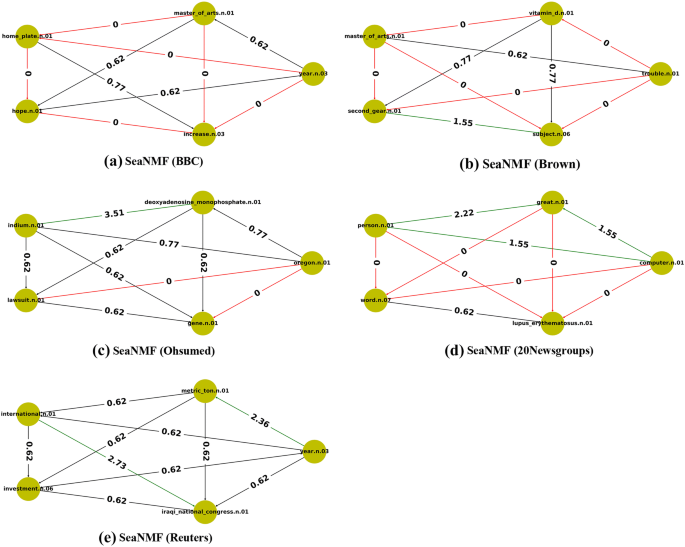

  

  Semantic network visualizations of the top term-topic obtained by SeaNMF model on all datasets, the line is colored in red if its degree is 0, green if its degree greater than 1 and otherwise black. The numbers in the line represent the Resnik semantic similarity of the term in the corpus

  Table 6 Discovered topics by the proposed method H4 and SeaNMF

  In contrast, to better understand the different performance of the SNNMF algorithms, we now turning to the dimensionality reduction approach. The main purpose of the dimensionality reduction methodologies is discussed in Sect. 3 is achieving the optimum solution to the semantic coherence topics over all datasets.

  SNNMF represents two semantic coherence types, local and global. The local semantic coherence is the semantic coherence (relation) between the topic (main term) and the other terms belonged to the same topic (in the same column). The global coherence is the semantic coherence (relation) among the terms in the same topic. The global semantic coherence in addition to the local semantic coherence effect on the overlaps between topic, which is in turn affects the accuracy of the recall of information. In addition, the global semantic coherence in addition to the local semantic coherence highlights the semantic contrast level in dataset. In short, Algorithm 2 works via the local semantic coherence. In contrast, Algorithm 4 works via the global semantic coherence.

  As we have seen, the experiments obtained in Table 5 face three cases for SNNMF algorithms.

  • Case 1, significant such as BBC (H4 = H2 > H1).

  • Case 2: not significant such as Ohsumed and Reuters (H4 = H2 = H1).

  • Case 3: decline such as 20 Newsgroups and Brown (H4 = H2 < H1).

  Case 1 (significant) In BBC H4 = H2 > H1, our proposed method is capable of generating more cohesive topics (significant) via Algorithm 2 but not improved by Algorithm 4 (useless). In other words, we can say SNNMF highlights a weak semantic contrast in BBC via the local semantic coherence.

  Case 2 (not significant) In Ohsumed and Reuters H4 = H2 = H1, our proposed method is capable of generating more cohesive topics (significant) via Algorithm 1 but not improved by Algorithms 2 and 4 (useless or not significant). In other words, we can say the dimensionality reduction that is used in SNNMF (Algorithms 2 and 4) is not a significant for the dataset that is built based on the semantic linguistics approach (no semantic contrast).

  Case 3 (decline) In 20 Newsgroups and Brown H4 = H2 < H1, our proposed method is capable of generating more cohesive topics (significant) via Algorithm 1 but decline by Algorithms 2 and 4. This means the topics in 20 Newsgroups and Brown contains many terms with a weak semantic relation. In other words, we can say SNNMF highlights a strong semantic contrast in 20 Newsgroups and Brown.

  In the more, Fig. 4 visualizes the top five terms in the top topic performed by SNNMF-H4 for all datasets. In addition, the lists of the top five terms in the top topic per dataset below in Table 6 to represents the semantic correlation among each other by Resnik (res).

  Fig. 4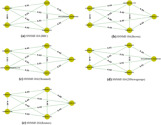

  

  Semantic network visualizations of the top term-topic obtained by SNNMF model on all datasets, the line is colored in red if its degree is 0, green if its degree greater than 1 and otherwise black. The numbers in the line represent the Resnik semantic similarity of the term in the corpus

  Notes: Overall, all results via Algorithm 4 (H4) are the same by the Algorithm 2 (H2). In other words, Algorithm 4 seems to be not significant for the semantic coherence topic. In facts, the generated topic vectors by the Algorithms 4 and 2 are not the same. later on, metrics based on statistical analysis will prove that.

• 2. Metrics based on statistical analysis In Table 5, we contrast the results of SNNMF strategies and the reference strategies, considering the NPMI metric. As we can see, our strategy achieves the single best results in 3 out of 5 results, tying with SeaNMF in the other 2 as the best method in terms of the quality of the discovered topics. To understand the different performance of SNNMF algorithms compared to SeaNMF in terms NPMI. Firstly, we should remember that the idea behind topic coherence is that a coherent topic will display terms that tend to occur in the same documents. In other words, the most likely words in a coherent topic should have high mutual information. The topic models with higher topic coherence are more interpretable topic models. NPMI measures this coherence.

  Reuters is the only datasets in which the test showed improvement NPMI via Algorithm 4 between the strategies. However, in this dataset, SNNMF outperforms SeaNMF considering all strategies. In other words, NPMI is improved by SNNMF-H4 in Reuters compared to SeaNMF and SNNMF Algorithms 2 and 1. We discussed before in semantic topic coherence that Reuters is the dataset that is built based on the semantic linguistics approach (no semantic contrast). We combine semantic coherence with a second metric NPMI. We can prove that Reuters is the dataset that is built based on the semantic linguistics approach (no semantic contrast). In addition, term NPMI highlights value by SNNMF-H4 more than SNNMF-H2 and SNNMF-H1. In addition, in terms NPMI highlights the max value by SNNMF-H4 in Reuters. This is point out the differentiate between term-topic vectors are generated by Algorithm 2 compared to Algorithm 4 in other words, H4 is not the same H2. This is highlighting the importance of the Algorithm 4. In contrast, Brown, and BBC only the only datasets in which the test showed improvement NPMI via Algorithm 1 between the strategies. However, in these datasets, SNNMF outperforms SeaNMF considering all strategies. Overall, Algorithm 1 generates a term-topic vectors with high range compared to Algorithms 2 and 4 sequentially, In addition to the semantic contrast dataset like BBC and Brown. With combining these factors leads to outperform NPMI of SNNMF-H1 compered to SNNMF-H2 and 4.

4.2.2 Qualitative evaluation

See Table 7.

Table 7 Topics by SNNMF and SeaNMF for Reuters dataset for k = 5, the word is colored in green if it shared between the two models, the row is highlighted colored in gray if its result is zero

Jaccard index is a name often used, for comparing similarity, dissimilarity, and distance of the data set. Measuring the Jaccard similarity coefficient between two data sets is the result of the division between the number of features that are common to all divided by the number of properties. For Jaccard similarity value in Table 7, the higher similarity values show increased topic dependency between two models. We observed, all topic dependency between the two models are weak.

4.3 Summary

With these experiments we can answer these questions. The first, what is the extent of impact semantic relations, and WSD terms on the topic-detection? By using the linguistics features (semantic relations, and WSD), SNNMF can discover the dataset which is its topic built based on the semantic linguistics approach (Table 5). The second, what is the impact of using the dimensionality reduction with the lexical semantic relations on the coherence topic? The dimensionality reduction by the lexical semantic relations improve the coherence topic (SS & NPMI) over the dataset which is non-semantic contrast such as Reuters.

5 Conclusion and future work

In this paper, we introduced a semantics non-negative matrix factorization (SNNMF) model to discover the topics for the texts. The proposed model utilized the lexical semantic correlations in addition the WSD in the training, the semantic correlations between the terms learned from the lexical semantic by Resnik, which was demonstrated to be effective for revealing word semantic relationships. We used semantic dimensionality reduction algorithms to solve our SNNMF model. In addition, it conjugates into a representation semantic information. We compared the performance of our model with other state-of-the-art method on five real-world datasets. The quantitative evaluations demonstrated that our model outperformed the other method with respect to widely used metrics such as the semantic topic coherence and NPMI. The qualitative results shown that the topics discovered by SNNMF are meaningful and their top terms are more semantically correlated. Hence, we concluded that the proposed SNNMF is an effective topic model for texts.

In the future work, we plan to use the dynamic word embedding (word embeddings techniques that take into consideration the context of the word) such as BERT for semantic text representation, we will develop this model for topic tracking.

References

Priyadarshini R, Tamilselvan L, Khuthbudin T, Saravanan S, Satish S (2015) Semantic retrieval of relevant sources for large scale virtual documents. Procedia Comput Sci 54:371–379
Alghamdi R, Alfalqi K (2015) A survey of topic modeling in text mining. Int J Adv Comput Sci Appl: IJACSA 6(1):147–153
Boyd-Graber J, Blei D, Zhu X (2007) A topic model for word sense disambiguation. In: Proceedings of the 2007 joint conference on empirical methods in natural language processing and computational natural language learning (EMNLP-CoNLL)
Wang J, Bansal M, Gimpel K, Ziebart BD, Clement TY (2015) A sense-topic model for word sense induction with unsupervised data enrichment. Trans Assoc Comput Linguist 3(1):59–71
Lee S, Masoud M, Balaji J, Belkasim S, Sunderraman R, Moon SJ (2017) A survey of tag-based information retrieval. Int J Multimed Inf Retr 6(2):99–113
Vorontsov K, Potapenko A (2014) Tutorial on probabilistic topic modeling: additive regularization for stochastic matrix factorization. In: International conference on analysis of images, social networks and texts. Springer, Cham, pp 29–46
Belford M, MacNamee B, Greene D (2016) Ensemble topic modeling via matrix factorization. In: 24th Irish conference on artificial intelligence and cognitive science (AICS’16), Dublin, Ireland, 20–21 September 2016, vol 1751. CEUR workshop proceedings
Belford M, Mac Namee B, Greene D (2018) Stability of topic modeling via matrix factorization. Expert Syst Appl 91:159–169
ur Rehman MH, Liew CS, Abbas A, Jayaraman PP, Wah TY, Khan SU (2016) Big data reduction methods: a survey. Data Sci Eng 1(4):265–284
Ramkumar AS, Poorna B (2016) Text document clustering using dimension reduction technique. Int J Appl Eng Res 11(7):4770–4774
Jindal R, Taneja S (2016) WordNet based semantic approach for dimension reduction in multi label text documents. IJCTA 9(40):267–274
Yan J, Hu J (2009) Text semantic representation. In: Liu L, Özsu MT (eds) Encyclopedia of database systems. Springer, Boston
Handler A (2014) An empirical study of semantic similarity in WordNet and Word2Vec. Master dissertation, Columbia University
Kabir KL, Alam FF, Islam AB (2019) Word embeddings for semantic resemblance of substantial text data. In: Smart systems and IoT: innovations in computing: proceeding of SSIC 2019, vol 141, p 303
Levy O, Goldberg Y, Dagan I (2015) Improving distributional similarity with lessons learned from word embeddings. Trans Assoc Comput Linguist 3:211–225
Saedi C, Branco A, Rodrigues J, Silva J (2018) Wordnet embeddings. In: Proceedings of the third workshop on representation learning for NLP, pp 122–131
Clark A, Fox C, Lappin S (eds) (2013) The handbook of computational linguistics and natural language processing. Wiley, Hoboken
Dongsuk O, Kwon S, Kim K, Ko Y (2018) Word sense disambiguation based on word similarity calculation using word vector representation from a knowledge-based graph. In: Proceedings of the 27th international conference on computational linguistics, pp 2704–2714
Vial L, Lecouteux B, Schwab D (2019) Sense vocabulary compression through the semantic knowledge of WordNet for neural word sense disambiguation. arXiv:1905.05677
Zhu X, Yang X, Huang Y, Guo Q, Zhang B (2019) Measuring similarity and relatedness using multiple semantic relations in WordNet. Knowl Inf Syst. https://doi.org/10.1007/s10115-019-01387-6
Jipeng Q, Zhenyu Q, Yun L, Yunhao Y, Xindong W (2019) Short text topic modeling techniques, applications, and performance: a survey. arXiv:1904.07695
Schneider J, Vlachos M (2018) Topic modeling based on keywords and context. In: Proceedings of the 2018 SIAM international conference on data mining. Society for Industrial and Applied Mathematics, pp 369–377
Zhao H, Du L, Buntine W, Liu G (2018) Leveraging external information in topic modelling. Knowl Inf Syst 61(2):661–693
Li S, Pan R, Zhang Y, Yang Q (2016) Correlated tag learning in topic model. In: Proceedings of the thirty-second conference on uncertainty in artificial intelligence. AUAI Press, pp 457–466
Allahyari M, Kochut K (2016) Semantic tagging using topic models exploiting Wikipedia category network. In: 2016 IEEE tenth international conference on semantic computing (ICSC). IEEE, pp 63–70
Xu K, Qi G, Huang J, Wu T (2017) Incorporating Wikipedia concepts and categories as prior knowledge into topic models. Intell Data Anal 21(2):443–461
Pedersen T (2010) Information content measures of semantic similarity perform better without sense-tagged text. In: Human language technologies: the 2010 annual conference of the North American chapter of the Association for Computational Linguistics. Association for Computational Linguistics, pp 329–332
Pfeifer D, Leidner JL (2019) Topic grouper: an agglomerative clustering approach to topic modeling. In: European conference on information retrieval. Springer, Cham, pp 590–603
Kuang D, Choo J, Park H (2015) Nonnegative matrix factorization for interactive topic modeling and document clustering. In: Celebi ME (ed) Partitional clustering algorithms. Springer, Cham, pp 215–243
Lee DD, Seung HS (1999) Learning the parts of objects by non-negative matrix factorization. Nature 401:788–791
Shi T, Kang K, Choo J, Reddy CK (2018) Short-text topic modeling via non-negative matrix factorization enriched with local word-context correlations. In: Proceedings of the 2018 World Wide Web conference on World Wide Web. International World Wide Web Conferences Steering Committee, pp 1105–1114
Chen Y, Zhang H, Liu R, Ye Z, Lin J (2018) Experimental explorations on short text topic mining between LDA and NMF based Schemes. Knowl Based Syst 163:1–13
Viegas F, Luiz W, Gomes C, Khatibi A, Canuto S, Mourão F, Salles T, Rocha L, Gonçalves MA (2018) Semantically-enhanced topic modeling. In: Proceedings of the 27th ACM international conference on information and knowledge management. ACM, pp 893–902
Hong HK, Kim GW, Lee DH (2018) Semantic tag recommendation based on associated words exploiting the interwiki links of Wikipedia. J Inf Sci 44(3):298–313
Viegas F, Canuto S, Gomes C, Luiz W, Rosa T, Ribas S, Gonçalves MA (2019) CluWords: exploiting semantic word clustering representation for enhanced topic modeling. In: Proceedings of the twelfth acm international conference on web search and data mining. ACM, pp 753–761
Martin F, Johnson M (2015) More efficient topic modelling through a noun only approach. In: Australasian language technology association workshop 2015, p 111
Guo W, Diab M (2011) Semantic topic models: combining word distributional statistics and dictionary definitions. In: Proceedings of the conference on empirical methods in natural language processing. Association for Computational Linguistics, pp 552–561
Nguyen DQ, Billingsley R, Du L, Johnson M (2018) Improving topic models with latent feature word representations. arXiv:1810.06306
Nikolenko SI (2016) Topic quality metrics based on distributed word representations. In: Proceedings of the 39th international ACM SIGIR conference on research and development in information retrieval. ACM, pp 1029–1032
O’Callaghan D, Greene D, Carthy J, Cunningham P (2015) An analysis of the coherence of descriptors in topic modeling. Expert Syst Appl 42(13):5645–5657
Wallach HM, Murray I, Salakhutdinov R, Mimno D (2009) Evaluation methods for topic models. In: Proceedings of the 26th annual international conference on machine learning. ACM, pp 1105–1112
Fang A, Macdonald C, Ounis I, Habel P (2016) Topics in tweets: a user study of topic coherence metrics for Twitter data. In: European conference on information retrieval. Springer, Cham, pp 492–504
Newman D, Lau JH, Grieser K, Baldwin T (2010) Automatic evaluation of topic coherence. In: Human language technologies: the 2010 annual conference of the North American chapter of the Association for Computational Linguistics. Association for Computational Linguistics, pp 100–108
Röder M, Both A, Hinneburg A (2015) Exploring the space of topic coherence measures. In: Proceedings of the eighth ACM international conference on Web search and data mining. ACM, pp 399–408
Nikolenko SI, Koltcov S, Koltsova O (2017) Topic modelling for qualitative studies. J Inf Sci 43(1):88–102
Blair SJ, Bi Y, Mulvenna MD (2019) Aggregated topic models for increasing social media topic coherence. Appl Intell. https://doi.org/10.1007/s10489-019-01438-z
Peng C, Kang Z, Hu Y, Cheng J, Cheng Q (2017) Nonnegative matrix factorization with integrated graph and feature learning. ACM Trans Intell Syst Technol: TIST 8(3):42
Izquierdo R, Postma M, Vossen P (2015) Topic modeling and word sense disambiguation on the Ancora corpus. Procesamiento del Lenguaje Natural 55:15–22
Author information
Authors and Affiliations
Corresponding author
Ethics declarations
Conflict of interest
On behalf of all authors, the corresponding author states that there is no conflict of interest.
Additional information
Publisher's Note
Springer Nature remains neutral with regard to jurisdictional claims in published maps and institutional affiliations.
Rights and permissions
About this article
Cite this article
Gadelrab, F.S., Haggag, M.H. & Sadek, R.A. Novel semantic tagging detection algorithms based non-negative matrix factorization. SN Appl. Sci. 2, 54 (2020). https://doi.org/10.1007/s42452-019-1836-y
Received:
Accepted:
Published:
DOI: https://doi.org/10.1007/s42452-019-1836-y