
Abstract
This paper presented two decentralized neuro-fuzzy controllers to control the level in lower two tanks in nonlinear quadruple tank system (QTS). The controllers are designed based on adaptive neuro-fuzzy inference system technique. The relation between inputs/outputs was proved using relative gain array, and then, we can divide the quadruple tank system into two subsystems and control each of them separately. The first controller is a neuro-fuzzy inverse nonlinear (NFIN) model, which predicts the voltage required to control the level to track the referred one. So, the voltage was fed to neuro-fuzzy forward nonlinear model (NFFN) to obtain the desired level. The second is neuro-fuzzy nonlinear gain scheduling PI controller, which is designed to control the nonlinear QTS at any operating point. The results show that the NFIN controller has a more accurate tracking level and less computational time in both minimum and non-minimum phases.
1 Introduction
Quadruple tank system (QTS) is broadly utilized as a part of a chemical and petroleum process. The framework is extremely unpredictable to control because of its nonlinearity and the higher connection between inputs/outputs. The levels of fluid in the two lower tanks should be controlled and managed to achieve a specific reference level.
Examining this issue can be taken care of by numerous analyses for both minimum and non-minimum phases. The contrasts between minimum and non-minimum phase conduct for the QTS have been considered and controlled by the decentralized PI controller by [1, 2].
Advanced control theory and techniques, for example, predictive control, genetic algorithm, sliding mode and neuro-fuzzy controllers can be designed to control QTS with more exact outcomes than traditional control strategies. In [4], a multivariable predictive PID controller was executed on a four-tank system to modify the transmission zero to work in minimum and non-minimum phases. Kayacan and Kaynak [5] proposed a grey prediction-based fuzzy PID controller, while [6] presented a basic genetic algorithm (GA) technique for online auto tuning proportional–integral–derivative (PID) parameters to control the fluid level in QTS.
In [7] in view of the Takagi–Sugeno–Kang (TSK) piecewise direct fuzzy modeling approach, a long-range predictive control calculation for nonlinear QTS forms working over a wide range is proposed.
In [7] in view of the Takagi–Sugeno–Kang (TSK) piecewise direct fuzzy modeling approach, a long-range predictive control calculation for nonlinear QTS forms working over a wide range is proposed.
Both the decentralized predictive and proportional–integral (PI) controllers are planned by [8] for the QTS framework. A decoupling-based agreeable conveyed multi-parametric model predictive controller (MPC) is proposed. The controllers are subjected to reference tracking and disturbance dismissal, and the execution measures are looked at.
In the HD-MPC research, eight diverse MPC controllers were connected to the four-tank process plant. These controllers depended on various models and suppositions and give a wide perspective of the diverse distributed MPC plans [9].
Bristol [10] displayed an adequacy controller planned in view of a mix of state feedback and a sliding mode controller for four-tank system utilizing fuzzy logic for non-minimum phase mode. The sliding mode control (SMC) strategy is utilized to accomplish a quick transient reaction, while the state feedback controller (SFC) can give zero stationary state errors.
Many of the researchers use the linear mathematical model to design a controller. The novelty of this paper is to use data of the nonlinear quadruple liquid-level tanks to create the neuro-fuzzy forward nonlinear (NFFN) model for quadruple tank system. In addition, the neuro-fuzzy inverse nonlinear (NFIN) model has been designed as a nonlinear controller and examined for different conditions for both minimum and non-minimum phases. Also, the required operating points for levels in tank 3, tank 4 and the voltages to both pump 1 and pump 2 from known levels in tank 1 and tank 2 are derived and implemented in neuro-fuzzy gain scheduling PI (NFGSPI) controller. The proposed controllers improve the performance of a multi variable nonlinear liquid-level system.
This paper is constructed as follow: Section 3 presents specification of quadruple tank process, nonlinear and linear model. Section 3 presents the neuro-fuzzy controller framework. The neuro-fuzzy gain scheduling PI controller is introduced in Sect. 4. Results and simulation are displayed in Sect. 5. Lastly, Sect. 6 is the conclusion.
2 Quadruple tank processes
2.1 System description
The quadruple tank system (QTS) is used to illustrate many concepts in MIMO systems. The quadruple tank laboratory equipment consists of four interacting tanks (1, 2, 3 and 4), two-way valves, two pumps and a reservoir as shown in Fig. 1.

Quadruple tank system
Tank 1 and tank 2 are in the lower, while tank 3 and 4 in the upper. The flow is delivering to tanks 1 and 3 from a reservoir by pump 1, while pump 2 sucks the flow and delivers it to the other tanks. The two-way valves after each pumping are used to divide the flow to lower and upper tanks by a factor \(\gamma_{i} \,{\text{and}}\,\left( {1 - \gamma_{i} } \right)\) which is fixed during the experiment. The input voltages v1 and v2 to the pumps are varied during the experiment according to the required controlled outputs (the liquid levels in the lower tanks 1 and 2). A reservoir is used to accumulate the outgoing water from tank 1 and tank 2 and is present in the bottom.
The operation of QTS can be in two phases: minimum phase and non-minimum phase. The system starts operating in non-minimum phase when the fraction of liquid entering the lower tanks is less than that of upper tanks. Otherwise, the system starts operating in minimum phase when the fraction of liquid entering the upper tanks is less than that of lower tanks. The minimum phase and non-minimum phase can be achieved as:
2.2 Nonlinear quadruple tank model
The nonlinear model of QTS is based on mass balances for each tank and the differential equations are formulated as:
where Ai is the cross section of tank i, i = (1, 2, 3, 4); ai is the open cross section of the outlet line valve; hi is the water level; \(v_{i}\) is the voltage applied to pump; \(k_{i} v_{i}\) is the flow from the pump; γi is the position of the valve; and g is the gravitational constant.
2.3 Linear model
The linearized state-space model about operating point is given by Eq. (5).
The time constants Ti are
The required operating points for levels in tank 3, tank 4 and the voltages to both pump 1 and pump 2 from known levels in tank 1 and tank 2 are given by Eq. (6).
According to Eqs. (6a–6b), a MATLAB program is created to calculate the operating point for a level in tanks 3 and 4, and also the steady-state voltage inputs to pump 1 and pump 2.
The parameter values and steady-state operating points of the process are listed in Table 1 [3].
The transfer function matrix is given in Eq. (7) for minimum phase and non-minimum phase operating points.
2.4 Decentralized by relative gain array (RGA)
Decentralized control is an entrenched way to compact with control the multi-input-multi-output MIMO plants. To outline a decentralized controller, matching between input–output must be dictated by RGA. The method exchanges of open-loop and closed-loop control structures are assessed for all conceivable input/output pairings. The array will be a matrix with one row for each output variable and one column for each input variable in the MIMO framework [11]. A few principles for blending determination can be expressed: the variable pairings comparing to positive relative gains as near unity as conceivable ought to be favored. Negative relative gain much longer than unity ought to be evaded.
The relative gain array is defined as follow:
where × denotes the element-by-element product of the two matrices.
(RGA) the concept is employed to QTS to determine the input–output pairing for both minimum phase and non-minimum phase.
For minimum phase system, λ11 is obtained as 1.4, so the pairing is determined as y1–u1 and y2–u2. But for the non-minimum phase system, λ11 is obtained as − 0.64, so the suitable pairing is found as y1–u2 and y2–u1.
3 Neuro-fuzzy nonlinear control system
Neuro-fuzzy model is a nonparametric model for emulating quadruple-level tank system. It is faster than the numerical model for keeping the error moderately little. The neuro-fuzzy is a utilization of ANFIS (adaptive neuro-fuzzy inference system). ANFIS demonstrates to utilize neuro-adaptive learning strategies, which are like those of neural systems, initially exhibited by Jang [12].
A block diagram of the decentralized neuro-fuzzy control for a quadruple liquid-level framework is shown in Fig. 2. The framework incorporates two subsystems: one for control level in tank 1 and the other for control level in tank 2. Every subsystem contains neuro-fuzzy forward nonlinear (NFFN) model in arrangement with a neuro-fuzzy inverse nonlinear (NFIN) controller. MATLAB programming is utilized to make the forward and inverse model and simulate the control framework.

Simulation of decentralized neuro-fuzzy control system
3.1 Neuro-fuzzy forward nonlinear (NFFN) model
3.1.1 Training forward nonlinear model
The initial step in preparing NFFN pattern is to collect an arrangement of input/output data set. Given collected informational data, ANFIS can acquire an ideal dispersion of membership function by utilizing back propagation formula.
The QTS is isolated into two subsystems as indicated by the consequences of RGA. From data obtained from a test work, forcing arbitrary voltages in the vicinity of 0 and 10 V to acquire 2000 data samples which separated to 1000 focuses for training phase and residue 1000 samples focuses utilized for checking phase. Each NFFN subsystem has two inputs; the voltage input signal v(k), one sample delay of level yield h(k) and a solitary output h(k+1). Table 2 demonstrates the input/output for all loops.
Differentiation between NFFN model and theoretical model is shown in Figs. 3 and 4 for both minimum and non-minimum cases. Figures 5 and 6 demonstrate the inaccuracy between two models. It is noticed that the NFFN model and theoretical model are near each other, with a little measure of error which is under ± 2 mm in level in tank 1 and about ± 1 mm in level in tank 2 for the two stages.

NFFN and experimental nonlinear model for minimum phase

NFFN and experimental nonlinear model for non-minimum phase

The error between NFFN and experimental nonlinear models for minimum phase

The error between NFFN and experimental nonlinear models for non-minimum phase
3.1.2 Neuro-fuzzy inverse nonlinear (NFIN) model
Control of level in QTS is very important for all applications. The system is nonlinear and very complicated to control due to multiple variables and interaction between inputs and outputs.
Decentralized technique selects the input–output pairing to be directly controlled; then, we can control the applied voltage which can directly control the flow to tanks through pumps. To achieve that, we must build an inverse model. It predicts the voltage required to be applied to the pump to produce the desired level (reference level).
Inverse learning is an application of ANFIS used for designing a neuro-fuzzy inverse model to be operated as a controller. The design process involves two phases: learning phase for which an online technique is used to train the controller. The controller inputs are the tank reference level at current time step hd(k), the tank level at the next time step h(k+1), while the voltage at current time step v(k) is the output.
The data obtained from experimental work is used to train the (NFNI) model as similar to NFFN model. Each input and output is with ten membership function and ten rules. The application phase has been used to generate the required level (reference level). In this phase, the inputs to NFNI controller are the level of the tank at current time step and reference level at the next time step. Figures 7 and 8 show the voltage predicted by NFNI model to track the desired level for both phases.

The predicted voltage by NFNI model to track the desired level (minimum phase)

The predicted voltage by NFNI model to track the desired level (non-minimum phase)
4 Neuro-fuzzy gain scheduling PI controller
Gain scheduling is a linear parameter varying feedback regulator whose parameters changed as a function of operating conditions. Then, we use linear behavior controllers for control nonlinear system.
The proposed neuro-fuzzy gain scheduling PI (NFGSPI) controller-based design approach can be described as follows [13]:
-
1.
Define the domain of interest in the state-space and set operating points within the domain of interest.
-
2.
For each of the operating points, find the linearized model of the quadruple tank system as in Eq. (7) and then determine the PI controller parameters based on reference input.
-
3.
Use data from step 2 to train an NFGSPI controller using ANFIS technique.
ANFIS helps to construct and optimize the shape of MFs that can interpolate the gains with respect to several operating points in NFGSPI.
Because the ANFIS has a single output, then two FGSPIs have been constructed for each subsystem: one to determine gain kp and the other for obtaining gain ki.
-
4.
Gains kp, ki which are outputs from FGSPI apply to the classical PI controller to generate the control signal. The proposed FGSPI controller scheme is shown in Fig. 9.
Fig. 9 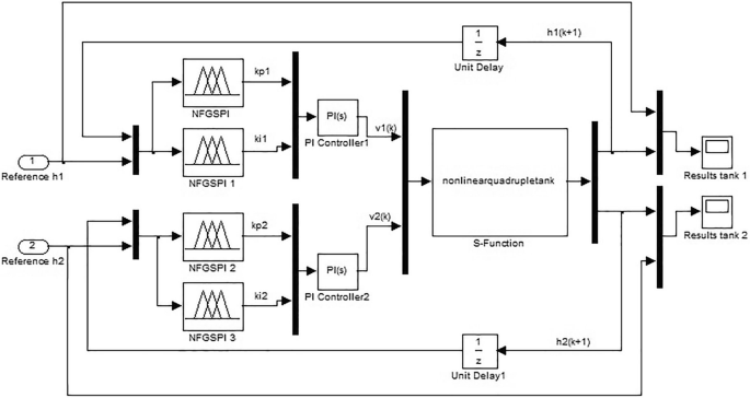
Simulation of a neuro-fuzzy gain scheduling PI controller system

5 Results
The two NF nonlinear controllers are constructed and simulated by utilizing MATLAB programming. The NF nonlinear controllers are executed for both the minimum and non-minimum cases. The framework needs to track the levels in tank 1 and tank 2 as indicated for different cases appeared in Table 3.
Figures 10, 11, 12, 13, 14, 15, 16 and 17 demonstrate the fluid-level reaction of utilizing NFIN and NFGSPI controllers for tank 1 and 2 separately. It is noticed that the two controllers can track the reference level for the two cases. Anyway the NFIN controller demonstrates a superior steady-state execution as contrasted to NFGSPI controller.

Predicted and a reference level in tanks 1 and 2 by NFNI controller for minimum phase (case 1)

Predicted and a reference level in tanks 1 and 2 by NFNI controller for non-minimum phase (case 1)

Predicted and a reference level in tanks 1 and 2 by NFNI controller for minimum phase (case 2)

Predicted and a reference level in tanks 1 and 2 by NFNI for non-minimum phase (case 2)

Predicted and a reference level in tanks 1 and 2 by NFGSPI controller for minimum phase (case 1)

Predicted and a reference level in tanks 1 and 2 by NFGSPI controller for non-minimum phase (case 1)

Predicted and a reference level in tanks 1 and 2 by NFGSPI controller for minimum phase (case 2)

Predicted and a reference level in tanks 1 and 2 by NFGSPI controller for non-minimum phase (case 2)
Besides, NFIN did not have to process the dynamical nonlinear conditions as NFGSPI. Additionally, in the non-minimum phase which is more difficult to control, NFIN can get phenomenal and exact outcomes than NFGSPI.
6 Conclusion
This paper presents a NF decentralized controllers for nonlinear quadruple tank system. The novelty of this paper is to use data from experimental test to create a forward neuro-fuzzy (FNF) model, which can describe the system with high accuracy and coincides with the experimental data. Then, two controllers are presented: the first is NFIN model which used as a controller and the second is NFGSPI controller which built in light of planning PI controller picks up gains at various operating points. Both of the two nonlinear controllers have been examined by MATLAB programming for different conditions for both minimum and non-minimum phases. Simulation results show that the decentralized NFIN is effective than NFGSPI controller and has less response time and can track the desired level with minimum error approximately 2 mm. Thus, the proposed decentralized NFIN presented in this paper is superior in controlling nonlinear processes.
References
Sombría JC, Moreno JS, Visioli A, Bencomo SD (2012) Decentralised control of a quadruple tank plant with a decoupled event-based strategy. In: IFAC proceedings volumes (IFAC-PapersOnline), 2(PART 1), pp 424–429
Suja M, Thyagarajan T (2008) Design of decentralized fuzzy controllers for quadruple tank process. Int J Comput Sci Netw Secur 8(11):163–168
Saeed Q, Uddin V, Katebi R (2010) Multivariable predictive PID control for quadruple tank. World Acad Sci Eng Technol 1(1):658–663
Kayacan E, Kaynak O (2009) An adaptive grey PID-type fuzzy controller design for a non-linear liquid level system. Trans Inst Meas Control 31(1):33–49
Teng TK, Shieh JS, Chen CS (2003) Genetic algorithms applied in online autotuning PID parameters of a liquid-level control system. Trans Inst Meas Control 25(5):433–450
Mahfouf M, Kandiah S, Linkens DA (2001) Adaptive estimation for fuzzy TSK model-based predictive control. Trans Inst Meas Control 23(1):31–50
Kirubakaran V, Radhakrishnan TK, Sivakumaran N (2014) Distributed multiparametric model predictive control design for a quadruple tank process. Meas J Int Meas Confed 47(1):841–854
Alvarado I, Limon D, Muñoz De La Peña D, Maestre JM, Ridao MA, Scheu H, Espinosa J (2011) A comparative analysis of distributed MPC techniques applied to the HD-MPC four-tank benchmark. J Process Control 21(5):800–815
Mirakhorli E, Farrokhi M (2011) Sliding-mode state-feedback control of non-minimum phase quadruple tank system using fuzzy logic. In: IFAC proceedings Volumes (IFAC-PapersOnline), 18(PART 1), pp 13546–13551
Bristol EH (1966) On a new measure of interactions for multivariable process control. J IEEE Trans Autom Control 11:133–134
Jang JSR (1993) ANFIS-adaptive-network based fuzzy inference system. IEEE Trans Syst Man Cybern 23:665–684
Jang JSR (1997) Neuro-fuzzy and soft computing: a computational and learning and machine intelligence. Prentice Hall, New Jersey
Zhang J (2001) A nonlinear gain scheduling control strategy based on neuro-fuzzy networks. Ind Eng Chem Res 40(14):3164–3170
Author information
Authors and Affiliations
Corresponding author
Ethics declarations
Conflict of interest
The authors declare that they have no conflict of interest.
Rights and permissions
About this article

Cite this article
Eltantawie, M.A. Decentralized neuro-fuzzy controllers of nonlinear quadruple tank system. SN Appl. Sci. 1, 39 (2019). https://doi.org/10.1007/s42452-018-0029-4
Received:
Accepted:
Published:
DOI: https://doi.org/10.1007/s42452-018-0029-4