Simulation of Diffusion Advection Phenomena with Retardation and Source/Sink Terms Using a Series of Completely Mixed Reactors

Abstract

In this research, pollution transport in a 1-D domain with a source/sink and a retardation term is simulated using a series of completely mixed reactors. It is shown that as the volume of these reactors approaches zero, the governing equation of the system becomes identical to the advection diffusion partial differential equation. By application of mass balance to a finite number of completely mixed reactors, a set of ordinary differential equations which is equivalent to spatially discretized form of the equation is obtained in a completely natural and intuitive way. More importantly, the proposed innovative model can offer a conceptual insight into pollution transport phenomena and is flexible to any change for different problems.

1 Introduction

Pollution transport is one of the most significant problems in environmental engineering and mainly takes place as a result of advection, diffusion, and reactions in rivers. Simulation of such problems is mostly concerned with solving differential equations. Obtaining an analytical solution is not always possible, and therefore numerical methods are mostly used to solve these equations. On the other hand, a comprehensive model which is able to simulate the advection–diffusion process in a river physically, based on a familiar concept such as mass balance, may yield to establishment of a more well-defined scheme rather than those presented by numerical methods, typically. As physical sense can be highlighted in the model, implementing new initial and boundary conditions as well as the other desirable changes in the problem statement can be carried out in a more obvious framework.

Application of mass balance in completely mixed reactors for transport simulation has been used extensively by researchers (Hill and Root 2014; Carberry 2001; Jakobsen 2008; Mann 2009; Salmi et al. 2010; Davis and Davis 2012). Advection–diffusion simulation has been studied using feedforward and back-feed reactors by Chapra (1997). Dispersion effects have been addressed by Metcalf and Eddy (Burton et al. 2014). Effects of chemical reactions in pollutants fate using completely mixed reactors have been investigated by Hessel et al. (2004) and have been employed to indoor air quality simulations by Hayes (1991) and WHO (2015). As far as the authors are concerned, diffusion of pollution by completely mixed reactors has not been simulated using flow rates to/from a reactor in feedforward and back-feed systems.

In this study, it is shown that application of mass balance to a series of reactors transforms the transport equation into a system of linear equations. This transformation is equivalent to application of numerical methods for solving the governing partial differential equation (PDE) of mass transport. Existence of source/sink and reactions has also been formulated. Furthermore, these formulations are verified using several examples and comparing the results with the analytical solution.

2 Methodology and Formulation

2.1 Model Construction

It is assumed that pollution transport in a 1-D river may be simulated by a series of completely mixed reactors. In this model, each reactor is connected to its left and right reactors via pipes. Water storage and reactions take place in these reactors, and driving forces for pollution transport (i.e., diffusion and advection) are provided by implementing pumps.

2.1.1 Diffusion Simulation

Diffusion is a type of random motion where molecular movements to left and right have the same probability. In order to model diffusion in the proposed model, an arbitrary reactor (e.g., reactor i, shown in Fig. 1a) is connected to its adjacent reactors at its left and right (reactors i − 1 and i + 1) by two identical pumps: i, i + 1. Using this concept, transmission of pollution to left and right with the same probability is allowed. This process is applied for all other reactors, as shown in Fig. 1a, to model diffusion process in the whole domain. As pumps start working simultaneously, pollution transports from time 0 onward.

Fig. 1

a Simulation of diffusion using completely mixed reactors in series. b Simulation of advection using completely mixed reactors in series. c Simulation of diffusion–advection in a 1-D domain using completely mixed reactors

2.1.2 Advection Simulation

Advection is the transport of pollution by bulk flow in river. In order to model advection (form left to the right part of the system), each reactor is connected to its right reactor via a pipe. The driving force for advection is provided by implementing a pump at downstream (the most right reactor) having a flow rate of Q_Adv (Fig. 1b). This layout allows the bulk transport of pollution from the left to the right of the system. Pollution concentration in the advective pipes is assumed to vary linearly.

2.1.3 Diffusion–Advection Simulation

By combination of the two mentioned systems, diffusion–advection may be modeled using a series of completely mixed reactors as shown in Fig. 1c.

2.2 Governing Equation

In order to derive the governing partial differential equation of the proposed model, it is assumed that the model consists of infinitely small reactors with a volume of dV. Since pollution varies linearly in the advective pipes, the concentration of pollution in these pipes is assumed to be the average of both their end concentrations. Mass balance equation for an interior reactor i shown in Fig. 2a is written as:

$$\dot{m}_{\text{in}} - \dot{m}_{\text{out}} = \frac{{{\text{d}}m}}{{{\text{d}}t}}.$$

(1)

Fig. 2

a An element used for deriving the governing PDE of the model. b Discretized simulation of a 1-D domain using completely mixed reactors for obtaining the discretized governing equation of the model

Substituting QC for ṁ yields:

$$\dot{m}^{\text{D}}_{\text{in}} = Q_{\text{D}} \left( {C - \frac{\partial C}{\partial x}{\text{d}}x + \frac{1}{2}\frac{{\partial^{2} C}}{{\partial x^{2} }}{\text{d}}x^{2} } \right) + Q_{\text{D}} \left( {C + \frac{\partial C}{\partial x}{\text{d}}x + \frac{1}{2}\frac{{\partial^{2} C}}{{\partial x^{2} }}{\text{d}}x^{2} } \right)$$

(2)

$$\dot{m}^{\text{D}}_{\text{out}} = 2Q_{\text{D}} C$$

(3)

$$\dot{m}^{\text{Adv}}_{\text{in}} = Q_{\text{A}} \left( {\bar{C}_{\text{Left}} } \right)$$

(4)

$$\dot{m}^{\text{Adv}}_{\text{out}} = Q_{\text{A}} \left( {\bar{C}_{\text{Right}} } \right).$$

(5)

Simplification of the above equations results in:

$$\begin{aligned} & Q_{\text{D}} \left( {C - \frac{\partial C}{\partial x}{\text{d}}x + \frac{1}{2}\frac{{\partial^{2} C}}{{\partial x^{2} }}{\text{d}}x^{2} } \right) - 2Q_{\text{D}} C + Q_{\text{D}} \left( {C + \frac{\partial C}{\partial x}{\text{d}}x + \frac{1}{2}\frac{{\partial^{2} C}}{{\partial x^{2} }}{\text{d}}x^{2} } \right) + \\ & Q_{\text{A}} \left( {\bar{C}_{\text{Left}} } \right) - Q_{\text{A}} \left( {\bar{C}_{\text{Right}} } \right) = \frac{\partial C}{\partial t}{\text{d}}V \to \\ & Q_{\text{D}} \left( {C - \frac{\partial C}{\partial x}{\text{d}}x + \frac{1}{2}\frac{{\partial^{2} C}}{{\partial x^{2} }}{\text{d}}x^{2} } \right) - 2Q_{\text{D}} C + Q_{\text{D}} \left( {C + \frac{\partial C}{\partial x}{\text{d}}x + \frac{1}{2}\frac{{\partial^{2} C}}{{\partial x^{2} }}{\text{d}}x^{2} } \right) + \\ & Q_{\text{A}} \left( {C - \frac{1}{2}\frac{\partial C}{\partial x}{\text{d}}x + \frac{1}{4}\frac{{\partial^{2} C}}{{\partial x^{2} }}{\text{d}}x^{2} } \right) - Q_{\text{A}} \left( {C + \frac{1}{2}\frac{\partial C}{\partial x}{\text{d}}x + \frac{1}{4}\frac{{\partial^{2} C}}{{\partial x^{2} }}{\text{d}}x^{2} } \right) = \frac{\partial C}{\partial t}{\text{d}}V \\ \end{aligned}$$

(6)

Simplification of Eq. (6) results in:

$$\left( {\frac{{Q_{\text{D}} {\text{d}}x^{2} }}{{{\text{d}}V}}} \right)\frac{{\partial^{2} C}}{{\partial x^{2} }} - \left( {\frac{{Q_{\text{A}} {\text{d}}x}}{{{\text{d}}V}}} \right)\frac{\partial C}{\partial x} = \frac{\partial C}{\partial t}{\text{d}}V$$

(7)

which shows that the governing equation for the proposed model is identical to the diffusion advection equation.

2.3 Discretization of the Governing Equation

In order to solve Eq. (7), one may use numerical methods to discretize this equation both spatially and temporally. In this research, however, a new procedure is followed for spatially discretizing Eq. (7). Writing mass balance equation for an arbitrary reactor (i), shown in Fig. 2b, yields:

$$Q_{\text{Diff}} C_{i - 1} - Q_{\text{Diff}} 2C_{i} + Q_{\text{Diff}} C_{i + 1} + Q_{\text{Adv}} \left( {\frac{{C_{i - 1} + C_{i} }}{2}} \right) - Q_{\text{Adv}} \left( {\frac{{C_{i} + C_{i + 1} }}{2}} \right) = \frac{{\partial C_{i} }}{\partial t}V_{i} .$$

(8)

Simplification of Eq. (8) yields:

$$\frac{{Q_{\text{Diff}} }}{{V_{i} }}\left( {C_{i - 1} - 2C_{i} + C_{i + 1} } \right) - \frac{{Q_{\text{Adv}} }}{{V_{i} }}\left( {\frac{{C_{i + 1} - C_{i - 1} }}{2}} \right) = \frac{{{\text{d}}C_{i} }}{{{\text{d}}t}}.$$

(9)

Application of Eq. (9) to all interior nodes yields a system of linear first-order differential equations which leads to closure when considering the boundary nodes. The time derivative in Eq. (9) and similar equations may be evaluated using forward, backward or Crank–Nicolson finite difference schemes.

2.4 Boundary Nodes

In order to write mass balance equation for boundary reactors, two types of boundaries are investigated in this research: infinite source and impermeable boundary.

• Infinite source: when a boundary is an infinite source such as lakes, concentration in this boundary is specified and constant over time (Fig. 3a).

  Fig. 3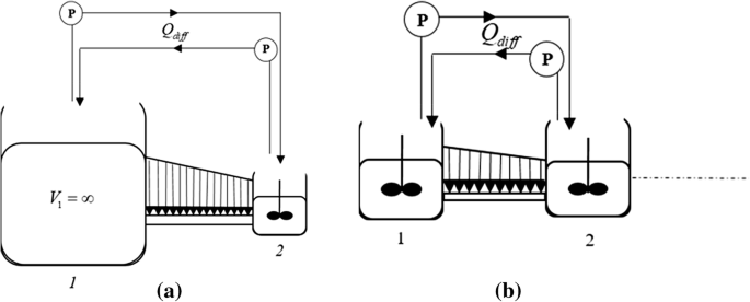

  

  a Simulation of an infinite source (Dirichlet boundary condition) using the proposed model. b Simulation of an impermeable boundary conditions by the proposed model

  In order to model this boundary, the reactor at that boundary is considered to have an infinite volume with a constant concentration. Inflow and outflow to and from this reactor do not change its volume nor its concentration. Application of mass balance to this reactor yields:

  $$\frac{{Q_{\text{Diff}} }}{{V_{1} }}\left( { - C_{1} + C_{2} } \right) - \frac{{Q_{\text{Adv}} }}{{V_{1} }}\left( {\frac{{C_{1} + C_{2} }}{2}} \right) = \frac{{{\text{d}}C_{i} }}{{{\text{d}}t}}$$

  (10)

  As the volume of the boundary reactor approaches infinity, the left-hand side of the above equation becomes zero, reflecting the fact that the concentration of the reactor remains constant over time.

• Impermeable boundary implies the existence of an impermeable barrier at the end of a river, such as a rock. Flow and pollution flux are zero across this boundary, and as a result there would be no advection in the domain. To model this boundary using complete mix reactors, the reactor at this boundary (reactor 1) is not connected to any exterior reactor, as shown in Fig. 3b, resulting in no outward flux conditions.

  Application of mass balance for the considered reactor results:

  $$\frac{{Q_{\text{Diff}} }}{{V_{1} }}\left( { - C_{1} + C_{2} } \right) - \frac{{Q_{\text{Adv}} }}{{V_{1} }}\left( {\frac{{C_{1} + C_{2} }}{2}} \right) = \frac{{{\text{d}}C_{i} }}{{{\text{d}}t}}.$$

  (11)

2.5 Forcing Function

This term is called source/sink in environmental modeling and may be a point source/sink or a distributed source/sink term. These terms imply any external pollution recharge or discharge to or from a reactor. In order to model a point source/sink, mass balance is simply written for that reactor (e.g., reactor i). For a distributed source/sink, the forcing function is integrated over the midpoint of the pipe i − 1, i to the midpoint of pipe i, i + 1 and then replaced as a point source exerted on reactor i.

$$Q_{\text{Diff}} C_{i - 1} - Q_{\text{Diff}} 2C_{i} + Q_{\text{Diff}} C_{i + 1} + Q_{\text{Adv}} \left( {\frac{{C_{i - 1} + C_{i} }}{2}} \right) - Q_{\text{Adv}} \left( {\frac{{C_{i} + C_{i + 1} }}{2}} \right) \pm S_{i} = \frac{{\partial C_{i} }}{\partial t}V_{i}$$

(12)

$$\frac{{Q_{\text{Diff}} }}{{V_{i} }}\left( {C_{i - 1} - 2C_{i} + C_{i + 1} } \right) + \frac{{Q_{\text{Adv}} }}{{V_{i} }}\left( {\frac{{C_{i + 1} - C_{i - 1} }}{2}} \right) \pm \frac{{S_{i} }}{{V_{i} }} = \frac{{{\text{d}}C_{i} }}{{{\text{d}}t}}.$$

(13)

2.6 Reaction

This implies any mass generation or loss due to reactions depending on the concentration. The most common example is retardation pollution. Assuming a mass decay rate of kCⁿ, mass balance equation for reactor i is written as:

$$Q_{\text{Diff}} C_{i - 1} - Q_{\text{Diff}} 2C_{i} + Q_{\text{Diff}} C_{i + 1} + Q_{\text{Adv}} \left( {\frac{{C_{i - 1} + C_{i} }}{2}} \right) - Q_{\text{Adv}} \left( {\frac{{C_{i} + C_{i + 1} }}{2}} \right) - kC_{i}^{n} V_{i} = \frac{{\partial C_{i} }}{\partial t}V_{i}$$

(14)

$$\frac{{Q_{\text{Diff}} }}{{V_{i} }}\left( {C_{i - 1} - 2C_{i} + C_{i + 1} } \right) + \frac{{Q_{\text{Adv}} }}{{V_{i} }}\left( {\frac{{C_{i + 1} - C_{i - 1} }}{2}} \right) - kC_{i}^{n} = \frac{{{\text{d}}C_{i} }}{{{\text{d}}t}},$$

(15)

where k is the decay rate and n is an exponent indicating the order of reaction.

3 Examples and Results

In order to illustrate how the proposed model may be employed for solving pollution transport and also to show its capabilities, several diffusion advection examples are solved.

3.1

In this example, at first advection diffusion in a domain with homogeneous Dirichlet boundary conditions and a point source at the center are considered:

$$\begin{aligned} & \frac{\partial C}{\partial t} = D\frac{{\partial^{2} C}}{{\partial x^{2} }} - u\frac{\partial C}{\partial x} + \delta \left( {x - 5} \right)\delta \left( t \right) \\ & C\left( {0,t} \right) = 0;\quad C\left( {10,t} \right) = 0;\quad C\left( {x,0} \right) = 0. \\ \end{aligned}$$

Simulation of this example using the proposed model is illustrated in Fig. 4.

Fig. 4

Simulation of example 1 using completely mixed reactors

In order to solve this example, the problem is discretized using 11 reactors (9 interior reactors and 2 boundary reactors). The reactors are assumed to have a unit volume, V = 1, and ∆x is considered to be 1. Application of Eqs. (9), (10), and (13) to interior reactors, boundary reactors, and the reactor with the source term, respectively, results:

$$Q_{\text{Diff}} \left( {C_{i - 1} - 2C_{i} + C_{i + 1} } \right) - Q_{\text{Adv}} \left( {\frac{{C_{i + 1} - C_{i - 1} }}{2}} \right) = \frac{{{\text{d}}C_{i} }}{{{\text{d}}t}}\quad \quad i = 2{\text{ to }}10$$

(16)

$$\begin{array}{*{20}l} {\frac{{Q_{\text{Diff}} }}{{V_{1} }}\left( { - C_{1} + C_{2} } \right) - \frac{{Q_{\text{Adv}} }}{{V_{1} }}\left( {\frac{{C_{1} + C_{2} }}{2}} \right) = \frac{{{\text{d}}C_{1} }}{{{\text{d}}t}}} \hfill \\ {\frac{{Q_{\text{Diff}} }}{{V_{11} }}\left( { - C_{11} + C_{10} } \right) - \frac{{Q_{\text{Adv}} }}{{V_{11} }}\left( {\frac{{C_{10} + C_{11} }}{2}} \right) = \frac{{{\text{d}}C_{11} }}{{{\text{d}}t}}} \hfill \\ \end{array} \quad \quad {\text{Boundary reactors}}$$

(17)

$$Q_{\text{Diff}} \left( {C_{5} - 2C_{6} + C_{7} } \right) + Q_{\text{Adv}} \left( {\frac{{C_{7} - C_{5} }}{2}} \right) + 1 = \frac{{{\text{d}}C_{6} }}{{{\text{d}}t}}\quad \quad {\text{Source reactor}} .$$

(18)

In Eq. (3), V₁ and V₁₁ are assumed to have an infinite volume. For numerical purposes, their volume is assumed to be 1000. Application of the above equations results in a first-order system of linear differential equations. Using forward finite difference over time with a time step of ∆t = 0.01 s, the solutions may be obtained. The results for D = 1 m²/s and u = 0.0, 1.0, and 2.0 m/s are shown in Fig. 5.

Fig. 5

Concentration plot versus time for the diffusion–advection problem in example 1 using the proposed model. D = 1 m²/s, u = 0 and 1.0 m/s

It is observed that the results are in good agreement with the analytical solution. The plot shows that in the absence of advection the distribution of concentration is symmetric, indicating that there is a symmetric diffusion. The plot also shows that as time increases the concentration through the entire domain dampens. The plot also depicts that in case of advection, concentration is deviated to the right as the result of velocity.

As the 2nd part of this example, it is assumed that the pollution decays by a first-order reaction and a reaction constant of 0.1 s⁻¹, n = 1, k = 0.1 s⁻¹. Application of Eq. (15) for interior, boundary, and central reactors yields:

$$Q_{\text{Diff}} \left( {C_{i - 1} - 2C_{i} + C_{i + 1} } \right) - Q_{\text{Adv}} \left( {\frac{{C_{i + 1} - C_{i - 1} }}{2}} \right) - kC_{i} = \frac{{{\text{d}}C_{i} }}{{{\text{d}}t}}\quad \quad i = 2{\text{ to }}10,i \ne 6$$

(19)

$$\begin{array}{*{20}l} {\frac{{Q_{\text{Diff}} }}{{V_{1} }}\left( { - C_{1} + C_{2} } \right) - \frac{{Q_{\text{Adv}} }}{{V_{1} }}\left( {\frac{{C_{1} + C_{2} }}{2}} \right) - kC_{i} = \frac{{{\text{d}}C_{1} }}{{{\text{d}}t}}} \hfill \\ {\frac{{Q_{\text{Diff}} }}{{V_{11} }}\left( { - C_{11} + C_{10} } \right) - \frac{{Q_{\text{Adv}} }}{{V_{11} }}\left( {\frac{{C_{10} + C_{11} }}{2}} \right) - kC_{11} = \frac{{{\text{d}}C_{11} }}{{{\text{d}}t}}} \hfill \\ \end{array} \quad \quad {\text{Boundary reactors}}$$

(20)

$$\frac{{Q_{\text{Diff}} }}{{V_{6} }}\left( {C_{5} - 2C_{6} + C_{7} } \right) + \frac{{Q_{\text{Adv}} }}{{V_{6} }}\left( {\frac{{C_{7} - C_{5} }}{2}} \right) + \frac{1}{{V_{6} }} - kC_{i} = \frac{{{\text{d}}C_{6} }}{{{\text{d}}t}}\quad \quad {\text{Source reactor}} .$$

(21)

The results for D = 1 m²/s, u = 1 m/s and values of 0.1 and 0.5 s⁻¹ for k are shown in Fig. 6 and show the capability of the model for considering reactions in diffusion advection problems. The root-mean-square error (RMSE) over the entire domain for this example (for the two parts) at different times is reported in Table 1. The results justify employing completely mixed reactors for advection diffusion simulation.

Fig. 6

Concentration plot versus time using the proposed model for simulating diffusion advection problem with D = 1 m²/s, u = 1 m/s and a linear retardation term and decay coefficient of k = 0.01, 0.1, and 0.5 s⁻¹

Table 1 RMSEs obtained for specified values of decay coefficient rate at different velocities times using the proposed model

It is seen that when the retardation term increases, the concentration of pollution decreases throughout the entire domain.

3.2

The second problem considers an advection diffusion problem with a first-order decay reaction, a non-homogeneous boundary condition at the left end, and a homogeneous boundary condition at the other end. Since the pollution decays, the left boundary condition does not remain constant over time:

$$\begin{aligned} & \frac{\partial C}{\partial t} = D\frac{{\partial^{2} C}}{{\partial x^{2} }} - u\frac{\partial C}{\partial x} - kC \\ & C\left( {0,t} \right) = 1e^{ - kt} ;\quad C\left( {10,t} \right) = 0;\quad C\left( {x,0} \right) = 0. \\ \end{aligned}$$

In order to solve this problem, the same procedures described in the previous example are followed for all reactors except for the left one. This problem is shown in Fig. 7.

Fig. 7

Discretization of the second example using the proposed model

Since the concentration in the left boundary reactor decays linearly with time, mass balance application to this reactor results in:

$$\frac{{Q_{\text{Diff}} }}{{V_{1} }}\left( { - C_{1} + C_{2} } \right) - \frac{{Q_{\text{Adv}} }}{{V_{1} }}\left( {\frac{{C_{1} + C_{2} }}{2}} \right) - kC_{1} = \frac{{{\text{d}}C_{1} }}{{{\text{d}}t}}$$

(22)

where V₁ is considered to be 1000 times Vi. The results of solving this problem using the proposed model are shown in Fig. 8 and given in Table 2.

Fig. 8

Concentration plot versus time using the proposed model for simulating diffusion advection problem with a linear retardation term and decay coefficient of k = 0, 0.1, and 1 s⁻¹

Table 2 RMSEs obtained by employing the proposed model to example 2

The plot shows that as time increases from 0 to 3, concentration is pushed to the right side because of the velocity. It also indicates that as the retardation term increases, due to the degradation of the pollution, the concentration decreases.

As in the previous example, the results verify the application of the proposed model as a numerical method for modeling transport processes.

3.3

The third example considers diffusion problem in a domain where the right boundary condition is an impermeable boundary. Because of the no flux condition, no advection may be present. This problem is stated as:

$$\begin{aligned} & \frac{\partial C}{\partial t} = D\frac{{\partial^{2} C}}{{\partial x^{2} }} - kC \\ & C\left( {0,t} \right) = 1e^{ - kt} ;\quad \frac{{\partial C\left( {10,t} \right)}}{\partial x} = 0;\quad C\left( {x,0} \right) = 0. \\ \end{aligned}$$

This simulation of this example is shown in Fig. 9.

Fig. 9

Discretization of the third example using the proposed model

The procedure for solving this problem is the same as the two previous problems except for the rightmost reactor which models the no flux boundary condition. As is shown in Fig. 3b, the reactor in the right side of the boundary is only connected to the reactor at its left, imitating the no flux boundary condition. Formulation of all reactors is the same as in the previous problems except for the rightmost reactor which is:

$$\frac{{Q_{\text{Diff}} }}{{V_{11} }}\left( { - C_{11} + C_{10} } \right) - kC_{11} = \frac{{{\text{d}}C_{11} }}{{{\text{d}}t}}.$$

(23)

The results of solving this problem are shown in Fig. 10 and given in Table 3.

Fig. 10

Concentration plot versus time using the proposed model for simulating diffusion advection problem with a linear retardation term and decay coefficient of k = 0, 0.1, and 1

Table 3 RMSEs obtained for the 3rd example using the proposed model

This graph again shows the effects of retardation term on the reduction in concentration in the domain.

4 Conclusion

In this research, it was shown how to simulate diffusion advection transport with a retardation and a source/sink term using a series of completely mixed reactors in a 1-D domain such as rivers. By application of mass balance for each reactor, a system of first-order linear differential equations with respect to time was obtained. The system which was a spatially discretized form of the PDE governing pollution transport may then be solved to obtain the results of such simulations. In order to show the capabilities of the proposed model, three different examples were solved and root-mean-square errors were obtained. The results of the three examples showed that the solution obtained by the proposed model is in a good agreement with the analytical solutions. It can be confirmed that pollution transport in a 1-D domain including a retardation and/or a sink/source can be modeled using the proposed scheme accurately, along with a high degree of flexibility in imposing different conditions with more aspects of physical sense.

Appendices

Appendix 1

In order to solve the three given examples in this paper, it should be noted that the diffusion advection equation with a linear retardation term can be transformed into the standard form of diffusion equation as follows:

$$\frac{\partial v}{\partial t} = D\frac{{\partial^{2} v}}{{\partial x^{2} }} - u\frac{\partial v}{\partial x} - kv\xrightarrow{{v\left( {x,t} \right) = w\left( {x,t} \right)\exp \left\{ {\frac{ux}{2D} - \left( {k + \frac{{u^{2} }}{4D}} \right)t} \right\}}}\frac{\partial w}{\partial t} = D\frac{{\partial^{2} w}}{{\partial x^{2} }}.$$

Solution for the first example:

$$\begin{aligned} & \frac{\partial C}{\partial t} = D\frac{{\partial^{2} C}}{{\partial x^{2} }} - u\frac{\partial C}{\partial x} + \delta \left( {x - 5} \right)\delta \left( t \right) \\ & C\left( {0,t} \right) = 0;\quad C\left( {10,t} \right) = 0;\quad C\left( {x,0} \right) = 0. \\ \end{aligned}$$

Using the transformation $C\left( {x,t} \right) = w\left( {x,t} \right)\exp \left\{ {\frac{ux}{2D} - \frac{{u^{2} t}}{4D}} \right\}$ the original equation is transformed to:

$$\begin{aligned} & \frac{\partial w}{\partial t} = D\frac{{\partial^{2} w}}{{\partial x^{2} }} + \delta \left( {x - 5} \right)\delta \left( t \right) \\ & w\left( {0,t} \right) = 0;\quad w\left( {10,t} \right) = 0;\quad w\left( {x,0} \right) = 0. \\ \end{aligned}$$

The eigenfunction for this problem is $X\left( x \right) = \sin \left( {\frac{n\pi }{10}x} \right)$ which is used for the expansion of other functions.

The forcing function, $\delta \left( {x - 5} \right)\delta \left( t \right)$, is expanded as:

$$\begin{aligned} & \delta \left( {x - 5} \right)\delta \left( t \right) = \sum\limits_{n = 1}^{\infty } {q_{n} \left( t \right)\sin \left( {\frac{n\pi }{10}x} \right)} \to \\ & \int\limits_{0}^{10} {\delta \left( {x - 5} \right)\delta \left( t \right)\sin \left( {\frac{n\pi }{10}x} \right){\text{d}}x} = \int\limits_{0}^{10} {\sum\limits_{n = 1}^{\infty } {q_{n} \left( t \right)\sin \left( {\frac{n\pi }{10}x} \right)\sin \left( {\frac{n\pi }{10}x} \right){\text{d}}x} } \to \\ & q_{n} \left( t \right) = \frac{2}{L}\sin \left( {\frac{n\pi }{2}} \right)\delta \left( t \right). \\ \end{aligned}$$

And w(x, t) is expanded as:

$$\begin{aligned} w\left( {x,t} \right) & = \sum\limits_{n = 1}^{\infty } {a_{n} \left( t \right)\sin \left( {\frac{n\pi }{10}x} \right)} \to \dot{a}_{n} \left( t \right) + D\left( {\frac{n\pi }{10}} \right)^{2} a_{n} \left( t \right) = \frac{2}{L}\sin \left( {\frac{n\pi }{2}} \right)\delta \left( t \right) \to \\ a_{n} \left( t \right) & = \exp \left( { - D\left( {\frac{n\pi }{10}} \right)^{2} t} \right)\int\limits_{0}^{t} {\exp \left( {D\left( {\frac{n\pi }{10}} \right)^{2} \tau } \right)} q_{n} \left( \tau \right){\text{d}}\tau = \frac{2}{L}\sin \left( {\frac{n\pi }{2}} \right)\exp \left( { - D\left( {\frac{n\pi }{10}} \right)^{2} t} \right). \\ \end{aligned}$$

And the solution is found as:

$$C\left( {x,t} \right) = \exp \left( {\frac{ux}{2D} - \frac{{u^{2} t}}{4D}} \right)\frac{2}{L}\sum\limits_{n = 1}^{\infty } {\sin \left( {\frac{n\pi }{2}} \right)\exp \left( { - D\left( {\frac{n\pi }{10}} \right)^{2} t} \right)\sin \left( {\frac{n\pi }{10}x} \right)} .$$

By considering special times and points, these analytic results are given:

u = 0 m/s
t(s)/x(m)	0	1	2	3	4	5	6	7	8	9	10
t = 1	0	0.0051	0.0297	0.1037	0.2196	0.2820	0.2196	0.1037	0.0297	0.0051	0
t = 3	0	0.0348	0.0741	0.1159	0.1496	0.1627	0.1496	0.1159	0.0741	0.0348	0

u = 1 m/s
t(s)/x(m)	0	1	2	3	4	5	6	7	8	9	10
t = 1	0	0.0005	0.0051	0.0297	0.1037	0.21969	0.2820	0.2196	0.1037	0.0295	0
t = 3	0	0.0022	0.0078	0.0201	0.0428	0.0768	0.1165	0.1488	0.1570	0.1215	0

By considering special times and points, these analytic results are given:

t = 1 s
k(s1)/x(m)	0	1	2	3	4	5	6	7	8	9	10
K = 0	0	0.0005	0.0051	0.0297	0.1037	0.21969	0.2820	0.2196	0.1037	0.0295	0
K = 0.1	0	0.0004	0.0046	0.0269	0.0939	0.1987	0.2552	0.1987	0.0939	0.0267	0
K = 0.5	0	0.0003	0.0031	0.0180	0.0629	0.1332	0.1711	0.1332	0.0629	0.0179	0

t = 3 s
k(s1)/x(m)	0	1	2	3	4	5	6	7	8	9	10
K = 0	0	0.0022	0.0078	0.0201	0.0428	0.0768	0.1165	0.1488	0.1570	0.1215	0
K = 0.1	0	0.0016	0.0057	0.0149	0.0317	0.0569	0.0863	0.1102	0.1163	0.0900	0
K = 0.5	0	0.0004	0.0017	0.0044	0.0095	0.0171	0.0260	0.0332	0.0350	0.0271	0

Appendix 2

Solution for the second example:

$$\begin{aligned} & \frac{\partial C}{\partial t} = D\frac{{\partial^{2} C}}{{\partial x^{2} }} - u\frac{\partial C}{\partial x} - kC \\ & C\left( {0,t} \right) = 1e^{ - kt} ;\quad C\left( {10,t} \right) = 0;\quad C\left( {x,0} \right) = 0. \\ \end{aligned}$$

Using the given transformation, this equation is transformed to:

$$\begin{aligned} & \frac{\partial w}{\partial t} = D\frac{{\partial^{2} w}}{{\partial x^{2} }} \\ & w\left( {0,t} \right) = \exp \left( {\frac{{u^{2} t}}{4D}} \right);\quad w\left( {10,t} \right) = 0;\quad w\left( {x,0} \right) = 0. \\ \end{aligned}$$

The eigenfunction for this problem is $X\left( x \right) = \sin \left( {\frac{n\pi }{10}x} \right)$ which is used for the expansion of other functions.

Since the problem has a non-homogeneous boundary condition, the following transformation may be used:

$$w\left( {x,t} \right) = r\left( {x,t} \right) + s\left( {x,t} \right).$$

By assuming a function that satisfies the non-homogeneous boundary conditions for s(x, t) such as:

$$s\left( {x,t} \right) = \exp \left( {\frac{{u^{2} t}}{4D}} \right)\left( {1 - \frac{x}{10}} \right).$$

And substituting r(x, t) + s(x, t) for w(x, t), the following equation is achieved:

$$\begin{aligned} & \frac{\partial r}{\partial t} = D\frac{{\partial^{2} r}}{{\partial x^{2} }} + \left( { - \frac{\partial s}{\partial t} + D\frac{{\partial^{2} s}}{{\partial x^{2} }}} \right) \\ & r\left( {0,t} \right) = 0;\quad r\left( {10,t} \right) = 0;\quad r\left( {x,0} \right) = \frac{x}{10} - 1. \\ \end{aligned}$$

Since s(x, t) is known, the two terms in the right-hand side of the above equation are expanded as:

$$\begin{aligned} & \left( { - \frac{\partial s}{\partial t} + D\frac{{\partial^{2} s}}{{\partial x^{2} }}} \right) = - \frac{{u^{2} }}{4D}\exp \left( {\frac{{u^{2} t}}{4D}} \right)\left( {1 - \frac{x}{10}} \right) = \sum\limits_{n = 1}^{\infty } {q_{n} \left( t \right)\sin \left( {\frac{n\pi }{10}x} \right)} \to \\ & q_{n} \left( t \right) = - \frac{{2u^{2} }}{4LD}\exp \left( {\frac{{u^{2} t}}{4D}} \right)\int\limits_{0}^{10} {\left( {1 - \frac{x}{10}} \right)\sin \left( {\frac{n\pi }{10}x} \right){\text{d}}x} \\ & r\left( {x,t} \right) = \sum\limits_{n = 1}^{\infty } {a_{n} \left( t \right)\sin \left( {\frac{n\pi }{10}x} \right)} \to \dot{a}_{n} \left( t \right) + D\left( {\frac{n\pi }{10}} \right)^{2} a_{n} \left( t \right) = q_{n} \left( t \right) \to \\ & a_{n} \left( t \right) = a_{n} \left( 0 \right)\exp \left( { - \left( {\frac{n\pi }{10}} \right)^{2} t} \right) + \int\limits_{0}^{t} {\exp \left( {\left( { - \frac{n\pi }{10}} \right)^{2} \left( {t - \tau } \right)} \right)} q_{n} \left( \tau \right){\text{d}}\tau \\ \end{aligned}$$

$$C\left( {x,t} \right) = \exp \left( {\frac{ux}{2D} - \left( {k + \frac{{u^{2} }}{4D}} \right)t} \right)\left\{ {\exp \left( { - \frac{{u^{2} t}}{4D}} \right)\left( {1 - \frac{x}{10}} \right) + \sum\limits_{n = 1}^{\infty } {a_{n} \left( t \right)\sin \left( {\frac{n\pi }{10}x} \right)} } \right\}.$$

By considering special times and points, these analytic results are given:

t = 1 s
k(s1)/x(m)	0	1	2	3	4	5	6	7	8	9	10
K = 0	1	0.7137	0.3649	0.1256	0.0280	0.0039	0.0003	1.9E−05	6.6E−07	1.3E−08	0
K = 0.1	0.9048	8.66E−01	0.8020	0.7211	0.6329	0.5428	0.4524	0.3618	0.2697	0.1667	0
K = 1	0.3678	3.52E−01	0.3259	0.2930	0.2572	0.2206	0.1838	0.1470	0.1096	0.0677	0

t = 3 s
k(s1)/x(m)	0	1	2	3	4	5	6	7	8	9	10
K = 0	1	0.9321	0.8107	0.6436	0.4580	0.2880	0.1584	0.0756	0.0311	0.01073	0
K = 0.1	0.7408	0.7302	0.7097	0.6769	0.6316	0.5752	0.5103	0.4384	0.3552	0.2377	0
K = 1	0.0497	0.0490	0.0476	0.0454	0.0424	0.0386	0.0342	0.0294	0.0238	0.015	0

Appendix 3

Solution for the third example:

$$\begin{aligned} & \frac{\partial C}{\partial t} = D\frac{{\partial^{2} C}}{{\partial x^{2} }} - kC \\ & C\left( {0,t} \right) = 1e^{ - kt} ;\quad \frac{{\partial C\left( {10,t} \right)}}{\partial x} = 0;\quad C\left( {x,0} \right) = 0. \\ \end{aligned}$$

By assuming that C(x, t) = r(x, t) + s(x, t) and assuming s(x, t) such that it satisfies the non-homogeneous boundary condition, one gets:

$$\begin{aligned} & s\left( {x,t} \right) = e^{ - kt} \\ & \frac{\partial r}{\partial t} = D\frac{{\partial^{2} r}}{{\partial x^{2} }} - kr + \left( { - \frac{\partial s}{\partial t} + D\frac{{\partial^{2} s}}{{\partial x^{2} }} - ks} \right) \to \frac{\partial r}{\partial t} = D\frac{{\partial^{2} r}}{{\partial x^{2} }} - kr \\ & r\left( {0,t} \right) = 0;\quad \frac{{\partial r\left( {10,t} \right)}}{\partial x} = 0;\quad r\left( {x,0} \right) = - 1. \\ \end{aligned}$$

Using separation of variables to solve r, one gets the eigenvalue and eigenfunctions as:

$$\begin{aligned} \lambda_{n} & = \sqrt {\left( {\frac{2n - 1}{2L}\pi } \right)^{2} D + k} \\ X_{n} \left( x \right) & = \sin \sqrt {\frac{{\lambda_{n}^{2} - k}}{D}} x \\ \end{aligned}$$

$$\begin{aligned} r\left( {x,t} \right) & = \sum\limits_{n = 1}^{\infty } {A_{n} \exp \left( { - D\lambda_{n}^{2} t} \right)\sin \left( {\frac{2n - 1}{2L}\pi x} \right)} \\ r\left( {x,0} \right) & = - 1 \to A_{n} = - \frac{2}{L}\int\limits_{0}^{10} {\sin \left( {\frac{2n - 1}{2L}\pi x} \right)} {\text{d}}x = \frac{4}{{\left( {2n - 1} \right)\pi }} \\ C\left( {x,t} \right) & = e^{ - kt} + \sum\limits_{n = 1}^{\infty } {\frac{4}{{\left( {2n - 1} \right)\pi }}\exp \left( { - D\lambda_{n}^{2} t} \right)\sin \left( {\frac{2n - 1}{2L}\pi x} \right)} \\ \end{aligned}$$

$$\begin{aligned} & \frac{\partial w}{\partial t} = D\frac{{\partial^{2} w}}{{\partial x^{2} }} \\ & w\left( {0,t} \right) = \exp \left( {\frac{{u^{2} t}}{4D}} \right);\quad \frac{{\partial w\left( {10,t} \right)}}{\partial x} = 0;\quad w\left( {x,0} \right) = 0 \\ & X\left( x \right) = \sin \left( {\frac{2n - 1}{20}\pi x} \right) \\ & w\left( {x,t} \right) = r\left( {x,t} \right) + s\left( {x,t} \right) \\ & s\left( {x,t} \right) = \exp \left( {\frac{{u^{2} t}}{4D}} \right) \\ & \frac{\partial r}{\partial t} = D\frac{{\partial^{2} r}}{{\partial x^{2} }} - u\frac{\partial r}{\partial x} - kr + \left( { - \frac{\partial s}{\partial t} + D\frac{{\partial^{2} s}}{{\partial x^{2} }} - u\frac{\partial s}{\partial x} - ks} \right) \\ & r\left( {0,t} \right) = 0;\quad \frac{{\partial r\left( {10,t} \right)}}{\partial x} = 0;\quad r\left( {x,0} \right) = - 1 \\ \\ & \left( { - \frac{\partial s}{\partial t} + D\frac{{\partial^{2} s}}{{\partial x^{2} }} - u\frac{\partial s}{\partial x} - ks} \right) = Q\left( {x,t} \right) = \sum\limits_{n = 1}^{\infty } {q_{n} \left( t \right)\sin \left( {\frac{n\pi }{10}x} \right)} \to \\ & \int\limits_{0}^{10} { - \left( {k + \frac{{u^{2} }}{4D}} \right)\exp \left( {\frac{{u^{2} t}}{4D}} \right)\sin \left( {\frac{n\pi }{10}x} \right){\text{d}}x} = \int\limits_{0}^{10} {\sum\limits_{n = 1}^{\infty } {q_{n} \left( t \right)\sin \left( {\frac{n\pi }{10}x} \right)\sin \left( {\frac{n\pi }{10}x} \right){\text{d}}x} } \to \\ & q_{n} \left( t \right) = \frac{2}{n\pi }\left( { - 1^{n} - 1} \right)\left( {k + \frac{{u^{2} }}{4D}} \right)\exp \left( {\frac{{u^{2} t}}{4D}} \right) \\ \\ & r\left( {x,t} \right) = \sum\limits_{n = 1}^{\infty } {a_{n} \left( t \right)\sin \left( {\frac{n\pi }{10}x} \right)} \to \dot{a}_{n} \left( t \right) + \left( {\frac{n\pi }{10}} \right)^{2} a_{n} \left( t \right) = \frac{2}{L}\int\limits_{0}^{10} {Q\left( {x,t} \right)\sin \left( {\frac{n\pi }{10}x} \right){\text{d}}x} \to \\ & a_{n} \left( t \right) = a_{n} \left( 0 \right)\exp \left( { - \left( {\frac{n\pi }{10}} \right)^{2} t} \right) + \int\limits_{0}^{t} {\exp \left( {\left( { - \frac{n\pi }{10}} \right)^{2} \left( {t - \tau } \right)} \right)} q_{n} \left( \tau \right){\text{d}}\tau \\ \\ & r\left( {x,t} \right) = \sum\limits_{n = 1}^{\infty } {a_{n} \left( t \right)\sin \left( {\frac{2n - 1}{20}\pi x} \right)} \\ & \exp \left( { - \frac{ux}{2D}} \right)\left( {\frac{x}{10} - 1} \right) = \sum\limits_{n = 1}^{\infty } {a_{n} \left( 0 \right)\sin \left( {\frac{2n - 1}{20}\pi x} \right)} \to a_{n} \left( 0 \right) = \frac{2}{L}\int\limits_{0}^{10} {\exp \left( { - \frac{ux}{2D}} \right)\left( {\frac{x}{10} - 1} \right)} \sin \left( {\frac{n\pi }{10}x} \right)dx \\ & C\left( {x,t} \right) = \exp \left( {\frac{ux}{2D} - \left( {k + \frac{{u^{2} }}{4D}} \right)t} \right)\left\{ {\exp \left( { - \frac{ux}{2D} + \frac{{u^{2} t}}{4D}} \right)\left( {1 - \frac{x}{10}} \right) + \sum\limits_{n = 1}^{\infty } {a_{n} \left( t \right)\sin \left( {\frac{n\pi }{10}x} \right)} } \right\} \\ \end{aligned}$$

$$\begin{aligned} & \frac{\partial C}{\partial t} = D\frac{{\partial^{2} C}}{{\partial x^{2} }} - kC \\ & C\left( {0,t} \right) = 1e^{ - kt} ;\quad \frac{{\partial C\left( {10,t} \right)}}{\partial x} = 0;\quad C\left( {x,0} \right) = 0 \\ \\ & \frac{\partial w}{\partial t} = D\frac{{\partial^{2} w}}{{\partial x^{2} }} \\ & w\left( {0,t} \right) = \exp \left( {\frac{{u^{2} t}}{4D}} \right);\quad \frac{{\partial w\left( {10,t} \right)}}{\partial x} = 0;\quad w\left( {x,0} \right) = 0 \\ & X\left( x \right) = \sin \left( {\frac{2n - 1}{20}\pi x} \right) \\ & w\left( {x,t} \right) = r\left( {x,t} \right) + s\left( {x,t} \right) \\ & s\left( {x,t} \right) = \exp \left( {\frac{{u^{2} t}}{4D}} \right) \\ & \frac{\partial r}{\partial t} = D\frac{{\partial^{2} r}}{{\partial x^{2} }} - u\frac{\partial r}{\partial x} - kr + \left( { - \frac{\partial s}{\partial t} + D\frac{{\partial^{2} s}}{{\partial x^{2} }} - u\frac{\partial s}{\partial x} - ks} \right) \\ & r\left( {0,t} \right) = 0;\quad \frac{{\partial r\left( {10,t} \right)}}{\partial x} = 0;\quad r\left( {x,0} \right) = - 1 \\ \\ & \left( { - \frac{\partial s}{\partial t} + D\frac{{\partial^{2} s}}{{\partial x^{2} }} - u\frac{\partial s}{\partial x} - ks} \right) = Q\left( {x,t} \right) = \sum\limits_{n = 1}^{\infty } {q_{n} \left( t \right)\sin \left( {\frac{n\pi }{10}x} \right)} \to \\ & \int\limits_{0}^{10} { - \left( {k + \frac{{u^{2} }}{4D}} \right)\exp \left( {\frac{{u^{2} t}}{4D}} \right)\sin \left( {\frac{n\pi }{10}x} \right){\text{d}}x} = \int\limits_{0}^{10} {\sum\limits_{n = 1}^{\infty } {q_{n} \left( t \right)\sin \left( {\frac{n\pi }{10}x} \right)\sin \left( {\frac{n\pi }{10}x} \right){\text{d}}x} } \to \\ & q_{n} \left( t \right) = \frac{2}{n\pi }\left( { - 1^{n} - 1} \right)\left( {k + \frac{{u^{2} }}{4D}} \right)\exp \left( {\frac{{u^{2} t}}{4D}} \right) \\ \\ & r\left( {x,t} \right) = \sum\limits_{n = 1}^{\infty } {a_{n} \left( t \right)\sin \left( {\frac{n\pi }{10}x} \right)} \to \dot{a}_{n} \left( t \right) + \left( {\frac{n\pi }{10}} \right)^{2} a_{n} \left( t \right) = \frac{2}{L}\int\limits_{0}^{10} {Q\left( {x,t} \right)\sin \left( {\frac{n\pi }{10}x} \right){\text{d}}x} \to \\ & a_{n} \left( t \right) = a_{n} \left( 0 \right)\exp \left( { - \left( {\frac{n\pi }{10}} \right)^{2} t} \right) + \int\limits_{0}^{t} {\exp \left( {\left( { - \frac{n\pi }{10}} \right)^{2} \left( {t - \tau } \right)} \right)} q_{n} \left( \tau \right){\text{d}}\tau \\ \\ & r\left( {x,t} \right) = \sum\limits_{n = 1}^{\infty } {a_{n} \left( t \right)\sin \left( {\frac{2n - 1}{20}\pi x} \right)} \\ & \exp \left( { - \frac{ux}{2D}} \right)\left( {\frac{x}{10} - 1} \right) = \sum\limits_{n = 1}^{\infty } {a_{n} \left( 0 \right)\sin \left( {\frac{2n - 1}{20}\pi x} \right)} \to a_{n} \left( 0 \right) = \frac{2}{L}\int\limits_{0}^{10} {\exp \left( { - \frac{ux}{2D}} \right)\left( {\frac{x}{10} - 1} \right)} \sin \left( {\frac{n\pi }{10}x} \right)dx \\ & C\left( {x,t} \right) = \exp \left( {\frac{ux}{2D} - \left( {k + \frac{{u^{2} }}{4D}} \right)t} \right)\left\{ {\exp \left( { - \frac{ux}{2D} + \frac{{u^{2} t}}{4D}} \right)\left( {1 - \frac{x}{10}} \right) + \sum\limits_{n = 1}^{\infty } {a_{n} \left( t \right)\sin \left( {\frac{n\pi }{10}x} \right)} } \right\} \\ \end{aligned}$$

By considering special times and points, these analytic results are given:

t = 1 s
k(s1)/x(m)	0	1	2	3	4	5	6	7	8	9	10
K = 0	1	0.4795	0.1572	0.0338	0.0046	0.0004	2.20E−05	7.4E−07	1.5E−08	1.9E−10	3.0E−12
K = 0.1	0.9048	0.0434	0.1423	0.0306	0.0042	0.0003	1.9E−05	6.7E−07	1.3E−08	1.7E−10	2.7E−12
K = 1	0.3678	0.0176	0.0578	0.0124	0.0017	0.0001	8.1E−06	2.7E−07	5.6E−09	7.2E−11	1.1E−12

t = 3 s
k(s1)/x(m)	0	1	2	3	4	5	6	7	8	9	10
K = 0	1	0.6830	0.4142	0.2206	0.1024	0.0412	0.0143	0.0042	0.0010	0.0002	8.9E−05
K = 0.1	0.7408	0.506	0.3068	0.1634	0.0759	0.0305	0.0105	0.0031	0.0008	0.0001	6.6E−05
K = 1	0.0497	0.0340	0.0206	0.0109	0.0051	0.0020	0.0007	0.0002	5.43E−05	1.2E−05	4.4E−06

References

Burton FL, Stensel HD, Tchobanoglous G (eds) (2014) Wastewater engineering: treatment and resource recovery. McGraw-Hill, Maidenherd
Carberry JJ (2001) Chemical and catalytic reaction engineering. Courier Corporation, Chelmsford
Chapra SC (1997) Surface water-quality modeling. Mcgraw-hill Series In Water Resources and Environmental Engineering, Maidenherd
Davis ME, Davis RJ (2012) Fundamentals of chemical reaction engineering. Courier Corporation, Chelmsford
Hayes S (1991) Use of an indoor air quality model [IAQM] to estimate indoor ozone levels. J Air Waste Manag Assoc 41(2):161–170
Hessel V, Löwe H, Hardt S (2004) Chemical micro process engineering: fundamentals, modelling and reactions. Wiley, New York
Hill CG, Root TW (2014) An introduction to chemical engineering kinetics & reactor design. Pипoл Клaccик, New York
Jakobsen HA (2008) Chemical reactor modeling. Multiphase reactive flows. Springer, New York
Mann U (2009) Principles of chemical reactor analysis and design: new tools for industrial chemical reactor operations. Wiley, New York
Salmi TO, Mikkola JP, Warna JP (2010) Chemical reaction engineering and reactor technology. CRC Press, Boca Raton
World Health Organization (2015) World health statistics 2015. World Health Organization, Geneva
Author information
Authors and Affiliations
Corresponding author