Algorithms for generating all possible spanning trees of a simple undirected connected graph: an extensive review

Abstract

Generation of all possible spanning trees of a graph is a major area of research in graph theory as the number of spanning trees of a graph increases exponentially with graph size. Several algorithms of varying efficiency have been developed since early 1960s by researchers around the globe. This article is an exhaustive literature survey on these algorithms, assuming the input to be a simple undirected connected graph of finite order, and contains detailed analysis and comparisons in both theoretical and experimental behavior of these algorithms.

Introduction

Many real life problems can be solved using graph theory. There is a well-known concept in graph theory, known as spanning tree. A spanning tree is a subset of a given graph, encompassing all its vertices, with minimum possible number of edges. Spanning trees find a huge range of applications in the fields of computer science, chemistry (for determination of the geometry and dynamics of compact polymers), medicine (identifying history of transmission of HCV infection), biology (in quantitative description of cell structures in light microscopic images), astronomy (to compare the aggregation of bright galaxies with faint ones), archaeology (for identifying close proximity analysis), and many others. Different areas of computer science like image processing (in extraction of networks of narrow curvilinear features such as road and river networks from remotely sensed images), networking (in electrical networks, transportation networks, mobile ad-hoc networks, broadcast and peer-to-peer networks, VLANs, etc.), social media (for improving AI based search performance), and many others use either minimum spanning tree or all possible spanning trees of a graph. In a weighted graph, minimum spanning tree (MST) has the least possible weight compared to the weights of all other spanning trees, where weight of a tree is the sum of the weights of its associated edges. Like computation of a minimum spanning tree, computation of all possible spanning trees of a graph have also gone through evolution in approaches adopted for its solutions.

When a given problem is formulated in terms of a graph, generation of spanning trees of the graph often becomes a natural way of solving the problem or optimizing the solution. Some of these problems include routing in wired or wireless networks, calculating current in electrical networks, designing layout of integrated circuits, solving a maze, finding set of genes responsible for a specific genetic disorder, maintaining communications between various hardware resources in distributed computing environment, just to mention a few.

Various efficient algorithms for generating all spanning trees of a graph have been proposed by several researchers [1, 3, 5, 6, 10,11,12,13,14,15,16,17,18,19,20,21,22,23,24,25]. The algorithms [3, 6, 10, 11, 13, 15,16,17, 19,20,21, 25] have been reviewed, explained, and compared in Sect. 3. The implementation results of some of the algorithms are shown in Sect. 4. Our contribution in this article has been discussed in Sect. 5, and the paper is concluded in Sect. 6 with necessary remarks/comments.

Preliminaries

This section has been included for briefly defining the relevant terminologies [4] associated to the problem of generating all spanning trees of a graph.

In this article, we consider simple graphs, i.e. graphs without self loops and parallel edges. The problem under consideration requires the graphs to be connected; otherwise, instead of spanning trees we will get spanning forests. An undirected graph G is said to be connected if there is at least one path between every pair of vertices in G; otherwise, G is disconnected. A disconnected graph consists of two or more disjoint connected graphs. Each of these connected subgraphs is called a component. A bridge is an edge whose removal disconnects the graph. For our work, we have considered undirected graphs only.

A tree is a connected graph without cycles. A tree T is said to be a spanning tree of a connected graph G if T is a subgraph of G which spans over all vertices of G. An edge in a spanning tree T is called a branch. An edge of G which is not present in the given spanning tree T of G is called a chord. A cycle formed by adding a chord to a spanning tree, is called a fundamental cycle.

Reviews on all possible spanning tree generation algorithms

The execution time of algorithms for generating all possible spanning trees of a given simple undirected connected graph, G, is generally dependent upon the number of spanning trees of the graph as well as the number of vertices and edges of the graph.

Let n and m represent the number of vertices and edges of G, respectively. A spanning tree T of G can be represented as a sequence of n − 1 distinct edges of G, such that all n vertices of G are connected. Generating all the spanning trees of a graph has the challenge of discarding the non-tree sequences and selecting only the distinct tree sequences. The time required to generate all spanning trees of G can be expressed as O(f(n, m) + g(n, m)τ(G)), where τ(G) is the number of spanning trees of G, f(n, m) and g(n, m) are functions that are specific to the algorithm under consideration. The total running time is usually dominated by the term g(n, m)τ(G) because τ(G) increases exponentially with increase in graph size. τ(G) can be calculated in polynomial time for any arbitrary graph using Kirchhoff’s matrix tree theorem.

These algorithms can be classified into following three methods:

• Test and select method.

• Elementary tree transformation method.

• Successive reduction of graph method.

The graph G = (V, E) shown in Fig. 1 is considered for explaining all algorithms discussed in this article, where V = {v₁, v₂, v₃, v₄}, E = {e₁, e₂, e₃, e₄, e₅}, n = 4, m = 5, and τ(G) = 8. All the spanning trees of G are shown in Fig. 2.

Fig. 1

A simple undirected connected graph (G) where n = 4 and m = 5

Fig. 2

Eight Spanning Trees of G

Test and select method

The underlying idea for test and select method is that a spanning tree T of a graph G = (V, E) has n − 1 edges. Thus, mⁿ⁻¹ edge combinations of length n − 1 are possible out of which ^mC_n−1 edge combinations are distinct. Among these ^mC_n−1 edge combinations, some are spanning trees. In general, every algorithm under this classification has two phases. During the first phase, each algorithm tries to generate less than mⁿ⁻¹ combinations using some logic, such that no spanning tree combination is rejected. In the second phase, the algorithm tests each combination generated during the first phase and selects only the unique spanning tree combinations using some tree testing algorithm. The tree testing algorithm is based on the fact that an n − 1 length edge combination is a spanning tree if and only if it has no cycle. Since the approach is combinatorial, each algorithm uses some logic to either avoid or reject duplicate spanning tree combinations.

The algorithms [3, 16, 19, 20] under this classification have been explained in the following sections.

Char’s algorithm

The algorithm proposed by Char [3] in 1968, generates all possible combinations of edges of input graph G and after tree checking, gives unique spanning trees as output.

The algorithm starts with an initial spanning tree performed by a Breadth-First Search on the given graph. While searching, the vertices of G are renumbered as n, n − 1, …, 2, 1 according to the order in which they are visited and an initial sequence λ₀ is generated depending upon the connectivity of the vertices, shown in Fig. 3. Beginning with λ₀, the algorithm finds out all other spanning trees of G by generating the sequences for the respective trees, shown in Table 1. During this process, some non-tree sequences are also generated along with the spanning tree sequences. Char provided one algorithm to distinguish between these two kinds of sequences.

Fig. 3

After Breadth First Traversal of G from vertex v₁ in Fig. 1, tree T is generated. Vertices are renumbered reversely as they are visited. After renumbering the graph G, sequence λ₀ is generated which is shown in right

Table 1 From λ₀, other sequences are generated and checked to be tree or not

Char did not provide any complexity analysis of his algorithm. The complexity of his algorithm was later analyzed by Jayakumar et al. [7] in the year 1980. They obtained a characterization of the non-tree subgraphs which correspond to the non-tree sequences generated by the algorithm.

If τ′(G) and τ(G) denote the numbers of non-tree and tree sequences, respectively, then the time complexity of the algorithm is O(m + n + n(τ(G) + τ′(G))). Space required by Char’s algorithm is O(nm).

They also reported the behavior of Char’s algorithm in the case of certain special classes of graphs; for example, the class of all n-vertex connected graphs in which there exists a vertex with degree n − 1 has a complexity of O(m + n + nτ(G)).

In a later work [8], Jayakumar et al. described a technique called path compression to reduce the actual number of comparisons in Char’s algorithm. They also proposed a modified version of Char’s algorithm, MOD-Char [9] with time complexity O(m + n + nτ(G)) in the year 1989.

Sen Sarma’s algorithm

The algorithm [20] developed in 1981 by Sen Sarma et al., uses a privileged reduced incidence edge structure (PRIES). The incidence matrix of the graph G in Fig. 1 is shown in Fig. 4. A reduced incidence edge structure (RIES) of graph G is a table having n − 1 vertices as row headers and column entries are the edges incident on the respective vertices. The nth vertex, which is not considered, is called the reference vertex.

Fig. 4

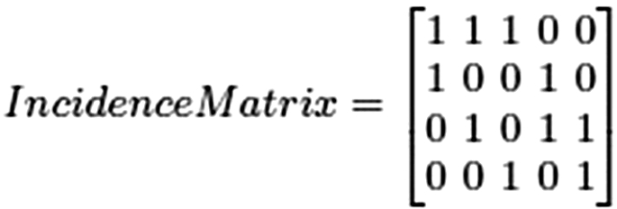
Incidence Matrix for the graph G in Fig. 1

A privileged reduced incidence edge structure (PRIES) of G is a table derived from RIES, such that the first column of the table contains edges incident on the reference vertex only, shown in Table 2. The reference vertex is a highest degree vertex of G. The columns are made compact so that each row represents the incident edges at the corresponding vertex in any order except the first column constraint.

Table 2 PRIES matrix generated by Sen Sarma’s algorithm for the graph G in Fig. 1

From PRIES all possible n − 1 edge combinations are generated by taking exactly one edge from each row and one edge from the first column while discarding combinations which are not distinct. These combinations have been shown in Table 3. These combinations are tested by the tree testing algorithm for distinguishing the tree sequences from the other non-tree sequences.

Table 3 Table showing edge combinations generated by Sen Sarma’s algorithm for the graph G in Fig. 1

The tree testing algorithm used by Sen Sarma exploits the property that every tree has at least two pendant vertices and any n − 1 edge combination cannot contain a cycle unless it has at least three nodes of degree more than one.

Authors did not provide any complexity analysis of Sen Sarma’s algorithm. So, we calculated the time and space complexity. There are three steps in the algorithm:

• 1. The first step is to generate PRIES matrix. In PRIES matrix, the maximum number of privileged column can be one and the maximum number of non-privileged columns can be (n − 1), as the highest degree of a vertex in G can be (n − 1). So, PRIES has a maximum 1 + (n − 1) = n number of columns and (n − 1) number of rows.

• 2. The second step is to generate edge combinations from PRIES. In each step, a new sequence of (n − 1) length is formed taking exactly one edge from each row while discarding sequences which are not distinct. Now, it is mandatory to take one element from the privileged column (i.e. the first column). So, combining these two, total n^n − 1 − (n − 1)ⁿ⁻¹ sequences can be generated.

• 3. The third step is to check whether each generated combination is a tree or not. We assume each combination checking takes T_c time.

Thus, the overall time required by this algorithm is approximately nⁿ × T_c. The term T_c is much less compared to nⁿ. Therefore, the overall time complexity is O(nⁿ). The space complexity of the algorithm is O(nm).

Naskar’s test and select algorithm

This algorithm [16] is an extension and improved version of Sen Sarma’s algorithm and was developed by Naskar et al. in 2007. The algorithm uses a super privileged reduced incidence edge structure (SPRIES).

Unlike Sen Sarma’s algorithm which uses only one privileged column, this algorithm has $\left\lfloor {2m/n} \right\rfloor$ number of privileged columns. The privileged columns are arranged in such a way that starting from the first column the highest degree vertices are chosen and the edges of the vertices are placed in the column only. Other elements of the row in PRIES are shifted right leaving the privileged columns free. Thus, SPRIES is generated by modifying PRIES.

From SPRIES, all possible n − 1 edge combinations are generated by taking exactly one edge from each row and one edge from the first column while discarding combinations which are not distinct. The combinations formed from only super privileged columns are spanning trees. The rest of the combinations are tested by the tree testing algorithm.

According to the authors, the time complexity of the algorithm is O(mn + n² + nτ(G)) and space required is O(mn).

Table 4 shows the SPRIES matrix generated from Table 2. The edge combinations generated by Naskar’s Test and Select algorithm have been shown in Table 5.

Table 4 SPRIES matrix generated by Naskar’s Test and Select algorithm from PRIES matrix in Table 2

Table 5 The table showing edge combinations generated by Naskar’s Test and Select algorithm for the graph G in Fig. 1

Onete’s algorithm

One of the most recent algorithms [19] for all spanning tree generation was proposed by Onete et al. in 2010. The algorithm uses a modified version of the incidence matrix of a graph to enumerate all the spanning trees.

The Incidence Matrix Inc of graph G is an (n × m) matrix, such that Inc_i,j = 1, if vertex v_i and edge e_j are incident, and 0, otherwise. Reduced Incidence Matrix RInc is obtained after removing the row of reference vertex from Inc, shown in Fig. 5. Any vertex from v₁ to v_n can be chosen as the reference vertex.

Fig. 5

Reduced Incidence Matrix for the graph G of Fig. 1, where Reference Vertex is v₄. So, the row corresponding to v₄ has been deleted

The Diagonal Matrix Diag is an (m × m) matrix with Diag_ij = e_i, where i = j, and Diag_ij = 0, where i ≠ j.

All spanning trees generation of graph G mainly depends upon the formation of matrix U (U = Diag × (RInc)^T), shown in Fig. 6. There is a one-to-one correspondence between ((n − 1) × (n − 1)) non-singular submatrices (determinant ≠ 0) of U and spanning trees. After formation of U, the algorithm follows a strictly top-down fashion considering an ((n − 1) × (n − 1)) non-singular submatrix in each iteration. If the matrix is permissible, i.e. contains at least a row of only one entry and the elements of the submatrix can be rearranged in such a manner that all diagonal elements are nonzero, then the entries on the diagonal indicates the spanning tree related to that particular nonsingular submatrix.

Fig. 6

U is the matrix product of Diagonal Matrix and Transpose of Reduced Incidence Matrix

The matrices generated by Onete’s algorithm for the graph G in Fig. 1 are shown in Fig. 7.

Fig. 7

Matrices related to edge combinations generated by Onete’s algorithm for the graph G in Fig. 1 are shown here

As the authors proposed, the time complexity of the algorithm is O(n + m + nτ(G)) and the space required is O(n + m).

Discussion on test and select algorithms

The test and select method generates (n − 1)-length edge combinations in the first phase and verifies each combination to be spanning tree or not in the second phase. So, tree testing is a mandatory part of this method.

The number of computations majorly depends on the number of sequences generated by an algorithm. Except Onete’s algorithm, the other three algorithms (Table 10) generate sequences containing duplicate edges. That means, no tracking of already visited edges has been used in these algorithms.

Generation of edge sequences can be made drastically faster if parallel execution approach is followed. Onete’s algorithm has the capacity to be implemented in this fashion.

In terms of number of sequences generated, the algorithms can be ranked as Char > Sen Sarma > Naskar > Onete. Thus, in Onete’s algorithm, least number of sequences is tested to be spanning trees. Some of the features of these algorithms have been described in Table 6.

Table 6 Comparison table of test and select algorithms

A close study of the above algorithms reveal that this test and select method should not be used for tree generation of a dense graph, which calls for more and more edge combinations to be formed. With an increase in the number of edge combinations, the number of non-trees generated is also supposed to increase proportionally. Consequently, the time taken to complete the whole process will be affected. Hence, we can conclude that the test and select method will be most suited for sparse graphs of moderate size and therefore this method is not recommended to be applied on social networking structures because even though the social network graphs are inherently sparse in nature but still the structure is massive and tree testing operation on such a huge structure will incur a massive computational cost. The other practical example of sparse graphs includes telecommunication networks where spanning tree generation finds several applications since the size of most of the telecommunication networks are much smaller compared to social network graphs; thus, the algorithms categorized under the test and select method can be utilized.

Trees by elementary tree transformation method

The algorithms classified under elementary tree transformation method create an initial spanning tree from the input graph G, generally by Breadth-First Traversal or Depth-First Traversal. So, the set of edges E is divided into two mutually exclusive subsets, Branch Set containing edges of the initial spanning tree and Chord Set containing edges which are not part of the initial spanning tree. Then at each step, a branch is replaced by a chord in such a way that no cycle is formed and all vertices remain connected. It is also known as cyclic interchange method. This is an optimized method in terms of generating only tree sequences. However, some logic has to be applied to avoid duplicate tree generation.

This method of generating spanning trees has been studied by several researchers [6, 10, 11, 13, 17, 21]. These algorithms have been discussed in the following sections.

Hakimi’s algorithm

The algorithm proposed by Hakimi [6] in 1961, generates all possible spanning trees of a graph in two phases. An initial tree t₀ = b₁, b₂, …, b_n−1 is formed, where b₁, b₂, …, b_n−1 are the branches of the graph G, shown in Fig. 8. The chord-set of t₀ be C = {c₁, c₂, …, c_N}, where N = m–n + 1. With respect to the above tree t₀, a fundamental circuit matrix is generated from where all trees of distance one from t₀ (represented by T₀₁) are derived by replacing each branch by each chord of each circuit. The fundamental circuit matrix is shown in Fig. 9 and T₀₁ is shown in Fig. 10. In the next phase, trees of distance two are found by considering all combinations of sets of trees of distance one. If T(c₁,c₂c₃ … c_N) be the set of trees with chord c₁ but without c₂, c₃, …, c_N and T(c₂,c₁c₃ … c_N) be the set of trees with chord c₂ but without c₁, c₃, …, c_N, the trees with both c₁ and c₂, represented by T(c₁c₂,c₃c₄ …c_N), can be derived from these two. This is continued until all trees of distance two, represented by T₀₂, are found out. Similarly, other trees at higher distances can also be found out using the above technique. The maximum distanced tree-set can be T_0N.

Fig. 8

Initial Tree (t₀ = e₁e₂e₃) obtained from Breadth First Traversal of the graph G of Fig. 1

Fig. 9

The fundamental circuit matrix (B_c) with respect to t₀, where Branch Set = {e₁, e₂, e₃} and Chord Set = {e₄, e₅}

Fig. 10

T₀₁ is the set of trees where either c₁ or c₂ is present

We have taken the input graph G in Fig. 1 and after BFS we have got t₀. All the trees of distance one from t₀ has to be generated first. From the circuit matrix in Fig. 9, we can write all trees of distance one from t₀ in matrix form by replacing each branch by each chord of each circuit. From T₀₁, we can find those trees T′(c₁, c₂) having only c₁ but not the other chord and T′(c₂, c₁) having only c₂ but not other chord, shown in Fig. 11.

Fig. 11

T′(c₁, c₂) and T′(c₂, c₁)

From T′(c₁, c₂) and T′(c₂, c₁), we can again find out those trees having both c₁ and c₂. Examination reveals that both have a common row. So, we form an intersection of the first row of T′(c₁, c₂) with two rows of T′(c₂, c₁) and of the second row of T′(c₂, c₁) with two rows of T′(c₁, c₂), shown in Fig. 12.

Fig. 12

T′_c1c2 is the set of trees having both the chords c₁ and c₂

The author did not derive any expression for time or space complexity of the algorithm. Hence, we derived them based on the given algorithm. The algorithm first finds out the fundamental circuit matrix of G. The number of fundamental circuits in a graph depends on the number of chords. Number of branches in G is (n − 1) and hence number of chords comes out to be (m − (n − 1)). Thus, computation of fundamental circuits requires at most O(m − n) time. Now from the circuit matrix, the trees at distance one from the initial tree are computed. This number is again dependent on the number of branches in each circuit, which is (n − 1). Thus the time involved in this computation is O(nm) for a dense graph. All the sequences generated may not be trees. The non-tree or duplicate sequences are discarded immediately. If we assume the number of trees generated is τ(G), then further computations, namely finding out the trees at higher distances from the initial tree, are dependent on τ(G). As a result, the overall worst case time complexity comes out to be O(nmτ(G)).

The fundamental circuit requires at most O(nm) space. The matrices storing the trees require O(mτ(G)) space. So, the overall space complexity is O(nm + mτ(G)), where τ(G) ≫ n, and hence, O(mτ(G)).

Mayeda’s algorithm

The algorithm developed by Mayeda et al. [13] in 1965, generates spanning trees by replacement of one branch by a group of selected chords one by one. The procedure starts with an initial tree and then computes the fundamental cut-sets of it. The initial spanning tree has been shown in Fig. 13. In a connected graph G = (V, E), a cut-set is a set of edges whose removal from G makes G disconnected, such that removal of no proper subset of these edges disconnects G. A cut-set containing exactly one branch of a given tree is called a fundamental cut-set with respect to the tree. The fundamental cut-set matrix for a given tree is obtained from the incidence matrix. Let S_e(t) be the fundamental cut-set with respect to branch e of tree t. Thus, S_e(t) contains e ∈ t but no other branch of t. All trees which are obtainable from a starting tree t₀ (also called the reference tree) by replacing branch e, can be obtained by replacing e with the chords in S_e(t₀) and these trees will be distinct. This set of trees has been denoted by T^e. That is,

Fig. 13

After Breadth First Traversal of G of Fig. 1, tree t₀ is generated

$$ T^{e} = \{ t|t = t_{0} \oplus \left\{ {e,e_{i} } \right\},e_{i} \in S_{e} \left( {t_{0} } \right),e_{i} \ne e\} $$

After that, an iterative procedure is applied which will replace another branch of t₀ in each of these sets. For a reference tree t₀ the class of trees T^{ei1ei2 … eik}, where (i₁, i₂, …, i_k) is a subset of (1, 2, …, e), which can be denoted by

$$ \begin{aligned} T^{ei1 \ldots eik} &= \bigg\{ t|t = t^{\prime } \oplus \left\{ {e_{ik} ,e_{j}^{\prime } } \right\},t^{\prime } \in T^{ei1 \ldots eik - 1} ,\\&\quad e_{i}^{\prime } \in S_{eik} \left( {t^{\prime } } \right) \cap S_{eik} \left( {t_{0} } \right),e_{ik} \ne e_{i}^{\prime } \bigg\} \end{aligned} $$

To avoid generation of duplicate trees, this algorithm orders the edges of initial tree as an M sequence. M sequence is a binary sequence generated by a deterministic algorithm. It is difficult to predict and exhibits statistical behavior similar to a truly random sequence.

The algorithm is hereby explained with the input graph G in Fig. 1. t₀ is the initial tree generated by Breadth-First Traversal of G.

According to the author, the time complexity of the algorithm is O(n + m + nmτ(G)) and the space required is O(n + m).

Kapoor’s algorithm

The algorithm was proposed by Kapoor et al. [10] in 1992. The algorithm generates an initial spanning tree T of G. Addition of one chord, e_k, where n ≤ k ≤ m, to T will result in formation of a fundamental cycle. Thus, a number of spanning trees can be generated from T by exchanging each branch of the fundamental cycle with the corresponding chord, e_k.

The computation can be represented by a computation tree with initial spanning tree T as root and the spanning trees generated by these exchanges as its children. Each child node is expanded recursively in the same manner as the root. Each recursive call generates a unique spanning tree of G. The algorithm maintains an inclusion set of edges, IN, and exclusion set of edges, OUT, at every node of the computation tree, in order to avoid generation of duplicate spanning trees. IN and OUT sets are empty for root node. For a node i in the computation tree, the set IN_i contains edges which are always a part of all the spanning trees at node i and its descendants. The set OUT_i contains edges which are not part of any spanning tree at node i or at its descendants.

The computation tree for Kapoor’s algorithm has been shown in Fig. 14.

Fig. 14

Computation Tree of Kapoor’s algorithm, for the graph G in Fig. 1. Each node is related to a state where a new edge combination has been generated, and sets IN and OUT get modified

Kapoor et al. mentioned that the time complexity of the algorithm is O(n + m + τ(G)) and the space required is O(mn).

Matsui’s algorithm

The algorithm was developed in 1993 by Matsui [11]. The algorithm starts with creating an initial spanning tree T by doing Breadth First Traversal or Depth First Traversal of the given input graph G. After that, edges are renumbered to create a linear ordering of edge-set such that branches are numbered as e₁, e₂, e₃, …, e_n − 1 and chords are numbered as e_n, e_n + 1, e_n + 2, …, e_m. Now, for each chord, it is checked whether the inclusion of that edge in the current spanning tree and the removal of a branch from the current spanning tree generates any cycle (or not). If not, then this replacement happens, and the newly generated spanning tree is called the child of the previous one. Algorithm terminates when no child of the previously generated spanning trees is possible.

A detailed description is given with an example to describe the approach of the algorithm. The input graph is G, shown in Fig. 1, and the set of edges is defined as E = {e₁, e₂, …, e_m}. We have performed Depth First Traversal to generate the initial spanning tree, shown in Fig. 15. In E, index of an edge e is described as Index(e). For any spanning tree T and for any edge f ∉ T, cycle (T, f) ⊆ E is a unique cycle in (V, T ∪ {f}). For any edge g ∈ T, the graph (V, T\{g}) contains two components. The set of edges in E connecting these two components becomes a cut-set denoted by cut (T, g). In an edge-subset E′ ⊆ E, the edge in E′ with the smallest index is top-edge of E′, i.e. top(E′). Edge in E′ with the largest index is the bottom-edge of E′, i.e. btm(E′).

Fig. 15

After Depth First Traversal of G in Fig. 1, tree T is generated. Branches are shown in thick lines and Chords are shown in dotted lines

The edge-subset T^* = {e₁, e₂, …, e_n−1} is the lexicographically minimum spanning tree of G. For any spanning tree T′ ≠ T^*, Ф(T′) indicates the spanning tree (T′\{f}) ∪ {g}, where f is the bottom-edge of T′ and g is the top-edge of the cut-set cut(T′, f). Let T be a spanning tree of G and T′ = (T\{g}) ∪ f is a child of T. g is the top-edge of cut (T′, f). Since, cut(T′, f) = cut(T, g), g is the top-edge of cut(T, g). Let, H(T) = {e′∈ T | e′ = top(cut(T, e′))}. Then, g ∈ H(T) and the edge f joins two different components of the graph (V, T\H(T)). Label ((V, T), H) returns the labels of two vertices in the graph. It says, two vertices will have the same level if and only if they are connected in the graph (V, T\H).

In Fig. 15, T = {e₁e₂e₃}, H = {e₁e₂e₃}, Chord Set = {e₄e₅}.

From Label ((V, T), H), we realize, all vertices have different labels. Index (btm(T)) = 3, so e₄ will be the first chord (f) to replace branches one by one.

$$ \begin{aligned} & D\, = \,cyc\left( {T,f} \right) \cap H = \left\{ {e_{ 1} e_{ 2} e_{ 3} } \right\}. \\ & {\text{When}}\;g\, = \,e_{ 1} ,\;{\text{then}}\;T_{ 1} = T\backslash \left\{ g \right\} \cup \left\{ f \right\} = T\backslash \left\{ {e_{ 1} } \right\} \cup \left\{ {e_{ 4} } \right\}\\ &\quad = \,\left\{ {e_{ 2} e_{ 3} e_{ 4} } \right\}. \\ & H_{ 1} = H\backslash \{ e\prime |Index(e\prime ) > Index\left( g \right)\} = H\backslash \left\{ {e_{ 2} e_{ 3} } \right\} = \left\{ {e_{ 1} } \right\}. \\ & {\text{Similarly}},\, {\text{when}}\, g \!=\! \left\{ {e_{ 2} } \right\},\, {\text{then}}\, T_{ 2} \!=\! \left\{ {e_{ 1} e_{ 3} e_{ 4} } \right\},\, H_{ 2} = \left\{ {e_{ 1} e_{ 2} } \right\}. \\ & {\text{When}}\;g = e_{ 3} ,\;{\text{then}}\;T_{ 3} = \left\{ {e_{ 1} e_{ 2} e_{ 4} } \right\},\;H_{ 3} = \left\{ {e_{ 1} e_{ 2} e_{ 3} } \right\}. \\ & {\text{Now}}\;f = e_{ 5} ,\;D = \left\{ {e_{ 1} e_{ 2} } \right\}. \\ & {\text{When}}\;g = e_{ 1} ,\;{\text{then}}\;T_{ 4} = \left\{ {e_{ 5} e_{ 2} e_{ 3} } \right\},\;H_{ 4} = \left\{ {e_{ 1} e_{ 3} } \right\}. \\ & {\text{When}}\;g = e_{ 2} ,\;{\text{then}}\;T_{ 5} = \left\{ {e_{ 1} e_{ 5} e_{ 3} } \right\},\;H_{ 5} = \left\{ {e_{ 1} e_{ 2} } \right\}. \\ \end{aligned} $$

T₁, T₂, T₃, T₄, and T₅ are children of T. Now children of already generated trees will be computed. T₁, T₂, T₄, and T₅ cannot have any children as they do not have any replaceable edge; Only T₃ can have children.

$$ \begin{aligned} &T_{ 3} = \left\{ {e_{ 1} e_{ 2} e_{ 4} } \right\},H_{ 3} = \left\{ {e_{ 1} e_{ 2} e_{ 3} } \right\}. \hfill \\ &f = e_{ 5} ,D = \left\{ {e_{ 1} e_{ 2} } \right\}. \hfill \\ &g = e_{ 1} ,T_{ 6} = \left\{ {e_{ 5} e_{ 2} e_{ 4} } \right\},H_{ 6} = \left\{ {e_{ 1} e_{ 3} } \right\}. \hfill \\ &g = e_{ 2} ,T_{ 7} = \left\{ {e_{ 1} e_{ 5} e_{ 4} } \right\},H_{ 7} = \left\{ {e_{ 1} e_{ 2} e_{ 3} } \right\}. \hfill \\ \end{aligned} $$

Now, T₆ and T₇ cannot have any child, so algorithm terminates here.

The time complexity of the algorithm is O(n + m+nτ(G)) and the space required is O(n + m), as mentioned by the author.

Shioura and Tamura’s algorithm

The algorithm was proposed by Shioura and Tamura [21] in 1993. The algorithm begins with the generation of a depth first spanning tree T⁰ of the input graph G. The smallest vertex v₁ is assumed to be the root of G. Each edge e_k ∈ G, where k = 1, 2, …, m has two incidence vertices, written as ∂⁺e_k and ∂⁻e_k, assuming that ∂⁺e_k ≤ ∂⁻e_k.

G is then relabeled such that the vertex-set V = {v₁, v₂, …, v_n} and edge-set E = {e₁, e₂, …, e_m} satisfy the following conditions:

• 1. T⁰ = {e₁, e₂, …, e_n−1}, any edge which belongs to T⁰ is smaller than any of its descendants.

• 2. Each vertex v which belongs to T⁰ is smaller than any of its descendants.

For any two edges e, f ∉ T⁰, e < f only if ∂⁺e ≤ ∂⁺f.

Let S be any non-empty subset of E. Let, Min(S) denotes the smallest edge in S, considering Min(Φ) = e_n. For any spanning tree T and any edge f ∈ T, the subgraph induced by the edge-set T\f has exactly two components. The set of edges connecting these components is called a fundamental cut associated with T and f, and represented as C^*(T\f). Thus, for any edge f ∈ T and for an arbitrary edge g ∈ C^*(T\f), T\f ∪ g is also a spanning tree. For any edge g ∉ T, the edge-induced subgraph of G by T ∪ g has a unique cycle, called a fundamental cycle associated with T and g. The set of edges of the cycle is represented as C(T ∪ g). For any g∉ T and for any f ∈ C(T ∪ g), T ∪ g\f is a spanning tree.

It is evident that, if f = Min(T⁰\T^c), then |C(T^c ∪ f) ∩ C^*(T⁰\f)\f | = 1 holds.

For any spanning tree T^p of G and for any two arbitrary edges f and g, let T^c= T^pf ∪ g. T^c be a child of T^p if and only if the following conditions hold:

• 1. e₁ ≤ f ≤ Min(T⁰\T^p), and

g ∈ C^* (T^p\f) ∩ C^* (T⁰\f)\f.

The algorithm outputs all children T^c of T^p not containing e_k and recursively calls itself for the following:

• 1. Generating all children of T^c (i.e. all grandchildren of T^p which do not contain e_k), and

• 2. Generating all children of T^p which contain e_k.

A detailed description is given with an example to describe the approach of the algorithm. We consider the same graph G = (V, E) as input, as shown in Fig. 1. A depth-first tree, T⁰ is obtained and the edges of the tree are relabeled in increasing order as they are visited. T⁰ is shown in Fig. 16. The relabeling is also done on G to match T⁰ and shown in Fig. 17. Thus, T⁰ = {1, 2, 3}.

Fig. 16

After Depth First Traversal of G in Fig. 1, tree T₀ is generated. Edges are renumbered in increasing order as they are visited

Fig. 17

The graph G after edge relabeling is performed, to match T⁰ in Fig. 16

Min(T⁰\T⁰) = Φ. So, edges 1, 2, 3 will be replaced one by one from T⁰.

Replacement of edge 1 is done as follows:

C^*(T⁰\1)\1 = {4, 5}. So, edges 4, 5 will replace edge 1 in T⁰, one at a time, to generate two spanning trees T⁰¹ and T⁰², respectively. Thus, T⁰¹ = {4, 2, 3} and T⁰² = {5, 2, 3}.

Similarly, replacing edge 2 from T⁰ will result in formation of T⁰³ = {1, 4, 3} and T⁰⁴ = {1, 5, 3}, and replacing edge 3 from T⁰ will result in formation of T⁰⁵ = {1, 2, 5}. This method is recursively followed for each of the new spanning trees, T⁰¹, T⁰², T⁰³, T⁰⁴, and T⁰⁵. The recursive calls will generate two more spanning trees from T⁰⁵, T⁵¹ = {4, 2, 5} and T⁵² = {1, 4, 5}. The computation is shown by the help of a computation tree in Fig. 18.

Fig. 18

Computation Tree of Shioura and Tamura’s algorithm where each node represents one spanning tree of graph G in Fig. 1

According to Shioura and Tamura, the time complexity of the algorithm is O(n + m+τ(G)) and space required is O(nm).

Naskar’s gray code algorithm

In 2009, Naskar et al. developed another all spanning tree generation algorithm [17] using Gray Codes. The algorithm creates an initial tree T of the input graph G by using Breadth-First Traversal, shown in Fig. 19. T contains n − 1 edges. So, there are n − 1 branches and m − (n − 1) chords. Then, binary representation of each number from 0 to 2 ^{m − (n − 1)} are generated, each of length m − (n − 1). These sequences are called Gray Codes. For each gray code, combination of n − 1 branches and m − (n − 1) chords will be computed in such manner that the output will contain n − 1 edges. Let a gray code sequence, g_i, contains k number of 1 s. So, k branches will be replaced by k chords in T. Each such combination, after cycle checking, is confirmed to be spanning tree or not. The combinations generated by the algorithm for the input graph G in Fig. 1 has been shown in Table 7.

Fig. 19

After Breadth First Traversal of G in Fig. 1, tree T is generated. Branch Set = {e₁, e₂, e₃} [{e_i, where e_i ∈ T}]; Chord Set = {e₄, e₅} [{e_i, where e_i ∉ T}]

Table 7 Table showing edge combinations generated by Naskar’s Gray Code algorithm for the graph G in Fig. 1

According to author, the time complexity of the algorithm is O(mlog(n) + n + τ(G)) and space required is O(n²).

Discussion on elementary tree transformation algorithms

The elementary tree transformation method initially creates one spanning tree and divides the edge set into two subsets—Branches and Chords. Then at each step, a new tree is generated by replacing one branch with a chord such that no cycle is introduced due to the replacement. So, cycle checking is here an essential part.

The main challenge of this method is to avoid generation of duplicate trees. Every algorithm under this category uses different approaches to generate distinct tree in each step. Kapoor’s algorithm [10] and Shioura’s algorithm [21] assure generation of a new spanning tree in each recursive call. As no non-tree sequence is generated, these two are the fastest algorithms in terms of time required to get executed. Table 8 shows the comparison of Elementary Tree Transformation Algorithms.

Table 8 Comparison table of elementary tree transformation algorithms

From Table 8 it is found that most of the tree transformation algorithms go for explicit cycle and/or cutset computation. This property can be utilized in many other problem areas where fundamental circuit and/or cutset computation is also required. Let us mention, in this regard, about one of the very well-known protocols used in networking, namely Spanning Tree Protocol (STP) that builds a loop-free logical topology for Ethernet networks by formation of spanning trees. It is used to provide fault tolerance in a network, by preventing bridge loops and the broadcast radiation that result from them. As a result, STP may significantly utilize the circuit computation feature of this class of algorithms. Similarly, cutset computation also plays a vital role in establishing network topologies. Besides, they also find huge applications in circuit theory and transportation networks.

Trees by successive reduction method

The concept of the successive reduction method is to divide a large graph into smaller subgraphs. The problem of spanning tree generation of the original graph is thus reduced to smaller problems of tree generation of the subgraphs. The division is continued till the reduced subgraphs are trivial like an edge. Spanning trees of the original graph are then obtained from the trees of the trivial subgraphs. This seems to be a little more complex method compared to the previously mentioned techniques. However, here it is always guaranteed that only distinct trees will be generated, also there is no need of performing any kind of tree testing. Some of the well-known algorithms [15, 25] falling under this classification are discussed in the next sections.

Minty’s algorithm

The algorithm was proposed by Minty [15] in 1965. The algorithm initiates by creating a partial spanning tree T containing all bridges of the input graph G = (V, E). An edge e_k is selected from G and the idea is to generate two classes of graphs G₁ and G₂, one containing e_k and another which does not contain e_k. G₁ is generated by shrinking e_k to a point and G₂ is generated by deletion of e_k, provided e_k is neither a self-loop nor a bridge. While generating G₁, the edge which is shrunk is added to T. G₁ and G₂ are reduced by deleting all self-loops and bridges. These bridges are added to T. This process is repeated until the graph is reduced to a single vertex. T generated at the end of each process is a spanning tree of G.

The algorithm has been described with the help of a computation tree in Fig. 20. The graph in Fig. 1 is the input. In the computation tree, +e_k denotes contraction of the edge e_k and − e_k denotes deletion of edge e_k.

Fig. 20

Computation tree of Minty’s algorithm

Minty did not provide any time or space complexity for the algorithm. Later, Smith [23] calculated the time and space complexity of the algorithm as O(n + m + mτ(G)) and O(n + m), respectively.

Winter’s algorithm

The algorithm developed by Winter [25] in 1986, performs consecutive contractions of the input graph, G. At first, the algorithm selects an edge e_k1 and constructs all the spanning trees containing e_k1, then it constructs all the spanning trees which include another edge e_k2 but not e_k1, and so on. The vertices and edges of G are relabeled as V = {1, 2, …, n} and E = {1, 2, …, m}. During each contraction, a vertex n_i is contracted into n_j, where n_i is the highest labeled vertex in the current graph and n_j is the highest labeled vertex adjacent to n_i.

The computation can be represented as a computation tree with the input graph G as the root. Each node in the computation tree has at most two children. The children of a node is obtained by either contracting an edge set S(n_i, n_j) or deleting the edge set S(n_i, n_j) followed by contraction of next S(n_i, n_j), where n_i and n_j are adjacent vertices in the parent graph. S(n_i, n_j) = {e_k | k = 1, 2, …, l}, where 1 ≤ l ≤ m, denote the edges between the vertex n_i and vertex n_j. Deletion of S(n_i, n_j) occurs only when n_i has adjacent vertices other than n_j. S(n_i, n_j) is contracted at each node until the graph gets reduced to a single vertex, labeled 1. The edges contracted at each step are stored in a sequence.

The algorithm is capable of examining more than one sequence simultaneously. This is possible because when a graph contracts, some edges may become parallel. There is no need to check for bridges. Moreover, the algorithm generates the sequence in such way that each sequence generates at least one of the spanning trees of G.

The algorithm has been described with the help of a computation tree, shown in Fig. 21, with the graph, G in Fig. 1, as input. The edges of the input graph, which have been contracted at each step, are written over the edges in the computation tree. Each node in the computation tree is denoted by G^X, where X is the set of vertices towards which the contraction took place in the previous step. The spanning trees are listed below the leaf nodes.

Fig. 21

Computation tree of Winter’s algorithm

Winter mentioned that the time complexity of the algorithm is O(n + m + min{nt, n!(n − 1)/2}) and the space required is O(n²).

Discussion on successive reduction algorithms

The method of successive reduction of a graph is based on systematic contraction and deletion of edges from the input graph to generate all spanning trees. Thus, the input graph reduces in size at each step either by contraction or by deletion of edge. The algorithm stops when the graph is reduced to a single vertex.

Contraction of edges may result in formation of parallel edges. Minty’s algorithm [15] contracts parallel edges one at a time and generates subtree sequences, whereas Winter’s algorithm contracts all the parallel edges in a single step and generates forest sequences. After the graph is reduced to a single vertex, Minty’s algorithm generates exactly one spanning tree and Winter’s algorithm [25] generates at least one spanning tree.

Deletion of an edge may result in formation of bridges. Minty’s algorithm checks for bridges after deletion of each edge. The bridges are then deleted and added to the subtree sequence. However, Winter’s algorithm does not perform any bridge checking. The algorithm contracts each bridge rather than deleting it. As deletion is already a part of the algorithm, the overhead of bridge checking can be avoided.

Thus, Winter’s algorithm follows a better approach than Minty’s algorithm. Some of the features of these two algorithms have been described in Table 9.

Table 9 Comparison table of successive reduction algorithms

An interesting observation about the successive reduction method is that there is no requirement of tree checking unlike other methods.

It is worth mentioning that the contraction and the removal operations, which play a vital role in this category of algorithms, can be carried out simultaneously, independent of each other. As a result, these algorithms can be efficiently executed in parallel, if multiple processors are available. Then the time taken will be optimized significantly. In social network analysis, spanning tree plays an important role in the identification of relationships among individuals or groups. Inherently, the social networks are sparse in nature, which means the actual number of links is relatively small compared to the maximum possible links. Therefore, in case of social network graphs, it is recommended to pick and choose an algorithm which has been categorized under the successive reduction of graph method to make use of the inherent parallel nature of the proposed algorithms. Moreover, if from a given graph we want to construct the spanning trees with or without a specific edge, then the contraction and removal procedure of successive reduction algorithms are most appropriate.

Experimental results

We have implemented the above-mentioned twelve algorithms in C language on an Intel Core i3 quad-core processor with clock speed 2.4 GHz, 6 GB RAM. For testing purpose, we have used twenty different non-isomorphic graph instances ranging from n = 10 to n = 40. These instances have been generated by an algorithm proposed by Chakraborty et al. [2].

Tables 10, 11, and 12 show the CPU time for various algorithms. In the tables, the ith instance of a graph with x vertices and y edges is denoted by I_i (x, y). Time taken by each of the algorithms is shown in dd–hh–mm–ss format, where dd, hh, mm, and ss stand for days, hours, minutes, and seconds required to execute the algorithms on the specific instances, respectively.

Table 10 Comparison table of test and select algorithms

Table 11 Comparison table of elementary tree transformation algorithms

Table 12 Comparison table of successive reduction algorithms

The observations for some specific instances are shown in the form of a stacked bar chart in Fig. 22, where CPU time is plotted along Y-axis and the algorithms along X-axis. Every color corresponds to an instance. There are five instances and in every bar, there are five colors signifying the CPU time taken to execute those five instances.

Fig. 22

Graphical representation of CPU time taken by various algorithms for some specific instances

Our contribution

In this article we have discussed about the three categories of spanning tree generation algorithms and implemented twelve of them for various non isomorphic graph instances. In most of the cases, we used the specific data structure given by authors, such as PRIES in Sen Sarma’s algorithm [20], SPRIES in Naskar’s algorithm [16], etc. In all the implementations, we have utilized adjacency matrix and edge list structure for representing the input graph and the spanning trees generated. In some cases, we have used the incidence matrix structure as well. The CPU times taken by the procedures align with the time complexities proposed by the authors. We have calculated the time and space complexities of the algorithms proposed by Hakimi [6] and Sen Sarma [20]. It is evident from Table 12 that Winter’s algorithm [25] is the fastest from implementation perspective, though we welcome future scholars to counter us. From theoretical aspect, algorithms by Kapoor [10] and Shioura [21] have optimum time complexity which is proportional to the total number of spanning trees generated.

The approach which we have followed to inspect different algorithms can be extended or modified in future. From comparison perspective, some experiments could have been done to scrutinize the algorithms in a better way. Such as, for a particular order and size, all non-isomorphic graphs could have been used as instances for executing all the algorithms. We have used an instance of maximum order forty (where the number of spanning trees generated is around 337 million). If this maximum order could be increased, we might have seen a new picture. So, there are many different viable approaches, unconquered, to analyze the existing algorithms from a different point of view, which we hope to be explored in near future.

Finally, we would like to highlight the fact that, even though we tried to provide guidance on selection of an algorithm from a specific class, the actual selection will depend largely on the following important aspects:

• The asymptotic running time of the selected algorithm.

• The size of the input.

• The configuration of the underlying platform where the algorithm will be implemented.

• The feasibility of quickly understanding and implementing an algorithm within a given time frame.

• The inherent nature of the problem which needs to be addressed by the generation of all possible spanning trees.

Conclusion

In this paper, we have attempted to refer and analyze most of the important/prime algorithms given by different academicians in the domain of all possible spanning tree generation of a simple, undirected, and connected graph. After analyzing the above-mentioned three classifications of algorithms, we have drawn some inferences regarding the suitability of an algorithmic technique in a particular scenario or circumstance. For example, test and select method is supposed to give better performance for sparse graphs rather than dense ones. Successive reduction of graphs is the most suited method if multiple processors are available, as they are inherently parallel in nature. There are some algorithms of other categories too which can also be executed in parallel. Another very important observation is that some algorithms serve dual purposes. For example, if we want effective enumeration of fundamental cycles or cutsets of a graph along with all spanning tree generation, we find that the elementary tree transformation algorithms are most suited. Again, if from a given graph we want to construct the spanning trees with or without a specific edge, then the successive reduction algorithms are to be selected.

It can be still said that scope of improvement is there in each category. A new algorithm may also be generated by combining the concepts of three categories. The approach of examining the input graph has not been tried much by researchers till date. Every algorithm so far, uses a generalized approach no matter what kind of input graph is given. However, depending upon the connectivity of vertices of the input graph, different approaches can be taken for better results. Thus, a lot of paths are yet to be visited, a lot of stones are yet to be turned. In future, researchers will certainly try to explore more and more in this area.

References

Berger I (1967) The enumeration of trees without duplication. IEEE Trans Circuit Theory 14:417–418
Chakraborty M, Chowdhury S, Chakraborty J, Mehera R, Pal RK (2017) Generation of non-isomorphic graphs of specific order, manuscript
Char JP (1968) Generation of trees, two-trees and storage of master forests. IEEE Trans Circuit Theory 15:128–138
Deo N (1979) Graph theory with applications to engineering and computer science. Prentice Hall of India Pvt, Ltd
Gabow HN, Myers EW (1978) Finding all spanning trees of directed and undirected graphs. SIAM J Comput 7:280–287. https://doi.org/10.1137/0207024
Hakimi SL (1961) On trees of a graph and their generation. J Franklin Inst 272(5):347–359
Jayakumar R, Thulasiraman K (1980) Analysis and study of a spanning tree enumeration algorithm, proceedings Springer-Verlag lecture notes in math. Comb Graph Theory 833:284–289
Jayakumar R, Thulasiraman K, Swamy MNS (1984) Complexity of computation of a spanning tree enumeration algorithm. IEEE Trans Circuits Syst 31(10):853–860
Jayakumar R, Thulasiraman K, Swamy MNS (1989) MOD-CHAR: an implementation of char’s spanning tree enumeration algorithm and its complexity analysis. IEEE Trans Circuits Syst 36(2):219–228
Kapoor S, Ramesh H (1995) Algorithms for enumerating all spanning trees of undirected and weighted graphs. SIAM J Comput 24(2):247–265. https://doi.org/10.1137/S009753979225030X
Matsui T (1993) An algorithm for finding all the spanning trees in undirected graphs, technical report: METR 93-08, Department of Mathematical Engineering and Information Physics, University of Tokyo, Tokyo, Japan, Vol. 16, pp. 237–252. https://pdfs.semanticscholar.org/1beb/a0744299732f1e5e4f05eb8055f4b549c663.pdf. Accessed 7 Aug 2018
Matsui T (1997) A flexible algorithm for generating all the spanning trees in undirected graphs. Algorithmica 18:530–543
Mayeda W, Seshu S (1965) Generation of trees without duplications. IEEE Trans Circuit Theory 12:181–185
McIlroy MD (1968) Generator of spanning trees, algorithm 354. Commun ACM 12:511
Minty GJ (1965) A simple algorithm for listing all the trees of a graph. IEEE Trans Circuit Theory 12:120
Naskar S, Basuli K, and Sen Sarma S (2007) Generation of all spanning trees of a simple, symmetric, connected graph, national seminar on optimization technique, Department of Applied Mathematics, University of Calcutta
Naskar S, Basuli K, and Sen Sarma S (2009) Generation of all spanning trees, social science research network. https://doi.org/10.2139/ssrn.1433035
Naskar S, Basuli K, and Sen Sarma S (2012) Generation of All Spanning Trees in the Limelight, Advances in Computer Science and Information Technology, Second International Conference, CCSIT 2012, Bangalore, India, 2012, Proceedings Part III published by Springer, vol. 86, pp. 188–192
Onete CE and Onete MCC (2010) Enumerating all the spanning trees in an un-oriented graph—a novel approach, XIth International Workshop on Symbolic and Numerical Methods, Modeling and Applications to Circuit Design (SM2ACD), http://ieeexplore.ieee.org/document/5672365/. Accessed 7 Aug 2018
Sen Sarma S, Rakshit A, Sen R, Choudhury A (1981) An efficient tree generation algorithm. J Inst Electr Telecommun Eng 27(3):105–109
Shioura A, Tamura A (1993) Efficiently scanning all spanning trees of an undirected graph, research report: B-270. Department of Information Sciences, Tokyo Institute of Technology, Japan
Shioura A, Tamura A, Uno T (1994) An optimal algorithm for scanning all spanning trees of undirected graphs. SIAM J Comput 26:678–693. https://doi.org/10.1137/S0097539794270881
Smith MJ (1997) generating spanning trees. MS Thesis, Department of Computer Science, University of Victoria, USA
Trent HM (1954) Note on the enumeration and listing of all possible trees in a connected linear graph. Proc Natl Acad Sci USA 40:1004
Winter P (1986) An algorithm for the enumeration of spanning trees. BIT Numer Math 26:44–62
Acknowledgements
We would like to thank Abhinandan Khan, Department of Computer Science and Engineering, University of Calcutta, for giving us valuable suggestions during the development of this article.
Author information
Authors and Affiliations
Corresponding author
Additional information
Publisher’s Note
Springer Nature remains neutral with regard to jurisdictional claims in published maps and institutional affiliations.
Rights and permissions
Open Access This article is distributed under the terms of the Creative Commons Attribution 4.0 International License (http://creativecommons.org/licenses/by/4.0/), which permits unrestricted use, distribution, and reproduction in any medium, provided you give appropriate credit to the original author(s) and the source, provide a link to the Creative Commons license, and indicate if changes were made.
About this article
Cite this article
Chakraborty, M., Chowdhury, S., Chakraborty, J. et al. Algorithms for generating all possible spanning trees of a simple undirected connected graph: an extensive review. Complex Intell. Syst. 5, 265–281 (2019). https://doi.org/10.1007/s40747-018-0079-7
Received:
Accepted:
Published:
Issue Date:
DOI: https://doi.org/10.1007/s40747-018-0079-7