The Gamma/Weibull Customer Lifetime Model

Abstract

This paper proposes a new customer lifetime model: the Gamma/Weibull distribution (G/W). Similar to the Pareto/NBD model, we propose a G/W/NBD model by combining the G/W distribution with a negative binomial distribution (NBD) and study its properties such as (i) the probability that a customer to be alive at a time point; (ii) the expectation and variance of the number of transactions for a customer during a fixed time period; (iii) the conditional expectation and conditional variance of the number of future transactions for a customer during a fixed time period. Several simulation studies are conducted to investigate the forecasting accuracy and flexibility of the proposed model. A CDNOW data set is analyzed by the proposed model.

Appendix: Derivation of Equations

• (1) Derivation of Eq. (2.3) It is easily shown from Eq. (2.2), Assumption (iii) and (iv) that the cdf of the G/W distribution is given by $F(\tau |b,s,\beta )=1- (\frac{\beta }{\beta +\tau ^{b}})^s$, which leads to the following probability density function:

  $$\begin{aligned} f(\tau |b,s,\beta )=\frac{\partial F(\tau |b,s,\beta )}{\partial \tau }=\frac{b \tau ^{b-1} s \beta ^{s}}{(\beta +\tau ^{b})^{s+1}},\ \ \tau >0, \end{aligned}$$

  where $b,~s,~\beta >0$.

• (2) Derivation of Eq. (3.4) The expectation of $\theta _{i}$ is given by

  $$\begin{aligned} \begin{array}{lll} E(\theta _{i}|\eta ,T_i) &{}=&{} T_{i} P(\tau _{i}>T_{i})+\tau _{i} P(0<\tau _{i}<T_{i})\\ &{}=&{} T_{i} (1-P(\tau _{i}>T_{i}))+\int _{0}^{T_{i}}\tau _{i}f(\tau _{i}|b,\eta )d\tau _{i}\\ &{}=&{} T_{i} e^{-\eta T_{i}^{b}}+\int _{0}^{T_{i}}\tau _{i}b \eta \tau _{i}^{b-1} e^{-\eta \tau _{i}^{b}} \mathrm{d}\tau _{i}. \end{array} \end{aligned}$$

  (6.1)

  It is easily shown that

  $$\begin{aligned} \int _{0}^{T_{i}}\tau _{i}b \eta \tau _{i}^{b-1} e^{-\eta \tau _{i}^{b}} d\tau _{i}= -\frac{b T_{i}\mathrm{exp}(-\frac{1}{2}\eta T_{i}^b) M_{-\frac{1}{2b}, \frac{1}{2b}+\frac{1}{2}}(-\eta T_{i}^b)}{(b+1)(-\eta T_{i}^b)^{\frac{1}{2b}}}. \end{aligned}$$

  Combining above equations yields Eq. (3.4).

• (3) The aggregate-level likelihood The aggregate-level likelihood is given by

  $$\begin{aligned}&L(r,\alpha ,b,s,\beta |x_{i}, t_{x_{i}}, T_{i})\\&\quad = \int _{0}^{\infty } \int _{0}^{\infty } L(\lambda ,b,\eta |x_{i}, t_{x_{i}}, T_{i})f(\lambda |r,\alpha )f(\eta |s,\beta )\mathrm{d}\lambda \mathrm{d}\eta \\&\quad = \int _{0}^{\infty } \int _{0}^{\infty } \left[ \lambda ^{x_{i}} e^{-\lambda T_{i}} e^{-\eta T_{i}^{b}}+b\eta \lambda ^{x_{i}} \int _{t_{x_{i}}}^{T_{i}} e^{-\lambda \tau _{i}} \tau _{i}^{b-1} e^{-\eta \tau _{i}^{b}}\mathrm{d}\tau _{i} \right] \\&\qquad \times f(\lambda |r,\alpha )f(\eta |s,\beta )\mathrm{d}\lambda \mathrm{d}\eta \\&\quad = I_{1}+I_{2}, \end{aligned}$$

  where

  $$\begin{aligned} I_{1}= & {} \int _{0}^{\infty } \int _{0}^{\infty } \lambda ^{x_{i}} e^{-\lambda T_{i}} e^{-\eta T_{i}^{b}} \frac{\alpha ^{r}}{\varGamma (r)} \lambda ^{r-1} e^{-\lambda \alpha } \frac{\beta ^{s}}{\varGamma (s)} \eta ^{s-1} e^{-\eta \beta }\mathrm{d}\lambda \mathrm{d}\eta \\= & {} \int _{0}^{\infty } e^{-\eta T_{i}^{b}} \frac{\beta ^{s}}{\varGamma (s)} \eta ^{s-1} e^{-\eta \beta } \int _{0}^{\infty } \lambda ^{x_{i}} e^{-\lambda T_{i}} \frac{\alpha ^{r}}{\varGamma (r)} \lambda ^{r-1} e^{-\lambda \alpha } \mathrm{d}\lambda \mathrm{d}\eta \\= & {} \frac{\varGamma (x_{i}+r)}{\varGamma (r)}\left( \frac{\alpha }{\alpha +T_{i}}\right) ^{r} \left( \frac{1}{\alpha +T_{i}}\right) ^{x_{i}} \left( \frac{\beta }{\beta +T_{i}^{b}}\right) ^s. \\ I_{2}= & {} \int _{t_{x_{i}}}^{T_{i}} b \tau _{i}^{b-1} \int _{0}^{\infty } \eta e^{-\eta \tau _{i}^{b}} \frac{\beta ^{s}}{\varGamma (s)} \eta ^{s-1} e^{-\eta \beta } \int _{0}^{\infty } \lambda ^{x_{i}} e^{-\eta \tau _{i}^{b}} \frac{\alpha ^{r}}{\varGamma (r)} \lambda ^{r-1} e^{-\lambda \alpha } \mathrm{d}\lambda \mathrm{d}\eta \mathrm{d}\tau _{i}\\= & {} \frac{bs\alpha ^{r} \beta ^{s} \varGamma (x_{i}+r)}{\varGamma (r)} \int _{t_{x_{i}}}^{T_{i}} \tau _{i}^{b-1} (\tau _{i}+\alpha )^{-(x_{i}+r)} (\beta +\tau _{i}^{b})^{-(s+1)} \mathrm{d}\tau _{i}. \end{aligned}$$

  Combining the above equations leads to Eq. (3.12).

• (4) Derivation of Eq. (3.13)

  $$\begin{aligned}&P(X_{i}=x_{i}|r,\alpha ,b,s,\beta ,T_{i})\\&\quad =\int _{0}^{\infty } \int _{0}^{\infty } P(X_{i}=x_{i}|\lambda ,b,\eta ,T_{i})f(\lambda |r,\alpha )f(\eta |s,\beta ) \mathrm{d}\lambda \mathrm{d}\eta \\&\quad =\int _{0}^{\infty } \int _{0}^{\infty } \frac{(\lambda T_{i})^{x_{i}} e^{-\lambda T_{i}}}{x_{i}!} e^{-\eta T_{i}^{b}}f(\lambda |r,\alpha )f(\eta |s,\beta ) \mathrm{d}\lambda \mathrm{d}\eta \\&\qquad +\int _{0}^{\infty } \int _{0}^{\infty } \int _{0}^{T_{i}}\frac{(\lambda \tau _{i})^{x_{i}} e^{-\lambda \tau _{i}}}{x_{i}!} b \eta \tau _{i}^{b-1} e^{-\eta \tau _{i}^{b}} \mathrm{d}\tau _{i} f(\lambda |r,\alpha )f(\eta |s,\beta ) \mathrm{d}\lambda \mathrm{d}\eta \\&\quad = I_{3}+I_{4}, \end{aligned}$$

  where

  $$\begin{aligned} I_{3}= & {} \frac{T_{i}^{x_{i}}}{x_{i}!}\int _{0}^{\infty } e^{-\eta T_{i}^{b}}f(\eta |s,\beta ) \int _{0}^{\infty } \lambda ^{x_{i}} e^{-\lambda T_{i}} \frac{\alpha ^{r}}{\varGamma (r)} \lambda ^{r-1} e^{-\lambda \alpha } \mathrm{d}\lambda \mathrm{d}\eta \\= & {} \frac{1}{x_{i}!}\frac{\varGamma (x_{i}+r)}{\varGamma (r)}\Bigg (\frac{\alpha }{\alpha +T_{i}}\Bigg )^{r} \Bigg (\frac{T_{i}}{\alpha +T_{i}}\Bigg )^{x_{i}} \Bigg (\frac{\beta }{\beta +T_{i}^{b}}\Bigg )^{s},\\ I_{4}= & {} \frac{1}{x_{i}!} \int _{0}^{T_{i}} b \tau _{i}^{x_{i}+b-1} \int _{0}^{\infty } \eta e^{-\eta \tau _{i}^{b}} \frac{\beta ^{s}}{\varGamma (s)} \eta ^{s-1} e^{-\eta \beta } \int _{0}^{\infty } \lambda ^{x_{i}} e^{-\lambda \tau _{i}} \frac{\alpha ^{r}}{\varGamma (r)} \lambda ^{r-1} e^{-\lambda \alpha } \mathrm{d}\lambda \mathrm{d}\eta \mathrm{d}\tau _{i}\\= & {} \frac{\alpha ^{r}}{x_{i}!} \frac{\varGamma (x_{i}+r)}{\varGamma (r)} \int _{0}^{T_{i}} b \tau _{i}^{x_{i}+b-1} (\tau _{i}+\alpha )^{-(x_{i}+r)} \int _{0}^{\infty } \eta e^{-\eta \tau _{i}^{b}} \frac{\beta ^{s}}{\varGamma (s)} \eta ^{s-1} e^{-\eta \beta } \mathrm{d}\eta \mathrm{d}\tau _{i}\\= & {} \frac{\alpha ^{r} b s \beta ^{s}}{x_{i}!} \frac{\varGamma (x_{i}+r)}{\varGamma (r)} \int _{0}^{T_{i}} \tau _{i}^{x_{i}+b-1} (\tau _{i}+\alpha )^{-(x_{i}+r)} (\beta +\tau _{i}^{b})^{-(s+1)} \mathrm{d}\tau _{i}, \end{aligned}$$

  Combining the above equations yields Eq. (3.13).

• (5) Derivation of Eq. (3.15) Similar to (A.1), the mth order moment of $\theta _i$ at zero of the lifetime distribution for customer i can be expressed as $E(\theta _{i}^m|\eta ,T_i)=T_{i}^m e^{-\eta T_{i}^{b}}+\int _{0}^{T_{i}}\tau _{i}^m b \eta \tau _{i}^{b-1} e^{-\eta \tau _{i}^{b}} d\tau _{i}$. Then, the mth order moment of $\theta _i$ at zero of the lifetime distribution for a randomly picked customer i over the interval $(0, T_i]$ is given by

  $$\begin{aligned} E(\theta _{i}^m|b,s,\beta ,T_i)= & {} \int _{0}^{\infty } (T_{i}^m e^{-\eta T_{i}^{b}}+\int _{0}^{T_{i}}\tau _{i}^m b \eta \tau _{i}^{b-1} e^{-\eta \tau _{i}^{b}})f(\eta |s,\beta ) \mathrm{d}\tau _{i} \mathrm{d}\eta \\= & {} T_{i}^m \int _{0}^{\infty } e^{-\eta T_{i}^{b}} f(\eta |s,\beta ) \mathrm{d}\eta \\&+ \int _{0}^{T_{i}} b \tau _{i}^{m+b-1} \int _{0}^{\infty } \eta e^{-\eta \tau _{i}^{b}}f(\eta |s,\beta ) \mathrm{d}\eta \mathrm{d}\tau _{i}\\= & {} \left( \frac{\beta }{\beta +T_{i}^b}\right) ^s T_{i}^m + bs\beta ^{s}\int _{0}^{T_{i}} \tau _{i}^{m+b-1} (\beta +\tau _{i}^b)^{-(s+1)}\mathrm{d}\tau _{i}. \end{aligned}$$

• (6) Derivation of Eq. (3.17) It is easily shown from Assumption (iv) that a randomly picked customer i who is still alive at $T_{i}$ has a death process proceeding from $T_{i}$ that follows a G/W distribution with the updated parameters $s^{*}=s$ and $\beta ^{*}=\beta +T_{i}^{b}$. Again, because the purchase made by a randomly picked customer i in $(T_{i}, T_{i}+T^{*}]$ follows the NBD model with parameters $r^{*}=r+x_{i}$ and $\alpha ^{*}=\alpha +T_{i}$, the conditional expectation of the number of future transactions while alive at $T_{i}$ is given by

  $$\begin{aligned}&E(x_{i}^\star |r^\star ,\alpha ^\star ,b,s^\star ,\beta ^\star , \mathrm{~alive~at~} T_{i})\\&\quad =\int _{0}^{\infty } \int _{0}^{\infty } E(x_{i}^\star |\lambda ,b,\eta , \mathrm{~alive~at~} T_{i})f(\lambda |r^\star ,\alpha ^\star ) f(\eta |s^\star ,\beta ^\star ) \mathrm{d}\lambda \mathrm{d}\eta \\&\quad = \int _{0}^{\infty } \int _{0}^{\infty } \{\lambda T^\star \mathrm{exp}(-\eta [(T_{i}+T^\star )^{b}-T_{i}^{b}]) \\&\quad \quad +\, \lambda \int _{0}^{T^\star } \tau _{i}f(\tau _{i}|b,\eta ,\tau _{i}>0)d\tau _{i} \}f(\lambda |r^\star , \alpha ^\star )f(\eta |s^\star ,\beta ^\star ) \mathrm{d}\lambda \mathrm{d}\eta \\&\quad = \frac{r^\star }{\alpha ^\star } \int _{0}^{\infty } \{ T^\star \mathrm{exp}(-\eta [(T_{i}+T^\star )^{b}-T_{i}^{b}])\\&\quad \quad + \int _{0}^{T^\star } \tau _{i}f(\tau _{i}|b,\eta ,\tau _{i}>0)d\tau _{i} \}f(\eta |s^\star ,\beta ^\star )\mathrm{d}\eta \\&\quad = \frac{r^\star }{\alpha ^\star } (I_{5}+I_{6}). \end{aligned}$$

  It is easily shown that

  $$\begin{aligned} I_5=\left( \frac{\beta ^\star }{\beta ^\star +(T_{i}+T^\star )^{b}-T_{i}^{b}}\right) ^s T^\star ,\ \ I_6=bs\beta ^{\star s} \int _{0}^{T^\star } \tau _{i}^{b} (\beta ^\star +\tau _{i}^{b})^{-(s+1)}\mathrm{d}\tau _{i}. \end{aligned}$$

  Combining the above equations leads to Eq. (3.17).

• (7) Derivation of Eq. (3.19) It follows from Eq. (3.6) that

  $$\begin{aligned}&E(x_{i}^{\star 2}|r^\star ,\alpha ^\star ,b,s^\star ,\beta ^\star , \mathrm{~alive~at~} T_{i})\\&\quad =\int _{0}^{\infty } \int _{0}^{\infty } E(x_{i}^{\star 2}|\lambda ,b,\eta ,\mathrm{~alive~at~} T_{i}) f(\lambda |r^\star ,\alpha ^\star )f(\eta |s^\star ,\beta ^\star ) \mathrm{d}\lambda \mathrm{d}\eta \\&\quad = \int _{0}^{\infty } \int _{0}^{\infty } \{ [\lambda T^\star +(\lambda T^\star )^{2}] P(\tau _{i}>T_{i}+T^\star |b,\eta ,\tau _{i}>T_{i})\\&\qquad + \int _{0}^{T^\star } [\lambda \tau _{i}+(\lambda \tau _{i})^{2}] f(\tau _{i}|b,\eta ,\tau _{i}>0)\mathrm{d}\tau _{i} \}f(\lambda |r^\star ,\alpha ^\star )f(\eta |s^\star ,\beta ^\star ) \mathrm{d}\lambda \mathrm{d}\eta \\&\quad = \int _{0}^{\infty } \int _{0}^{\infty } E(x_{i}^\star |\lambda ,b,\eta ,\mathrm{~alive~at~} T_{i}) f(\lambda |r^\star ,\alpha ^\star )f(\eta |s^\star ,\beta ^\star ) \mathrm{d}\lambda \mathrm{d}\eta \\&\qquad + \int _{0}^{\infty } \int _{0}^{\infty } (\lambda T^\star )^{2} \mathrm{exp}(-\eta [(T_{i}+T^\star )^{b}-T_{i}^{b}]) f(\lambda |r^\star ,\alpha ^\star )f(\eta |s^\star ,\beta ^\star ) \mathrm{d}\lambda \mathrm{d}\eta \\&\qquad + \int _{0}^{\infty } \int _{0}^{\infty } \lambda ^{2} \int _{0}^{T^\star }\tau _{i}^{2}f(\tau _{i}|b,\eta ,\tau _{i}>0)d\tau _{i} f(\lambda |r^\star ,\alpha ^\star )f(\eta |s^\star ,\beta ^\star ) \mathrm{d}\lambda \mathrm{d}\eta \\&\quad = I_{7}+I_{8}+I_{9}. \end{aligned}$$

  It is easily shown from Eq. (3.17) that $I_{7}=E(x_{i}^\star |r^\star ,\alpha ^\star ,b,s^\star ,\beta ^\star ,\mathrm{alive~at~}T_{i})$, $I_8=\{r^\star /\alpha ^{\star 2}+(r^\star /\alpha ^\star )^2\}[\beta ^\star /\{\beta ^\star + (T_{i}+T^\star )^{b}-T_{i}^{b}\}]^{s} T^{\star 2}$, and $I_9=\{r^\star /\alpha ^{\star 2}+(r^\star /\alpha ^\star )^2\} b s \beta ^{\star s} \int _{0}^{T^\star } \tau _{i}^{b+1} (\beta ^\star +\tau _{i}^{b})^{-(s+1)}\mathrm{d}\tau _{i}$. Combining the above equations yields Eq. (3.19).

• (8) The conditional expectation and variance of the number of future transactions for a randomly picked customer i with purchasing history $(x_{i}, t_{x_{i}}, T_{i})$ over the period $(T_i,T_{i}+T^\star ]$. We first prove that the Gompertz distribution lacks of memoryless property. For any $t,T>0$, if a random variable $\tau$ follows the Gompertz distribution with scale parameter b and shape parameter $\eta$, we have

  $$\begin{aligned} \begin{array}{lll} P(\tau>T+t|b,\eta ,\tau>T) &{}=&{} \frac{P(\tau>T+t, \tau>T)}{P(\tau >T)}=\frac{1-P(\tau \le T+t)}{1-P(\tau \le T)}\\ &{}=&{} \frac{\exp \{-\eta (e^{b(T+t)}-1)\}}{\exp \{-\eta (e^{bT}-1)\}} = e^{-\eta e^{bT}(e^{bt}-1)}. \end{array} \end{aligned}$$

  (6.2)

  Because $e^{-\eta e^{bT}(e^{bt}-1)} \ne e^{-\eta (e^{bt}-1)}$, the Gompertz distribution lacks of memoryless property. Thus, we have

  $$\begin{aligned} P(\tau _{i}>T_{i}+T^{*}|b,\eta ,\tau _{i}>T_{i})=\exp \{-\eta e^{b T}(e^{b T^\star }-1)\}. \end{aligned}$$

  (6.3)

  It is easily shown from the assumption given in Bemmaor and Glady [3] that a randomly picked customer i who is still alive at $T_{i}$ has a death process proceeding from $T_{i}$ that follows a G/G distribution with the updated parameters $s^{*}=s$ and $\beta ^{*}=\beta +e^{b T_{i}}-1$. Similarly, the purchase made by a randomly picked customer i in $(T_{i}, T_{i}+T^{*}]$ follows the NBD model with parameters $r^{*}=r+x_{i}$ and $\alpha ^{*}=\alpha +T_{i}$. For a randomly picked customer i with purchase history $(x_{i}, t_{x_{i}}, T_{i})$, the conditional expectation of the number of future transactions $x_{i}^{*}$ over the period $(T_{i}, T_{i}+T^{*}]$ is given by $E(x_{i}^{*}|r,\alpha ,b,s,\beta ,x_i, t_{x_{i}},T_{i}, T^{*})=E(x_{i}^\star |r^\star ,\alpha ^\star ,b,s^\star$, $\beta ^\star , \mathrm{alive~at~}T_{i}) P(\tau _{i}>T_{i}|r,\alpha ,b,s,\beta ,x_i, t_{x_{i}},T_{i})$, where $P(\tau _{i}>T_{i}|r,\alpha , b,s,\beta ,x_{i}$, $t_{x_{i}}, T_{i})$ is given in Eq. (29) of Bemmaor and Glady [3]. Now we derive $E(x_{i}^\star |r^\star , \alpha ^\star , b,s,\beta ^\star ,\mathrm{alive~at~}T_{i})$. From Eqs. (3.9), (6.3) and the pdf of the Gompertz distribution, we obtain

  

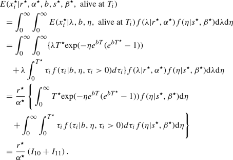
  It is easily shown that $I_{10}=[\beta ^\star /\{\beta ^\star +e^{b T}(e^{b T^\star }-1)\}]^{s} T^\star$ and $I_{11}=bs\beta ^{\star s} \int _{0}^{T^\star } \tau _{i}$$e^{b\tau _{i}} (\beta ^\star +e^{b\tau _{i}}-1)^{-(s+1)}\mathrm{d}\tau _{i}$. Combining the above equations leads to $E(x_{i}^\star |r^\star ,\alpha ^\star$, $b,s^\star ,\beta ^\star , \mathrm{~alive~at~} T_{i})$. For a randomly picked customer i with purchase history $(x_{i}, t_{x_{i}}, T_{i})$, the conditional variance of the number of future transactions $x_{i}^{*}$ over the period $(T_{i}, T_{i}+T^{*}]$ is given by $\mathrm{var}(x_{i}^{*}|r,\alpha ,b,s,\beta ,x_i, t_{x_{i}},T_{i}, T^{*})=E(x_{i}^{*2}|r,\alpha ,b,s,\beta ,x_i$, $t_{x_{i}},T_{i}, T^{*}) -[E(x_{i}^{*}|r,\alpha ,b,s,\beta ,x_i, t_{x_{i}},T_{i}, T^{*})]^{2}.$ Note that $E(x_{i}^{*2}|r,\alpha ,b,s,\beta ,x_i$, $t_{x_{i}},T_{i}, T^{*})=E(x_{i}^{*2}|r^{*},\alpha ^{*},b,s^{*},\beta ^{*},\mathrm{alive~at~}T_{i})P(\tau _{i}>T_{i}|r,\alpha ,b,s,\beta ,x_i, t_{x_{i}},T_{i})$, where $P(\tau _{i}>T_{i}|r,\alpha , b,s,\beta ,x_{i}, t_{x_{i}}, T_{i})$ is given in (29) of Bemmaor and Glady [3]. By Eqs. (3.9), (6.3) and the pdf of the Gompertz distribution, we obtain

  $$\begin{aligned} \begin{array}{lll} E(x_{i}^{\star 2}|r^\star ,\alpha ^\star ,b,s^\star ,\beta ^\star ,\mathrm{alive~at~}T_{i}) &{}=&{} E(x_{i}|r^\star ,\alpha ^\star ,b,s^\star ,\beta ^\star ,\mathrm{alive~at~}T_{i})\\ &{}&{}+\left[ \frac{r^\star }{\alpha ^{\star 2}}+\left( \frac{r^\star }{\alpha ^\star }\right) ^{2}\right] \left\{ \left( \frac{\beta ^\star }{\beta ^\star +e^{b T}(e^{b T^\star }-1)}\right) ^{s} T^{\star 2}\right. \\ &{}&{}\left. +bs\beta ^{\star s} \int _{0}^{T^\star } \tau _{i}^{2} e^{b\tau _{i}} (\beta ^\star +e^{b\tau _{i}}-1)^{-(s+1)}\right\} .\\ \end{array} \end{aligned}$$

References

Schmittlein, D.C., Morrison, D.G., Colombo, R.: Counting your customers: Who are they and what will they do next? Manag. Sci. 33(1), 1–24 (1987)
Fader, P.S., Hardie, B.G.S., Lee, K.L.: Counting your customers the easy way: an alternative to the Pareto/NBD model. Mark. Sci. 24(2), 275–284 (2005a)
Bemmaor, A.C., Glady, N.: Modeling purchasing behavior with sudden death: a flexible customer lifetime model. Manag. Sci. 58(5), 1012–1021 (2012)
Reinartz, W.J., Kumar, V.: On the profitability of long-life customer in a noncontractual setting: an empirical investigation and implications for marketing. J. Mark. 64(4), 17–35 (2000)
Jain, D., Singh, S.S.: Customer lifetime value research in marketing: a review and future directions. J. Interact. Mark. 16, 34–46 (2002)
Reinartz, W.J., Kumar, V.: The impact of customer relationship characteristics on profitable lifetime duration. J. Mark. 67(1), 77–99 (2003)
Ho, T.-H., Park, Y.-H., Zhou, Y.-P.: Incorporating satisfaction in to customer value analysis: optimal investment in lifetime value. Mark. Sci. 25(3), 260–277 (2006)
Jerath, K., Fader, P.S., Hardie, B.G.S.: New perspectives on customer death using a generalization of the Pareto/NBD model. Mark. Sci. 30(5), 866–880 (2011)
Makoto, A.: Counting your customers one by one: a hierarchical Bayes extension to the Pareto/NBD model. Mark. Sci. 28(3), 541–553 (2009)
Jardine, A.K.S., Anderson, P.M., Mann, D.S.: Application of the Weibull proportional hazards model to aircraft and marine engine failure date. Qual. Reliab. Eng. Int. 3, 77–82 (1987)
Odell, P.M., Anderson, K.M., D’Agostino, R.B.: Maximum likelihood estimation for interval-censored data using a Weibull-based accelerated failure time model. Biometrics 48(3), 951–959 (1992)
Sewalem, A., G. J. Kistemaker, F. Miglior, B. J. Van Doormaal.: Analysis of the relationship between type traits and functional survival in canadian holstein using a Weibull proportional hazard model. J. Dairy Sci. 87, 3938–3946 (2004)
Casellas, J.: Bayesian inference in a piecewise Weibull proportional hazards model with unknown change points. J. Anim. Breed. Genet. 124, 176–184 (2007)
Carrasco, J.M.F., Ortega, E.M.M., Cordeiro, G.M.: A generalized modified Weibull distribution for lifetime modeling. Comput. Stat. Data Anal. 53, 450–462 (2008)
Zhang, Q., Hua, C., Xu, G.: A mixture Weibull proportional hazard model for mechanical system failure prediction utilising lifetime and monitoring data. Mech. Syst. Signal Process. 43, 103–112 (2014)
Almalki, S.J., Nadarajah, S.: Modifications of the Weibull distribution: a review. Reliab. Eng. Syst. Saf. 124, 32–55 (2014)
Sha, N., Pan, R.: Bayesian analysis for step-stress accelerated life testing using Weibull proportional hazard model. Stat Papers 55, 715–726 (2014)
Kern, E.L., Cobuci, J.A., Costa, C.N., Ducrocq, V.: Survival analysis of productive life in Brazilian holstein using a piecewise Weibull proportional hazard model. Livest. Sci. 185, 89–96 (2016)
Ehrenberg, A.S.C.: Repeat Buying, North-Holland, Amsterdam (1972)
Morrison, D.G.: Analysis of consumer purchase data: a Bayesian approach. Ind. Manag. Rev. 9, 31–40 (1968)
Fader, P.S., Hardie, B.G.S.: Forecasting repeat sales at CDNOW: a case study. Part 2 of 2. Interfaces 31, S94–S107 (2001)
Fader, P.S., Hardie, B.G.S., Lee, K.L.: RFM and CLV: using iso-value curves for customer base analysis. J. Mark. Res. 42(4), 415–430 (2005b)
Acknowledgements
The authors are grateful to the Editor, an Associate Editor and a referee for their valuable suggestions and comments for largely improving the manuscript. The research was supported by grants from the National Natural Science Foundation of China (Grant No.: 11165016) and Key Projects of the National Natural Science Foundation of China (Grant No.: 11731101).
Author information
Authors and Affiliations
Corresponding author