
Abstract
In this paper, we present a new connection between representation theory of noncommutative hypersurfaces and combinatorics. Let S be a graded (\(\pm 1\))-skew polynomial algebra in n variables of degree 1 and \(f =x_1^2 + \cdots +x_n^2 \in S\). We prove that the stable category \(\mathsf {\underline{CM}}^{\mathbb Z}(S/(f))\) of graded maximal Cohen–Macaulay module over S/(f) can be completely computed using the four graphical operations. As a consequence, \(\mathsf {\underline{CM}}^{\mathbb Z}(S/(f))\) is equivalent to the derived category \(\mathsf {D}^{\mathsf {b}}({\mathsf {mod}}\,k^{2^r})\), and this r is obtained as the nullity of a certain matrix over \({\mathbb F}_2\). Using the properties of Stanley–Reisner ideals, we also show that the number of irreducible components of the point scheme of S that are isomorphic to \({\mathbb P}^1\) is less than or equal to \(\left( {\begin{array}{c}r+1\\ 2\end{array}}\right) \).
1 Introduction
Triangulated categories play an increasingly important role in many areas of mathematics, including representation theory, (commutative and noncommutative) algebraic geometry, algebraic topology, and mathematical physics. In particular, there are two major classes of triangulated categories, namely, the (bounded) derived categories \(\textsf {D}^\textsf {b}({\textsf {A}})\) of abelian categories \({\textsf {A}}\) and the stable categories \({\underline{{\textsf {C}}}}\) of Frobenius categories \({\textsf {C}}\). For example, the derived categories \({\textsf {D}}^{\textsf {b}}({\textsf {coh}}\,X)\) of coherent sheaves on algebraic varieties X have been studied extensively in algebraic geometry, and the stable categories  of maximal Cohen–Macaulay modules over (not necessary commutative) Gorenstein algebras A have been studied extensively in representation theory of algebras. In this paper, we compute the stable categories
  of graded maximal Cohen–Macaulay modules over certain noncommutative quadric hypersurface rings A (in the sense of Smith and Van den Bergh [7]) using combinatorial methods.
Throughout let k be an algebraically closed field of characteristic not 2. It is well-known that if A is the homogeneous coordinate ring of a smooth quadric hypersurface in \(\mathbb {P}^{n-1}\), then A is isomorphic to \( k[x_1,\dots , x_n]/(x_1^2+\cdots +x_n^2)\), so we have an equivalence of triangulated categories
by Knörrer’s periodicity theorem ([5, Theorem 3.1]). The main aim of this paper is to give a skew generalization of this equivalence. More precisely, we consider the following setting.
Notation 1.1
For a symmetric matrix \(\varepsilon := (\varepsilon _{ij}) \in M_n(k)\) such that \(\varepsilon _{ii}=1\) and \(\varepsilon _{ij}=\varepsilon _{ji}=\pm 1\), we fix the following notations:
-
(1)
the standard graded algebra \(S_{\varepsilon }:=k\langle x_1, \dots , x_n\rangle /(x_ix_j-\varepsilon _{ij}x_jx_i)\), called a \((\pm 1)\)-skew polynomial algebra in n variables,
-
(2)
the point scheme \({\mathcal {E}}_{\varepsilon }\) of \(S_{\varepsilon }\),
-
(3)
the central element \(f_{\varepsilon }:=x_1^2+\cdots +x_n^2\in S_{\varepsilon }\),
-
(4)
\(A_{\varepsilon }:=S_{\varepsilon }/(f_{\varepsilon })\), and
-
(5)
the graph \(G_{\varepsilon }\) where \(V(G_{\varepsilon })=\{1, \dots , n\}\) and \(E(G_{\varepsilon })=\{\{i,j\} \mid \varepsilon _{ij}=\varepsilon _{ji}=1, i \ne j \}\).
In [9], the second author gave a classification theorem for  with \(n\le 5\). After that, in [6], Mori and the second author introduced graphical methods to compute
  . They presented the four operations for \(G_\varepsilon \), called mutation, relative mutation, Knörrer reduction, and two points reduction, and showed that
  can be completely computed up to \(n\le 6\) by using these four graphical operations (see [6, Section 6.4]). We first extend this result to arbitrary \(n \in \mathbb {Z}_{>0}\).
Theorem 1.2
Let \(A_\varepsilon \) and \(G_\varepsilon \) be as in Notation 1.1. By using mutation, relative mutation, Knörrer reduction, and two points reduction finitely many times, \(G_\varepsilon \) can be reduced to the one-vertex graph, and there exists an equivalence of triangulated categories

where r is the number of times we applied two points reduction.
Thus, we can completely compute  by purely combinatorial methods. Thanks to this theorem, we obtain the following two consequences.
Theorem 1.3
Let \(A_\varepsilon \) and \(G_\varepsilon \) be as in Notation 1.1. Then we have an equivalence of triangulated categories

where
and \(M(G_\varepsilon )\) is the adjacency matrix of \(G_\varepsilon \) over \(\mathbb {F}_2\). In particular, \(A_\varepsilon \) has \(2^{r}\) indecomposable non-projective graded maximal Cohen–Macaulay modules up to isomorphism and degree shifts.
Theorem 1.4
Let \(A_\varepsilon \) be as in Notation 1.1. Then \(A_\varepsilon \) is a noncommutative graded isolated singularity (in the sense of [8]).
It is easy to see that Theorem 1.3 is a generalization of (1). Moreover, Theorem 1.4 tells us that \(A_\varepsilon \) is a homogeneous coordinate ring of a noncommutative “smooth” quadric hupersurface (see [6, 7] for details).
Let A be a graded algebra finitely generated in degree 1. A graded A-module M is called a point module if M is cyclic and has Hilbert series \(H_M(t)=(1-t)^{-1}\). If A is commutative, these modules correspond to the closed points of the projective scheme \({\text{ Proj }}\,A\). In [1], Artin, Tate, and Van den Bergh introduced a scheme \({\mathcal {E}}\) whose closed points parameterize the isomorphism classes of point modules over A; so it is called the point scheme of A. Since then, point schemes are an essential tool to study graded algebras in noncommutative algebraic geometry.
In [9, Conjecture 1.3], it was conjectured that the structure of  is determined by the number of irreducible components of the point scheme \({\mathcal {E}}_\varepsilon \) of \(S_\varepsilon \) that are isomorphic to \(\mathbb {P}^1\). This is true if \(n\le 6\) (see [6, Theorem 6.20]), but unfortunately, it is known to fail for \(n=7\) (see [6, Remark 6.21]). Using a similar approach to the proof of Theorem 1.2 and the point of view of Stanley–Reisner ideals, we give a combinatorial proof of the following result.
Theorem 1.5
Let \(A_\varepsilon \) be as in Notation 1.1 so that there is a non-negative integer r such that  . Then the number \(\ell _\varepsilon \) of irreducible components of \({\mathcal {E}}_\varepsilon \) that are isomorphic to \(\mathbb {P}^1\) is less than or equal to \(\left( {\begin{array}{c}r+1\\ 2\end{array}}\right) \).
This theorem shows that the upper bound of \(\ell _\varepsilon \) which appears in [9, Conjecture 1.3] holds true for arbitrary \(n \in \mathbb {Z}_{>0}\).
In short, the results and discussion in this paper establish a novel connection between representation theory of noncommutative hypersurfaces and combinatorics.
2 Graphical methods to compute stable categories
2.1 Stable categories of graded maximal Cohen–Macaulay modules
Throughout this paper, we continue to use Notation 1.1. It is well-known that \(S_\varepsilon =k\langle x_1, \dots , x_n\rangle /(x_ix_j-\varepsilon _{ij}x_jx_i)\) is a noetherian Koszul AS-regular algebra. Since \(f_\varepsilon =x_1^2+\cdots +x_n^2\) is a regular central element of \(S_\varepsilon \) of degree 2, it follows that \(A_\varepsilon =S_\varepsilon /(f_\varepsilon )\) is a noetherian Koszul AS-Gorenstein algebra. A finitely generated graded \(A_\varepsilon \)-module M is called maximal Cohen–Macaulay if \({\text {Ext}}^i_{A_\varepsilon }(M, A_\varepsilon )=0\) for all \(i \ne 0\). We denote by  the category of (finitely generated) graded maximal Cohen–Macaulay \(A_\varepsilon \)-modules with degree preserving \(A_\varepsilon \)-module homomorphisms.
The stable category of graded maximal Cohen–Macaulay modules, denoted by  , has the same objects as
  and the morphism space is given by

where P(M, N) consists of degree preserving \(A_\varepsilon \)-module homomorphisms factoring through a graded projective module. Since \(A_\varepsilon \) is AS-Gorenstein,  is a Frobenius category and
  is a triangulated category whose translation functor [1] is given by the cosyzygy functor \(\Omega ^{-1}\) (see [3, Section 4], [7, Theorem 3.1]).
2.2 Two mutations and two reductions of graphs
A graph G consists of a set of vertices V(G) and a set of edges E(G) between two vertices. In this paper, we always assume that V(G) is a finite set and G has neither loops nor multiple edges. An edge between two vertices \(v, w\in V(G)\) is written by \(vw \in E(G)\).
Let G be a graph. A graph \(G'\) is the induced subgraph of G induced by \(V' \subset V(G)\) if \(vw \in E(G')\) whenever \(v,w \in V'\) and \(vw \in E(G)\). For a subset \(W \subset V(G)\), we denote by \(G {\setminus } W\) the induced subgraph of G induced by \(V(G) {\setminus } W\). For a vertex \(v \in V(G)\), let \(N_G(v)=\{u \in V(G) \mid uv \in E(G)\}\).
First, we recall the notion of two mutations, which preserve the stable category of graded maximal Cohen–Macaulay modules.
Definition 2.1
(Mutation, [6, Definition 6.3]) Let G be a graph and \(v\in V(G)\). The mutation \(\mu _v(G)\) of G at v is the graph \(\mu _v(G)\) where \(V(\mu _v(G))=V(G)\) and
Remark 2.2
The notion of mutation \(\mu _v(G)\) is called switching on \(\{v\}\) in the context of algebraic graph theory. See [4, Section 11.5]. Moreover, we see that applying the consecutive mutations \(\mu _{v_1},\ldots ,\mu _{v_m}\) for distinct vertices \(v_1,\ldots ,v_m\) corresponds to switching on \(\{v_1,\ldots ,v_m\}\). In particular, the resulting graph is independent of the choice of the order of consecutive mutations.
Example 2.3
-
(1)

-
(2)


Lemma 2.4
(Mutation Lemma, [6, Lemma 6.5]) If \(G_{\varepsilon '}=\mu _v(G_{\varepsilon })\) for some \(v \in V(G_{\varepsilon })\), then  .
.
Definition 2.5
(Relative Mutation, [6, Definition 6.6]) Let \(u,v \in V(G)\) be distinct vertices. Then the relative mutation \(\mu _{v \leftarrow u}(G)\) of G at v with respect to u is the graph \(\mu _{v \leftarrow u}(G)\) where \(V(\mu _{v \leftarrow u}(G))=V(G)\) and
Example 2.6
-
(1)

-
(2)


Lemma 2.7
(Relative Mutation Lemma, [6, Lemma 6.7]) Suppose that \(G_{\varepsilon }\) contains an isolated vertex u. If \(G_{\varepsilon '}=\mu _{v \leftarrow w}(G_\varepsilon )\) for some distinct vertices \(v, w \in V(G_\varepsilon )\) not equal to u, then  .
.
Next, we recall two ways to reduce the number of variables in computing the stable category of graded maximal Cohen–Macaulay modules over \(A_\varepsilon \).
Definition 2.8
An isolated edge vw of a graph G is an edge \(vw \in E(G)\) such that \(N_G(v)=\{w\}\) and \(N_G(w)=\{v\}\).
Lemma 2.9
(Knörrer’s Reduction, [6, Lemma 6.17]) Suppose that vw is an isolated edge in \(G_{\varepsilon }\). If \(G_{\varepsilon '}=G_{\varepsilon }{\setminus } \{v, w\}\), then  .
.
Lemma 2.10
(Two Points Reduction, [6, Lemma 6.18]) Suppose that \(v, w \in V(G_{\varepsilon })\) are two distinct isolated vertices. If \(G_{\varepsilon '}=G_{\varepsilon }{\setminus } \{v\}\), then  .
.
3 Proofs of Theorems 1.2, 1.3, and 1.4
In this section, we present proofs of Theorems 1.2, 1.3, and 1.4.
Lemma 3.1
Let G be a graph and v its vertex. Then there exists a sequence of mutations \(\mu _{v_1},\ldots ,\mu _{v_m}\) such that v becomes an isolated vertex in \(\mu _{v_m}(\mu _{v_{m-1}}( \cdots \mu _{v_1}(G) \cdots ))\).
Proof
We may apply the mutations at all u’s in \(N_G(v)\). (See Example 2.3 (2) for an example.) \(\square \)
Given two non-negative integers a and b, let G(a, b) denote the graph on the set of vertices \(\{u_i,u_i' \mid i=1,\ldots ,a\} \cup \{u_j'' \mid j = 1,\ldots ,b\}\) with its set of edges \(\{u_iu_i' \mid i=1,\ldots ,a\}\). Namely, G(a, b) consists of a isolated edges and b isolated vertices.
Lemma 3.2
Let G be a graph with n vertices having at least one isolated vertex. Then there exists a sequence of relative mutations \(\mu _{v_1 \leftarrow w_1}, \ldots , \mu _{v_k \leftarrow w_k}\) such that
where \(2\alpha +\beta =n\) and \(\beta >0\).
Proof
We prove the statement by induction on n. The statement is trivial in the case \(n=1\) since G is already equal to G(0, 1).
Suppose that \(n>1\). Take an isolated vertex \(v_0\) of G. We fix a vertex v in G with \(v \ne v_0\) and we let \(G' = G {\setminus } \{v\}\). By the hypothesis of induction, there exists a sequence of relative mutations on \(G'\) such that \(G'\) can be transformed into \(G(\alpha ',\beta ')\) for some \(\alpha ' \in \mathbb {Z}_{\ge 0}\) and \(\beta ' \in \mathbb {Z}_{>0}\). Let \({\widetilde{G}}\) be the graph after applying those relative mutations to G. Then \({\widetilde{G}} {\setminus } \{v\} = G(\alpha ',\beta ')\). Note that \(v_0\) is still an isolated vertex in \({\widetilde{G}}\).
Let \(\{u_i,u_i' \mid i=1,\ldots ,\alpha '\} \cup \{u_j'' \mid j = 1,\ldots ,\beta '-1\} \cup \{v_0\}\) denote the set of vertices of \({\widetilde{G}} {\setminus } \{v\}\) and let \(\{u_iu_i' \mid i=1,\ldots ,\alpha '\}\) be the set of its edges. We let the set of edges of \({\widetilde{G}}\) as follows:
where \(0 \le p \le q \le \alpha '\) and \(0 \le r \le \beta '-1\). Then, by applying
\({\widetilde{G}}\) eventually becomes the graph whose edge set is
This is nothing but \(G(\alpha '+1,\beta '-1)\) if \(r \ge 1\) (i.e. \(\beta ' \ge 2\)) and \(G(\alpha ',\beta '+1)\) if \(r=0\). See the figure below.

\(\square \)
Using Lemmas 3.1 and 3.2, we can prove Theorem 1.2.
Proof of Theorem 1.2
By Lemma 3.1, we can transform \(G_\varepsilon \) into a graph \(G_{\varepsilon '}\) having at least one isolated vertex by using mutations several times. Moreover, by Lemma 3.2, it follows that \(G_{\varepsilon '}\) can be transformed into \(G_{\varepsilon ''}:= G(\alpha , \beta )\) with \(\alpha \ge 0, \beta >0\) by using relative mutations several times. It is easy to see that \(G_{\varepsilon ''}\) can be reduced to the one-vertex graph by applying Knörrer’s reductions \(\alpha \) times and two points reductions \((\beta -1)\) times. Hence we see that every \(G_\varepsilon \) can be reduced to the one-vertex graph using two mutations and two reductions. In addition, we have

\(\square \)
For a matrix M with its entry in \(\mathbb {F}_2\), let \({\text {rank}}_{\mathbb {F}_2}(M)\) (resp. \({\text {null}}_{\mathbb {F}_2}(M)\)) denote the rank (resp. the nullity) of M over \(\mathbb {F}_2\), which is called the binary rank (resp. the binary nullity).
For a graph G, let M(G) denote the adjacency matrix of G. We denote by X(G) the adjacency matrix of the graph whose vertex set is \(V(G) \cup \{v'\}\) with its edge set \(E(G) \cup \{vv' \mid v \in V(G)\}\). Note that X(G) looks like as follows:
In what follows, we will regard each entry of M(G) and X(G) as an element of \(\mathbb {F}_2\).
Lemma 3.3
Work with the same situation and notation as in Lemma 3.2. Then we have
Proof
By definition of mutation, we can observe the following:
where \(E_{i,j}\) is the matrix such that (i, j)-entry is 1 and the other entries are all 0, and E is the identity matrix. (Note that this holds true without assuming that G has an isolated vertex.) Since G has an isolated vertex, we may assume that n-th row (resp. n-th column) of X(G) is \(\left( \begin{matrix} 0&\cdots&0&1 \end{matrix}\right) \) (resp. \(\left( \begin{matrix} 0 \\ \vdots \\ 0 \\ 1 \end{matrix}\right) \)). Then, by definition of relative mutation, we can observe the following:
By Lemmas 3.1 and 3.2 together with the above observation, we see that there exists a sequence of regular matrices \(P_1,\ldots ,P_N,Q_1,\ldots ,Q_N\) such that
where \(A=\begin{pmatrix}0 &{}1 \\ 1 &{}0 \end{pmatrix}\) and O denotes the zero matrix of size \({n-2\alpha }\). We can easily see that \({\text {rank}}_{\mathbb {F}_2}(X(G))={\text {rank}}_{\mathbb {F}_2}(Q_N \cdots Q_1 X(G) P_1 \cdots P_N)=2\alpha +2\), as required. \(\square \)
Remark 3.4
In [4, Theorem 8.10.2], an interpretation of the binary rank of the adjacency matrix of a graph G was given in terms of a local operation for G, called a local complement. A local complement seems to be related to a relative mutation, but it is not clear how they are related.
Now we are ready to prove Theorems 1.3 and 1.4.
Proof of Theorem 1.3
By the proof of Theorem 1.2, it suffices to show that \(\beta -1={\text {null}}_{\mathbb {F}_2}(X(G_\varepsilon ))\). Let n be the number of vertices of \(G_\varepsilon \). Then \(\beta =n-2\alpha \). Therefore,
By the proof of [6, Theorem 5.4], it follows that \(A_\varepsilon \) has \(2^{{\text {null}}_{\mathbb {F}_2}(X(G_\varepsilon ))}\ (=\#\text {Ker}_{\mathbb {F}_2}(X(G_\varepsilon )))\) indecomposable non-projective graded maximal Cohen–Macaulay modules up to isomorphism and degree shifts. \(\square \)
Proof of Theorem 1.4
Since \(A_\varepsilon \) is finite Cohen–Macaulay representation type by Theorem 1.3, the result follows from [8, Theorem 3.4]. \(\square \)
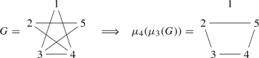
Example 3.5
If

then
so we have \(\underline{\textsf {CM}}^{\mathbb {Z}}(A_{\varepsilon }) \cong {\textsf {D}}^{\textsf {b}}({\textsf {mod}}\,k^4)\).
On the other hand, by applying the mutation \(\mu _1\), the relative mutations \(\mu _{2 \leftarrow 1}\) and \(\mu _{4 \leftarrow 1}\), \(G_\varepsilon \) becomes as follows:

Hence \(\alpha =1\) and \(\beta =3\) in the sense of Lemma 3.2, i.e., \(\mu _{4 \leftarrow 1}(\mu _{2 \leftarrow 1}(\mu _1(G_\varepsilon )))=G(1,3)\). This also shows \(\underline{\textsf {CM}}^{\mathbb {Z}}(A_{\varepsilon }) \cong {\textsf {D}}^{\textsf {b}}({\textsf {mod}}\,k^4)\).
4 Proof of Theorem 1.5
This section is devoted to the proof of Theorem 1.5.
For a graph G, let \({\text {Iso}}(G)\) be the set of isolated vertices of G and let \(i(G)=\#{\text {Iso}}(G)\).
For two graphs G and \(G'\), we write \(G \sim G'\) if G can be transformed into \(G'\) by finitely many mutations and relative mutations. By Lemmas 3.1 and 3.2, we know that \(G \sim G(\alpha ,\beta )\) for some \(\alpha \in \mathbb {Z}_{\ge 0}\) and \(\beta \in \mathbb {Z}_{>0}\). Moreover, by Lemma 3.3, we also see that \(G(\alpha ,\beta ) \not \sim G(\alpha ',\beta ')\) if \(\beta \ne \beta '\) and \(\beta ,\beta '>0\). (Note that this is not true if \(\beta =0\) or \(\beta '=0\). For example, \(G(2,0) \sim G(1,2)\).)
Here, we see the following:
Lemma 4.1
Assume that \(G \sim G(\alpha ,\beta )\) for \(\alpha \in \mathbb {Z}_{\ge 0}\) and \(\beta \in \mathbb {Z}_{>0}\). Then we have \(i(G') \le \beta \) for any graph \(G'\) with \(G \sim G'\).
Proof
If \(i(G')=0\), then the result is clear, so assume that \(i(G')\ge 1\). Notice that any relative mutation \(\mu _{v \leftarrow w}\) keeps the isolated vertices unchanged when v is not an isolated vertex. Thus, by Lemma 3.2, there is a sequence of relative mutations which transforms \(G'\) into \(G(\alpha ',\beta ')\) with \(\beta ' \ge i(G')\). Therefore,
Suppose that \(i(G')>\beta \). Then \(\beta ' \ge i(G') > \beta \), a contradiction. \(\square \)
We recall the following useful lemma on the point scheme \({\mathcal {E}}_{\varepsilon }\).
Lemma 4.2
(cf. [9, Theorem 2.3]) \({\mathcal {E}}_{\varepsilon }=\bigcap _{\varepsilon _{ij}\varepsilon _{jk}\varepsilon _{ki}=-1}{\mathcal {V}}(x_ix_jx_k)\subset \mathbb {P}^{n-1}\).
Let \(\ell _\varepsilon \) denote the number of irreducible components of \({\mathcal {E}}_\varepsilon \) that are isomorphic to \(\mathbb {P}^1\). For the investigation of \(\ell _\varepsilon \), we will recall some fundamental facts on the Stanley–Reisner ideals of simplicial complexes. Consult, e.g., [2, Section 5].
Let \(\Delta \) be a simplicial complex on the vertex set \(V=\{x_1,\ldots ,x_n\}\), i.e., \(\Delta \subset 2^V\) satisfies “\(F \in \Delta , F' \subset F \Longrightarrow F' \in \Delta \)”. A maximal \(F \in \Delta \) is said to be a facet of \(\Delta \). We define the Stanley–Reisner ideal \(I_\Delta \subset k[x_1,\ldots ,x_n]\) of \(\Delta \) as follows:
Clearly, \(I_\Delta \) is a squarefree monomial ideal. Conversely, every squarefree monomial ideal can be realized as a Stanley–Reisner ideal \(I_\Delta \) for some \(\Delta \).
For a facet F of \(\Delta \), let \(I_F\) be the prime ideal generated by all variables \(x_i\) with \(x_i \not \in F\), i.e., \(I_F=(x_i \mid x_i \in V {\setminus } F)\). It is known that
For the purpose of this section, for a graph G on the vertex set \(V:=V(G)=\{x_1,\ldots ,x_n\}\) with its edge set \(E:=E(G)\), we consider the squarefree monomial ideal \(I_G\) defined as follows:
In fact, we can easily see that \({\mathcal {V}}(I_{G_\varepsilon })={\mathcal {E}}_\varepsilon \).
Let \(\Delta _G\) be the associated simplicial complex, i.e., \(I_{\Delta _G}=I_G\). We write \(\ell (G)\) for the number of facets of \(\Delta _G\) with cardinality 2. By the primary decomposition (2), we see that
so we focus on the calculation of \(\ell (G)\). By definition of the Stanley–Reisner ideal, we have the following:
Assume that G contains an isolated vertex x. In this case, \(x_ix \not \in E\) and \(x_jx \not \in E\) hold for any \(\{x_i,x_j\} \subset V\) with \(x_ix_j \in E\). On the other hand, the condition
\(x_ix_j \not \in E\) such that “\(x_ix_k \in E\) and \(x_jx_k \in E\)” or “\(x_ix_k \not \in E\) and \(x_jx_k \not \in E\)”
for any \(x_k \in V {\setminus } \{x_i,x_j\}\)
is equivalent to \(N_G(x_i)=N_G(x_j)\). Hence, in the case G contains an isolated vertex, we see that
Notice that \(N_G(u)= \emptyset \) is equivalent to what u is an isolated vertex. Therefore, in the case G contains an isolated vertex, we conclude that
Let \(J(G)=\{\{x_i,x_j\} \subset V \mid N_G(x_i)=N_G(x_j) \ne \emptyset \}\) and let \(j(G)=\#J(G)\).
Example 4.3
If

then \(J(G_\varepsilon )=\{ \{1,3\}, \{2,4\} \}\) and \({\text {Iso}}(G_\varepsilon )=\{5,6\}\), so it follows that \(\ell _\varepsilon = \ell (G_\varepsilon )= 2+ \left( {\begin{array}{c}2\\ 2\end{array}}\right) =3\). In fact, we can verify that
and so \(\ell _\varepsilon =3\).
Lemma 4.4
Let G be a graph containing at least one isolated vertex. Assume that \(j(G)>0\). Let \(\{u_1,u_2\} \in J(G)\) and let \(u_2,\ldots ,u_m\) be all the vertices with \(N_G(u_1)=N_G(u_i)\) for \(i=2,\ldots ,m\). Let \(G'=\mu _{u_m \leftarrow u_1}(\cdots \mu _{u_3 \leftarrow u_1}(\mu _{u_2 \leftarrow u_1}(G))\cdots )\). Then \(j(G')< j(G)\) and \(\ell (G') \ge \ell (G)\).
Proof
Note that \(\{u_i, u_j\} \in J(G)\) for any \(1 \le i < j \le m\). It is easy to see that \(u_2,\ldots ,u_m\) become isolated vertices after applying \(\mu _{u_2 \leftarrow u_1},\ldots ,\mu _{u_m \leftarrow u_1}\). See below.

Thus \(i(G')=i(G)+m-1\). Moreover, we also see that \(J(G') = J(G) {\setminus } \{\{u_i,u_j\} \mid 1 \le i<j \le m\}\). In fact, since only the adjacencies of \(u_i\)’s and the adjacencies of the vertices in \(N_G(u_1)\) change after applying the above relative mutations, we only need to observe the vertices of \(N_G(u_1)\), but we can easily see that \(\{w,w'\} \in J(G)\) if and only if \(\{w,w'\} \in J(G')\) for any \(w,w' \in N_G(u_1)\).
Therefore, we conclude that \(j(G')< j(G)\) and
as required. (The inequality above follows from the inequality \(\displaystyle \left( {\begin{array}{c}a+b-1\\ 2\end{array}}\right) -\left( {\begin{array}{c}a\\ 2\end{array}}\right) -\left( {\begin{array}{c}b\\ 2\end{array}}\right) \ge 0\), which is true for any positive integers a, b.) \(\square \)
Example 4.5
Work with the same graph as in Example 4.3. Take \(\{1,3\} \in J(G_\varepsilon )\). Then 3 is the only vertex i with \(N_{G_\varepsilon }(1)=N_{G_\varepsilon }(i)\). Apply the relative mutation \(\mu _{3 \leftarrow 1}\) to \(G_\varepsilon \). Then \(G_\varepsilon \) becomes

Since \(J(G_{\varepsilon '})=\{ \{2,4\} \}\), we see \(j(G_{\varepsilon '})<j(G_\varepsilon )\). Moreover, apply \(\mu _{4 \leftarrow 2}\) to \(G_{\varepsilon '}\). Then \(G_{\varepsilon '}\) becomes G(1, 4). Hence \(\ell (G_\varepsilon ) \le \ell (G_{\varepsilon '}) \le \ell (G(1,4))=\left( {\begin{array}{c}4\\ 2\end{array}}\right) =6\).
Now let us prove Theorem 1.5.
Proof of Theorem 1.5
By [6, Lemma 6.5], mutation does not change the point scheme, so we may assume that \(G_\varepsilon \) is a graph containing an isolated vertex by Lemma 3.1. It follows from Lemma 3.2 that \(G_\varepsilon \sim G(\alpha ,\beta )\) for some \(\alpha \in \mathbb {Z}_{\ge 0}\) and \(\beta \in \mathbb {Z}_{>0}\). By the proof of Theorem 1.2, we see that \(r=\beta -1\). Thus our goal here is to prove that \(\ell _\varepsilon \le \left( {\begin{array}{c}\beta \\ 2\end{array}}\right) \). Applying Lemma 4.4 repeatedly, we can obtain a graph \(G'\) such that \(G' \sim G_\varepsilon \), \(j(G')=0\), and \(\ell (G') \ge \ell (G_\varepsilon )\). Since \(i(G') \le \beta \) by Lemma 4.1, we conclude by Lemma 4.4 that
as desired. \(\square \)
References
Artin, M., Tate, J., Van den Bergh, M.: Some algebras associated to automorphisms of elliptic curves. In: The Grothendieck Festschrift, vol. I, Progress in Mathematics, Birkhäuser, Boston, MA, vol. 86, pp. 33–85 (1990)
Bruns, W., Herzog, J.: Cohen–Macaulay Rings, Revised Edition. Cambridge Studies in Advanced Mathematics, vol. 39. Cambridge University Press, Cambridge (1998)
Buchweitz, R.-O.: Maximal Cohen–Macaulay modules and Tate cohomology over Gorenstein rings, unpublished manuscript (1985)
Godsil, C., Royle, G.: Algebraic Graph Theory. Graduate Texts in Mathematics, vol. 207. Springer-Verlag, New York (2001)
Knörrer, H.: Cohen–Macaulay modules on hypersurface singularities I. Invent. Math. 88, 153–164 (1987)
Mori, I., Ueyama, K.: Noncommutative Knörrer’s periodicity theorem and noncommutative quadric hypersurfaces, preprint, arXiv:1905.12266v2
Smith, S.P., Van den Bergh, M.: Noncommutative quadric surfaces. J. Noncommut. Geom. 7(3), 817–856 (2013)
Ueyama, K.: Noncommutative graded algebras of finite Cohen–Macaulay representation type. Proc. Am. Math. Soc. 143(9), 3703–3715 (2015)
Ueyama, K.: On Knörrer periodicity for quadric hypersurfaces in skew projective spaces. Can. Math. Bull. 62(4), 896–911 (2019)
Acknowledgements
The first author was supported by JSPS Grant-in-Aid for Early-Career Scientists 17K14177. The second author was supported by JSPS Grant-in-Aid for Early-Career Scientists 18K13381.
Author information
Authors and Affiliations
Corresponding author
Additional information
Publisher's Note
Springer Nature remains neutral with regard to jurisdictional claims in published maps and institutional affiliations.
Rights and permissions
Open Access This article is licensed under a Creative Commons Attribution 4.0 International License, which permits use, sharing, adaptation, distribution and reproduction in any medium or format, as long as you give appropriate credit to the original author(s) and the source, provide a link to the Creative Commons licence, and indicate if changes were made. The images or other third party material in this article are included in the article’s Creative Commons licence, unless indicated otherwise in a credit line to the material. If material is not included in the article’s Creative Commons licence and your intended use is not permitted by statutory regulation or exceeds the permitted use, you will need to obtain permission directly from the copyright holder. To view a copy of this licence, visit http://creativecommons.org/licenses/by/4.0/.
About this article

Cite this article
Higashitani, A., Ueyama, K. Combinatorial study of stable categories of graded Cohen–Macaulay modules over skew quadric hypersurfaces. Collect. Math. 73, 43–54 (2022). https://doi.org/10.1007/s13348-020-00306-1
Received:
Accepted:
Published:
Issue Date:
DOI: https://doi.org/10.1007/s13348-020-00306-1
Keywords
- Stable category
- Cohen–Macaulay module
- Noncommutative quadric hypersurface
- Adjacency matrix
- Stanley–Reisner ideal