
Abstract
Most decline curve methods have two main limitations; the model parameters as a rule are not functions of reservoir parameters and may yield unrealistic (nonphysical) values of expected ultimate recovery (EUR) because boundary-dominated flow may not develop in unconventional reservoirs. Over the past few years, several empirical models have emerged to address the second limitation, but they are challenged by the time to transition from infinite-acting flow period to the boundary-dominated flow. In this study, we performed statistical and model-based analysis of production data from hydraulically fractured horizontal oil wells and present a method to mitigate some of the limitations highlighted above. The production data were carefully analyzed to identify the flow regimes and understand the overall decline behavior. Following this step, we performed model-based analysis using the parallel flow model (sum of exponential terms), and the logistic growth model. After the model-based analysis, the model parameters were analyzed statistically and cross-plotted against available reservoir and well completion parameters. Based on the conclusion from the cross-plots and statistical analysis, we used design of experiments (DoE) and numerical reservoir simulations to develop functions that relate the model parameters and reservoir/well completion properties. Results from this work indicate that the production characteristics from these wells are highly variable. In addition, the parallel flow model indicates that there are at least two to three different time domains in the production behavior and that they are not the result of operational changes, such as well shut-in or operating pressure changes at the surface. All the models used in this study provide very good fits to the data, and all provide realistic estimates of EUR. The cross-plots of model parameters and some reservoir/well completion properties indicate that there is some relationship between them, which we developed using DoE and flow simulations. We have also shown how these models can be applied to obtain realistic estimates of EUR from early-time production data in unconventional oil reservoirs.
Introduction
According to Lee and Sidle (2010), decline curve analysis is the most widely used method of forecasting production from shale gas wells. The empirical decline curve equation presented by Arps (1945) has the following general form:
where q is the production rate, q i the initial production, D i the initial decline rate, and b is the derivative of the of D i and N p is the cumulative production.
In typical applications, Eq. 1 is fitted to the production data to determine parameters b and D i. Once the parameters are obtained, the equation is used to forecast the well/reservoir performance and also to estimate the ultimate recovery (EUR). When applied to unconventional production, the parameter b is often >1, which makes the cumulative production estimated from Eq. 2 at large time (t → ∞) to be infinite; that is, lim t→∞ N p(t) → ∞.
Fetkovich (1980) pointed out that any analysis with Eq. 1 that returned a b value >1 is a consequence of flow that is still dominated by transient effects. Several authors (Can and Kabir 2014; Ilk et al. 2008; Rushing et al. 2007) have pointed out that Eqs. 1 and 2 will yield optimistic results when applied to unconventional formations. Several authors (Harrell et al. 2004; Cheng et al. 2008) have suggested ways to overcome some of these problems. The different methods suggested by these authors have proved satisfactory but they lack a physical basis (Lee and Sidle 2010).
In recent years, more empirical models have been put forward to address the nonphysical reserves extrapolation problem of the Arps model when b > 1. Clark et al. (2011) introduced the logistic growth model, which has the desirable property of yielding physical values of reserves recovery. Ilk (2010), after analyzing production (rate) data from shale gas wells, developed a power-law model and a method of applying the model that arbitrarily switched from the power-law decline behavior to an exponential decline behavior. Duong (2011) also observed that a log–log plot of q/N p versus time was a straight line. Based on this observation, he developed a power-law type model and a procedure for its application. Valko (2010) presented an application of the stretched exponential decline model, a model which Johnston (2006) described as the expected decline function for a system that constrains many independently declining species, where each specie declines exponentially at a specific decline rate. All of these models were derived empirically; consequently, the model parameters are not functions of reservoir and/or well completion parameters.
This study has three main objectives: first, to understand the decline behavior and characteristics of oil wells by analyzing field production data (rate and wellhead pressures); second, to investigate the existence of a relationship between the empirical model parameters and the reservoir and/or well completion properties; third, to demonstrate the use of the relationship identified or developed in the second step in rate forecasting. This study explores the applications of both the logistic growth model and the parallel (sum of exponential terms) model.
Methodology
The data used for this study come from a liquid-rich shale play in North America. This dataset contains data from 80 wells of varying length and completion properties. These wells have also been on production for varying amount of time, ranging from 50 to 1500 days. Water production from these wells was relatively low, with average water cut ranging from 0.1 to 0.3. These high-frequency data are reported on a daily basis.
The work flow used for this study is summarized as follow:
-
1.
Analyze oil rate and well head pressure data to identify the predominant flow regime and signatures from this dataset.
-
2.
Perform model-based data analysis by fitting oil rate to empirical models to estimate the model parameters.
-
3.
Analyze and cross-plot the model parameters obtained in step 2 against available reservoir and well completion properties. This step enabled investigation of the existence of any relationship between the empirical model parameters and the reservoir and well completion properties.
-
4.
Use design of experiment (DoE) and numerical reservoir flow simulations to develop relationships between the model parameters and the reservoir and well completion properties.
Theoretical basis for flow regime identification
Wattenbarger et al. (1998) presented an application of the solution to the one-dimensional diffusivity (linear coordinates) equation for a closed rectangular boundary to facilitate analysis of production data in tight gas wells. The solution shows that for the constant pressure inner boundary condition, a log–log plot of rate versus time plots as a straight line with a slope of one-half at early times and as an exponential curve at late times. This solution is given by the following expression:
where q D is the dimensionless production rate and t D is the dimensionless time.
For the constant rate inner boundary condition, a log–log plot of wellbore pressure versus time also plots as a straight line with a slope of one-half and transitions to another straight line with unit slope. The solution for this case is given as
where p wD is the dimensionless pressure at the wellbore.
Plots of these solutions are presented in Fig. 1. The characteristics of these solutions have been observed in production data from many hydraulically fractured horizontal wells in unconventional formations. Patzek et al. (2014) analyzed production data from 8294 stimulated horizontal wells in North America and observed that the flow rate from these wells obeyed a simple scaling theory where the flow rate is proportional to the inverse of the square root of time.

A log–log plot of the solutions to the diffusivity equation in one dimension for a no-flow outer boundary condition. The dashed line represents the constant rate inner boundary condition, and the solid line represents the constant pressure inner boundary condition
Cinco-Ley and Samaniego (1981), Kuchuk and Biryukov (2014) and Bello (2009) have shown that a quarter slope on a log–log plot of rate versus time (constant pressure inner boundary condition) can be interpreted as the simultaneous linear flow of fluid in the fracture and reservoir matrix. We analyzed the dataset on this basis.
The dataset had production rates and tubinghead pressures. Consequently, we used the tubinghead pressure as a proxy for the bottomhole well flowing pressure by assuming that there is a constant pressure difference between the tubinghead pressure and the bottomhole pressure because of the pressure head of fluids in the wellbore. Figure 2 shows a typical dashboard from the flow regime identification exercise.

Diagnostic figures for a well in the dataset. a Log–log plot of oil rate versus time and the log–log plot of the tubinghead pressure versus time, b cross-plot of the oil rate versus tubinghead pressure
We make the following observations from the log–log plots of rate versus time and tubinghead pressure versus time for all the wells in the dataset:
-
1.
The rate–time plots showed slopes of one-half, one, one-and-a-half and exponential decline in no particular order. But in general the wells exhibit a power-law behavior with the one-half slope being the predominant slope observed.
-
2.
The plot of the tubinghead pressures versus time shows the existence of at least two-time scales in most of the wells. We make this conclusion because we observe a one-half slope followed by an exponential curve and this is followed by a constant tubinghead pressure. The exponential curve defines the fracture boundary, and the constant tubinghead pressure indicates flow from the reservoir matrix.
Model-based analysis
This section presents the results of model-based analysis. We considered two empirical models in this analysis, the logistic growth model and parallel flow model (sum of exponential terms). These models were fitted to rate and cumulative production data to obtain the model parameters, which were statistically analyzed. We then investigated the existence of any relationship between the model parameters and the reservoir and well completion properties by cross-plotting them against available well completion and reservoir properties.
The parallel flow model or sum of exponential model is based on the conception that when a horizontal well is hydraulically fractured, the reservoir rock is broken and subdivided into discrete blocks, each of which makes independent flow contribution to the fractures. The flow from each piece block is assumed to have an exponential decline, which is consistent with boundary-dominated flow. The mathematical expression for rate is then given by
where q T = production rate from the fractured horizontal well, \(q_{{{\text{i}}_{k} }}\) = initial production rate from the reservoir matrix element k, τ k = time constant for reservoir matrix k, defined mathematically as \(\frac{{v_{\text{p}} c_{\text{t}} }}{J}\), v p is the matrix pore volume, c t is the total matrix compressibility and J is the productivity index of the matrix. This definition is identical to that used in the capacitance–resistance model, espoused by Sayarpour et al. (2009), Nguyen (2012), Cao et al. (2014).
Logistic growth models are often used to model growth (population, market penetration of new products and technologies) Tsoularis and Wallace (2002). Clark et al. (2011) presented the first application of the logistic growth model in production forecasting in unconventional reservoirs. The logistic growth model is given as
where N = carrying capacity, a = constant, n = hyperbolic exponent and t = time.
An expression for production rate, q, is obtained by differentiating Eq. 6 with respect to time:
Clark et al. (2011) described the carrying capacity in Eqs. 6 and 7 as the estimated ultimate recovery for a well without an economic constraint, and it acts as an upper limit on the cumulative production. Note that N p → N because t → ∞.
For the parallel flow model, the model parameter estimation was done by minimizing the problem defined below
where \(f_{k} = \frac{{q_{{{\text{i}}_{k} }} }}{{q_{{{\text{i}}_{T} }} }}\); \(q_{{{\text{i}}_{T} }}\) is the maximum value of production rate in the dataset.
In formulating the model fitting problem in Eq. 8, we have normalized the model and data with the maximum value of production rate and then included the constraint such that the coefficient of the exponential terms must be fractions that sum up to 1. The objective of this formulation is that we do not have to specify the number of exponential terms in the model beforehand, that is, N e can be set to large number and the optimization process would return a value for N e that will give the best fit to the data. The number of terms required is obtained by determining the number of fractional coefficient (f k ) of the exponential terms that are not equal to zero. The model was fitted to data by finding values of f k and τ k that minimize Eq. 8.
For the logistic growth model, we applied Eqs. 6 and 7 to the dataset by finding the values of the model parameters that minimized the squared difference between model predictions and field data.
Results of model-based analyses
Example application of parallel flow model
In estimating the model parameters with the parallel flow model, N e (the number of exponential terms) was initially set equal to four. An example application of the model to a well (UT-ID4) in the dataset is in Fig. 3. As shown in Fig. 3a, the parallel flow model gives a good fit to production data. Figure 3b shows that the coefficient of determination is large at a value of 0.94. Figure 3d is a plot of the error versus time; error is defined as the difference between the model predictions and data. The error is larger at early time because there is more scatter in the data at early time compared to late time. A summary of the model parameters obtained for this case is in Table 1.

Example application of the parallel flow model. a Normalized rate/time plot for the data and model history match and c normalized rate/cumulative plot for the data and model history match. b Cross-plot of the normalized rate data and the normalized model rate prediction. d Plot of the error in normalized rate prediction (q D-Data − q D-Model) versus time
This well only needs two exponential terms in the parallel flow model to obtain a good fit with data. In all likelihood, the initial condition contributed to the fact that f 2 and f 3 turned out to be zero. The estimated EUR for this well is 1.77 × 10⁵ STB.
Results of statistical analysis of model parameters: parallel flow model
After applying the parallel flow model to all the 87 wells in the dataset, we observed that 58 wells required only three exponential terms, 28 wells required only two exponential terms, and only one well required four exponential terms. Figure 4 presents the resulting distribution of the fitting parameters. Specifically, Fig. 4a, c, e presents the distribution of initial production rates for each term in the parallel flow model that was not equal to zero. From these figures, we conclude that all of the distributions are log-normal; therefore, initial production rates with values close to the mean value are more frequent than initial production rates with high values. Figure 4b, d, f is the corresponding distributions of time constants for the initial productions rates in Fig. 4a, c, e, respectively. The distributions of the time constants also appear to follow a log-normal distribution. The values of the time constants in Fig. 4d, f appear to have the same order of magnitude with mean values of 4.7 × 10⁴ and 4.1 × 10⁴, respectively. The values of time constants in Fig. 4d, f appear to be an order of magnitude greater than those in Fig. 4b, and the mean value of the time constants in Fig. 4b is 381. This observation suggests that the time constants in Fig. 4d, f are from the same distribution and the time constants in Fig. 4b are from another distribution.

Probability density function (PDF) and cumulative distribution function (CDF) obtained for the parallel flow model applied to the dataset
Physically, the time constants can be interpreted as a measure of how fast the fluids in a reservoir would drain; small values indicate that the fluids would drain very fast and large values imply that it would take a longer time for the fluids to drain from the reservoir (Ogunyomi et al. 2016). Based on this definition of the time constant, we can state that there are at least two-time scales in the dataset, one-time scale accounts for the high-transmissivity, low-storativity fractures (τ 1) and the second-time scale accounts for the low-transmissivity, high-storativity reservoir matrix (τ 2 and τ 3).
Table 2 presents the statistical summary of the model parameters for the parallel flow model. The range of each of parameter in this table is quite large, thereby indicating that there is a great degree of variability in well performance in this dataset.
Example application of logistic growth model
Figure 5 presents an example application of the logistic growth model to the same well in the dataset. This figure suggests that the coefficient of determination is high with a value of 0.83, but not as large as 0.94 obtained with the parallel flow model. Data scatter at early times increases the error bounds. Table 3 summarizes the model parameters.

Example application of the logistic growth model. a Rate–time plot for the data and model history match and c rate–cumulative plot for the data and model history match. b Cross-plot of the normalized rate data and the normalized model rate prediction. d Plot of the error in rate prediction (q Data − q Model) versus time
The carrying capacity obtained for this well is 1.1 × 10⁵ STB; therefore, the EUR from this well based on the logistic growth model is 1.1 × 10⁵ STB.
Results of statistical analysis of model parameters: logistic growth model
Figure 6 presents the distribution (PDF and CDF) of the model parameters obtained for the logistic growth model. A general observation from this figure is that they all appear to be log normally distributed.

Probability density function (PDF) and cumulative distribution function (CDF) obtained for the logistic growth model applied to the dataset. a PDF and CDF for the carrying capacity, b PDF and CDF for the hyperbolic exponent and c PDF and CDF for the constant a
Table 4 presents the statistical summary of the logistic growth model parameters for wells in the dataset. The mean value of the carrying capacity is 1.3 × 10⁵ with a standard deviation of 6.9 × 10⁴. It has a range of 4.1 × 10⁵. The hyperbolic constant and the constant a have mean values of 0.62 and 5897, respectively. The range of n and a is 2.13 and 4.8 × 10⁵, respectively. This outcome can also be interpreted as the result of high degree of variability in well performance.
Correlation between model parameters and the reservoir and well completion properties
We investigate the existence of any relationship between the model-derived parameters and the reservoir and well completion properties with two methods. For the first method, we investigated the existence of a linear relationship by computing the correlation coefficient between the variables. Navidi (2008) defined the correlation coefficient ρ as a measure of the degree of linear relationship between two variables, and it varies between +1 and −1. A value of +1 implies a strong positive linear relationship, whereas a value of −1 means a strong negative linear relationship. A value of zero suggests that there is no linear relationship between the two variables.
With the second method, nonlinear relationships were investigated by making cross-plots of the model parameters (including its transforms) and the reservoir and well completion properties. These cross-plots are then evaluated for any recognizable functional relationship.
Parallel flow model
The computed correlation coefficients for the parallel flow model and the reservoir and well completion properties are summarized in Table 5 in which we have highlighted values of |ρ| ≥ 0.2.
This table suggests that the initial production rates show some level of correlation with most of the reservoir and well completion properties. In contrast, the time constants does not show the same level of correlation.
Logistic growth model
Table 6 presents the computed correlation coefficients between the model parameters and the reservoir and well completion properties. In this table, we have highlighted |ρ| ≥ 0.2. Based on these criteria, the carrying capacity possibly has a linear relationship with well spacing, porosity, average injection pressure, total injected fluid and the mass of sand injected. The fact that the carrying capacity correlates with well spacing and porosity suggests that there is a relationship between the carrying capacity and the drainage volume of the well. The hyperbolic constant n and the constant a do not have any linear relationship with the reservoir and well completion properties. No obvious nonlinear relationship emerged from the cross-plots.
Development of mathematical relationships between empirical model parameters and reservoir and well completion properties
The results of the statistical analysis of the model parameters in the previous sections show that the model parameters correlate to some degree with the reservoir and well completion properties. In this section, we use design of experiment (DoE), numerical reservoir simulation and response surface modeling (RSM) to develop functional relationships between the model parameters and the reservoir and well completion properties. More details on the theory of DoE and RSM can be found in Box et al. (2005) and Myers and Montgomery (2002).
We developed the functional relationship by:
-
1.
Generating data from numerical reservoir simulation where we built the numerical simulation models based on the result of a fractional factorial design experiment. We used a \(2_{VI}^{9 - 2}\) fractional–factorial design, which resulted in 256 numerical reservoir simulation runs. The reservoir and well properties used for this experiment are in Table 7. Figure 7 is a schematic representation of the process described , and Fig. 8 is one of the numerical simulation models used for data generation.
Table 7 Reservoir and well completion properties used in the fractional factorial design of experiments used to build the numerical simulation model Fig. 7 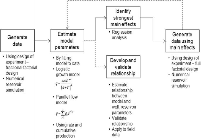
Schematic diagram of the process used in developing the mathematical relationship between the model parameter and the reservoir and well completion properties
Fig. 8 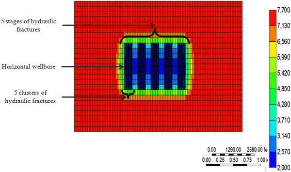
Pressure distribution in one of the numerical simulation models and showing the number of fracture stages and the number of hydraulic fracture clusters
-
2.
After generating the synthetic data, we estimated the parameters for the empirical models (logistic growth and parallel flow model) by fitting them to data using the method described earlier. Rate and cumulative production data were used in the fitting exercise.
-
3.
Identify the reservoir and well completion properties that have the strongest effects on each parameter in the empirical models. We identified the strongest effects by performing regression analysis on each parameter in the empirical model and all the variables in Table 7. Using the t statistic from the regression analysis, we eliminate those variables whose coefficient is most likely equal to zero based on their P values. The P value is the probability that the coefficient of a variable is equal to zero. The larger the P values the more likely the coefficient is equal to zero and the smaller it is the less likely the coefficient is equal to zero. A P value of 0.0001 was chosen as cutoff, if the P value is >0.0001, the coefficient of that variable is not significantly different from zero and we can eliminate such variables from further analysis.
Table 8 provides a summary of the result of this step; the solid dots indicate that the reservoir/well property that has a strong effect on the value of the corresponding model parameter. For example, fracture half-length has a strong effect on the value of the carrying capacity for the logistic growth model.
Table 8 Summary of reservoir and well properties that have the strongest effect on the model parameters -
4.
After step 3, we have a list of variables that have the strongest effect on each model parameter. We then performed a full factorial design of experiment with the variables in this list for each model parameter and then build the numerical reservoir model to generate data with those results. Note that the unimportant properties were kept unperturbed at their expected values. Table 9 presents the design table for the carrying capacity N; this design is for a 23 full factorial experiment with 8 numerical simulation models.
Table 9 Design table for variables with the main effect on the carrying capacity, N


Because the constant a has all its main effect variables in common with the hyperbolic constant, we used the same design table for their experiments. Table 10 is the design table for n and a, and the experiment design was for a 24 full factorial design with 16 numerical simulation models. We also combined the design table for the parallel flow model parameters because they have many of the main effects variables in common. The design for the parallel flow model parameters was a 27 full factorial design with 128 numerical simulation models.
-
5.
Repeat step 2 to obtain the model parameters that would be used to develop the response surface function.
-
6.
Using regression analysis. we develop a functional relationship between each of the model parameters and the reservoir and well completion properties. The developed relationship is then validated with synthetic examples.
The results obtained for step 6 are presented below.
Logistic growth model
Carrying capacity, N
Equation 9 is the response surface function for carrying capacity that shows a relationship between the carrying capacity and the reservoir thickness (h), well length (L w) and the fracture half-length (x f). Different transformations of the carrying capacity were evaluated; we chose the transformation that gave the largest coefficient of variation when the model predictions are cross-plotted against actual values. This transformation has a coefficient of variation of 0.95. Figure 9a shows a cross-plot of the predicted values of carrying capacity using Eq. 9 and the actual values. Figure 9b presents the residuals plotted on a normal probability graph, wherein the straight-line signature indicates normal distribution. Figure 10a, b is response surfaces constructed with Eq. 9, and they show how the carrying capacity varies with the changes in independent variables. Note that Fig. 10a reflects the response surface when the fracture half-length is at its smallest value, whereas Fig. 10b shows the same when the fracture half-length is at its largest value.

Validation of developed relationship for carrying capacity. a Cross-plot of the predicted values carrying capacity versus the actual values of the carrying capacity. b Diagnostic plot that shows that the residuals of the regression are normally distributed

Response surfaces for carrying capacity
Hyperbolic exponent, n
Equation 10 is the developed relationship between the hyperbolic exponent and the reservoir and well properties. A linear relationship has the highest coefficient of variation of 0.95 when compared to the other transformations evaluated. We evaluated a linear, quadratic, power and logarithmic transforms.
Constant, a
Equation 11 is the relationship developed for the constant a. This relationship had the highest coefficient of variation of 0.81 from the transforms evaluated.
Parallel flow model
Initial production rate one, q i1
Equation 12 is the response surface function for the initial production rate, q i1. It shows a relationship between the initial production rate one and the reservoir thickness (h), fracture permeability, matrix permeability, porosity, well length (L w), initial reservoir pressure and the bottomhole flowing pressure. Different transformations of the initial production rate one were evaluated, and the transformation that gave the highest value of coefficient of variation is the natural-log transform. This transformation has a coefficient of variation of 0.98.
Time constant one, τ 1
Equation 13 is the response surface function for time constant one, τ 1. A power transformation gave the highest value of coefficient of variation when the model predictions are cross-plotted against actual values. This transformation has a coefficient of variation of 0.73.
Initial production rate two, q i2
Equation 14 is the response surface function for initial production rate two, q i2. It shows a relationship between the initial production rate two and the reservoir thickness (h), fracture permeability, matrix permeability, porosity, well length (WL), initial reservoir pressure and the bottomhole flowing pressure. The log transformation gave the highest coefficient of variation of 0.99.
Time constant two, τ 2
Equation 15 is the response surface function for time constant two, τ 2. A power transformation gave the highest value of the coefficient of variation when the model predictions are cross-plotted against actual values. This transformation has a coefficient of variation of 0.82.
Discussion
Both models used in this study can predict the EUR; for the logistic growth model the carrying capacity is a parameter in the fitting, and for the parallel flow model the function converges to a finite value when extrapolated to infinity. Because both methods require numerical fitting of model parameters, neither offers a clear advantage over the other. The logistic growth model does not have physically meaningful parameters (except for the carrying capacity) and does not fit the data as well as does the parallel flow model, although both results in good fits. Note that the parallel flow model has more parameters, four for the two-compartment model, as opposed to three for the logistic model. Therefore, the latter approach is less likely to result in nonunique solutions. The logistic model does not have the multiple scales that are such a prevalent feature of the data.
The model-based analysis with the parallel flow model clearly indicates the existence of multiple-time scales in the production profiles of these wells. The parallel flow model is based on the concept that the reservoir contains multiple independently declining reservoir elements (compartments) that have different and unique time constants, representing declining characteristics. Therefore, when two or more reservoir compartments are present, this will be reflected in the number of terms in the parallel flow model. The observed time scales also highlight the importance of high-frequency data and integrating all available information in analyzing production data. Most analysis techniques ignore the early-time production data (which we included in our analysis) because of wellbore effects (wellbore storage or skin and flow back of fracture fluids) and noise, thereby missing the first-time scale and only analyzing data that are dominated by production from the second-time scale. While it is possible that these phenomena affect early-time production only, it does not eliminate the possibility of analyzing early-time data to estimate the dimensions of the reservoir element/compartment (this could be the fracture or fracture network) that accounts for early-time flow. Ogunyomi (2014) presented a rate–time relation capable of modeling flow from a double-porosity model that typically exhibits two-time scales. The model they presented is also valid for early- and late-time flow (transient and boundary-dominated flow).
Analysis of the model parameters for the logistic growth and parallel flow models showed that they have some correlation with the reservoir and well completion properties. For example, the carrying capacity in the logistic growth model correlated with the well spacing, total fluid injected and the mass of sand injected. In an ideal situation, these properties can be used to define the drainage volume of a well. It therefore seems reasonable, as suggested by Clark et al. (2011), to use the carrying capacity as a constraint on the recoverable reserves from a well.
Conclusions
This study presents the results of a detailed statistical and model-based analysis of production data from an unconventional oil reservoir. We also analyzed this production dataset to identify different flow regimes and flow signatures using the linear flow concept. The following conclusions appear pertinent based on the results of these analyses:
-
1.
Production performance from wells in unconventional reservoirs should be expected to be highly variable. The production signatures show varying slopes on a diagnostic log–log plot that ranges from one-half to one-and-a-half. However, the one-half slope signature dominated in most cases. This observation corroborates the notion that 1D linear flow is adequate in modeling recovery from these reservoirs although this might underestimate production because it ignores the first-time scale.
-
2.
The analysis showed that at least two exponential terms of the parallel flow model are needed to adequately model production from these reservoirs. A statistical analysis of the time constants confirms that there are two distributions of time constants. Therefore, we can conclude that there are at least two-time scales in the production history from these wells. An important corollary of this observation is that any forecasting effort that does not account for the multiple-time scales will result in conservative EUR predictions.
-
3.
Based on the general observation that the parameters from the empirical models correlated with the reservoir and well completion properties in the dataset, we developed functions that relate the model parameters to reservoir and well properties by using design of experiments and numerical reservoir flow simulations. If the reservoir and well properties are known, these relations can be used to compute the model parameters, which can then be used in the models to forecast production profiles. Of course, these relations are only valid within the range that was used to develop them.
Abbreviations
- τ 1 :
-
Time constant one (days)
- τ 2 :
-
Time constant two (days)
- D i :
-
Initial decline rate (day−1)
- b :
-
Derivative of inverse of initial decline rate (unitless)
- q i :
-
Initial production rate (STB/D)
- N p :
-
Cumulative production (STB)
- q D :
-
Dimensionless flow rate (dimensionless)
- t D :
-
Dimensionless time (dimensionless)
- p wD :
-
Dimensionless wellbore pressure (dimensionless)
- q T :
-
Production rate from fractured horizontal well (STB/D)
- N e :
-
Number of discrete reservoir elements (unitless)
- \(q_{{{\text{i}}_{k} }}\) :
-
Initial production rate from reservoir element k (unitless)
- τ k :
-
Time constant for reservoir element k (days)
- N :
-
Carrying capacity (STB)
- a :
-
Constant a
- n :
-
Hyperbolic constant (unitless)
- M :
-
Number of data points (unitless)
- t :
-
Time (days)
- f m :
-
Normalized data initial production rate (fraction)
- f k :
-
Normalized model initial production rate (fraction)
- k f :
-
Fracture permeability (md)
- k m :
-
Matrix permeability (md)
- L w :
-
Well length (ft)
- p i :
-
Initial reservoir pressure (psi)
- p wf :
-
Wellbore flowing pressure (psi)
- h :
-
Reservoir thickness (ft)
- φ :
-
Porosity (fraction)
References
Arps JJ (1945) Analysis of decline curves. SPE-945228-G. Trans AIME 160:228–247
Bello RO (2009) Rate transient analysis in shale gas reservoirs with transient linear behavior. Ph.D. Dissertation, Texas A&M University, College Station
Box GE, Hunter JS, Hunter WG (2005) Statistics for experimenters. Wiley, London. ISBN 0-471-71813-0
Can B, Kabir CS (2014) Containing data noise in unconventional reservoir performance forecasting. JNGSE 18(2014):13–22. doi:10.1016/j.jngse.2014.01.010
Cao F, Luo H, Lake LW (2014) Development of a fully coupled two-phase flow based capacitance–resistance model (CRM). Paper SPE-169485-MS presented at the SPE improved oil recovery symposium, Tulsa, 12–16 April. doi:10.2118/169485-MS
Cheng Y, Lee WJ, McVay DA (2008) Improving reserves estimates from decline-curve analysis of tight and multilayer gas wells. SPEREE 05:912–920. doi:10.2118/108176-PA
Cinco-Ley H, Samaniego VF (1981) Transient pressure analysis: finite conductivity fracture case, damaged fracture case. Paper SPE-10179-MS presented at the SPE annual technical conference and exhibition, San Antonio, 4–7 October. doi:10.2118/10179-MS
Clark AJ, Lake LW, Patzek TW (2011) Production forecasting with logistic growth models. Paper SPE 144790 presented at the SPE annual technical conference and exhibition, Denver, 30 October–2 November. doi:10.2118/144790-MS
Duong AN (2011) Rate-decline analysis for fracture dominated shale reservoirs. SPEREE 14(03):277–387. doi:10.2118/137748-PA
Fetkovich MJ (1980) Decline curve analysis using type curves. JPT 32(6):1065–1077. doi:10.2118/4629-PA
Harrell DR, Hodgin JE, Wagenhofer T (2004) Oil and gas reserves estimates: recurring mistakes and errors. Paper SPE-91069-MS presented at the SPE annual technical conference and exhibition, Houston, 26–29 September. doi:10.2118/91069-MS
Ilk D (2010) Well performance analysis for low to ultralow permeability reservoir systems. Ph.D. Dissertation, Texas A&M University, College Station
Ilk D, Rushing JA, Perego AD, Blasingame TA (2008) Exponential vs. hyperbolic decline in tight gas sands—understanding the origin and implications for reserve estimates using Arps decline curves. Paper SPE-116731-MS presented at the SPE annual technical conference and exhibition, Denver, 21–24 September. doi:10.2118/116731-MS
Johnston DC (2006) Stretched exponential relaxation arising from a continuous sum of exponential decays. Phys Rev B 74:184430. doi:10.1103/PhysRevB.74.184430
Kuchuk F, Biryukov D (2014) Pressure transient behavior of continuously and discretely fractured reservoirs. SPEREE 17(1):82–87. doi:10.2118/158096-PA
Lee WJ, Sidle RE (2010) Gas reserves estimation in resource plays. SPE Econ Manag 2:86–91
Myers RH, Montgomery DC (2002) Response surface methodology: process and product optimization using design of experiments. Wiley, London. ISBN 0-470-17446-3
Navidi W (2008) Statistics for engineers and scientists. McGraw-Hill, New York. ISBN 978-0-07-337633-2
Nguyen AP (2012) Capacitance resistance modeling for primary recovery, waterflood, and water/CO2 flood. Ph.D. Dissertation, The University of Texas at Austin, Austin
Ogunyomi BA (2014) Mechanistic modeling of recovery from unconventional reservoirs. Ph.D. Dissertation, The University of Texas at Austin, Austin
Ogunyomi BA, Patzek T, Lake LW, Kabir CS (2016) History matching and rate forecasting in unconventional oil producing reservoirs using an approximate analytical solution to the double-porosity model. SPEREE 19(1):70–82. doi:10.2118/171031-PA
Patzek TW, Male F, Marder M (2014) Gas production from Barnett shale obeys a simple scaling theory. Proc Natl Acad Sci USA 110(49):19731–19736. doi:10.1073/pnas.1313380110
Rushing JA, Perego AD, Sullivan RB, Blasingame TA (2007) Estimating reserves in tight gas sands at hp/ht reservoir conditions: use and misuse of an Arps decline curve methodology. Paper SPE 109625 presented at the SPE annual technical conference and exhibition, Anaheim, 11–14 November. doi:10.2118/109625-MS
Sayarpour M, Zuluaga E, Kabir CS, Lake LW (2009) The use of capacitance–resistance models for rapid estimation of waterflood performance and optimization. JPSE 69(2009):227–238
Tsoularis A, Wallace J (2002) Analysis of logistic growth models. Math Biosci 179(1):21–55
Valko PP (2010) A better way to forecast production from unconventional gas wells. Paper SPE 134231-MS presented at the SPE annual technical conference and exhibition, Florence, 19–22 September. doi:10.2118/134231-MS
Wattenbarger RA, El-Banbi AH, Villegas ME, Maggard JB (1998) Production analysis of linear flow into fractured tight gas wells. Paper SPE-39931-MS presented at the SPE rocky mountain regional/low-permeability reservoirs symposium and exhibition, Denver, 5–8 April. doi:10.2118/39931-MS
Acknowledgements
The sponsors of the Center for Petroleum Asset Risk Management (CPARM) at the University of Texas at Austin supported this work. We thank Hess Corporation for providing data for this work and the Computer Modeling Group (CMG) for use of their black oil simulator. Larry W. Lake holds the Sharon and Shahid Ullah Chair at the University of Texas at Austin.
Author information
Authors and Affiliations
Corresponding author
Rights and permissions
Open Access This article is distributed under the terms of the Creative Commons Attribution 4.0 International License (http://creativecommons.org/licenses/by/4.0/), which permits unrestricted use, distribution, and reproduction in any medium, provided you give appropriate credit to the original author(s) and the source, provide a link to the Creative Commons license, and indicate if changes were made.
About this article

Cite this article
Ogunyomi, B.A., Dong, S., La, N. et al. An approach to modeling production decline in unconventional reservoirs. J Petrol Explor Prod Technol 8, 871–886 (2018). https://doi.org/10.1007/s13202-017-0380-9
Received:
Accepted:
Published:
Issue Date:
DOI: https://doi.org/10.1007/s13202-017-0380-9