Disaggregation of the electric loads of small customers through the application of the Hilbert transform

Abstract

This paper is intended to explain how the possibilities of enabling technologies (advanced metering infrastructures) can be expanded on to evaluate end uses at the demand-side level. For example, these data allow validating the effective response to market prices (energy markets) or system events (demand response), and besides, the possibilities that energy efficiency offers (in capacity markets), mainly under the supervision of a load aggregator. Hilbert transform properties along with other mathematical tools are used to extract the characteristics of the more suitable uses for demand response policies from the aggregated load demand of the user. This is achieved without complex statistical analysis of the demand loads. The tool filters pulse waveforms (in this case, the components of daily demand) and provides the aggregator the main characteristics of load, both in normal state or under response to system events or market prices.

Introduction

A basic European Commission “20–20–20” support policy on Energy (European Commission 2011) would like 80 % of consumers to have smart meter devices by 2020. This objective will require the deployment of 130–150 million new smart meters by 2020, which equals a total market of $24–26 billion (Greenbang 2012).

The problem is that the high potential of smart metering may not be beneficial for consumers if they are not well informed about the benefits and possibilities of these technologies. Furthermore, if the markets are closed to the demand side or if they create barriers for some customer segments, some users will not get involved in energy policies (Faruqui et al. 2010). Moreover, customers need to be motivated and “cultured” to develop the potential benefits that are possible thanks to the deployment of these “enabling” technologies in this new decade. While policymakers have focussed on rolling out smart meters, little attention has been paid to the issue of what are the benefits and possibilities of smart meters for the customer. Only with the involvement and active participation of the customers [demand response (DR) and energy efficiency (EE)] can the 2020 objectives be attained. The last analysis of European Council about 2020 objectives points out the fact that “the Union is not on track to achieve its energy efficiency targets” (European Parliament and Council 2012).

Moreover, EU customers have to overcome education and technical barriers to actually obtain the maximum potential out of DR and, in this way, directly access the energy markets. These residential segments in 2010 stand for 29.71 % of the overall electricity demand in EU-27 (Bertoldi et al. 2012). Therefore, more knowledge and experience has to be acquired, and the new information made available with the deployment of smart meters and “enabling” technology in the EU and USA (Piette et al. 2007; Johnson Controls 2010) must be used. The problem with this information (at least, in terms of the measurement of real and reactive power with pacer from 1 to 5 min) is that the specific demand share of end uses and their behaviour are difficult to evaluate. This is not an easy task, especially for cycling loads such as space heating, air conditioning and water heating, which are the first candidates to be used for DR given their inherent capacity to store electrical energy in heat, cold or hot water.

This paper proposes a new method for achieving the disaggregation of the overall load of a residential customer (i.e. with the information available with the future deployment of smart meters), to ascertain the main characteristics of these loads, and further use these data for DR and EE purposes. The tool carries out its objectives through the use of Hilbert transform HT properties combined with statistical analysis. HT properties allow determining changes in the operation cycling frequency of the loads before, during and after a DR control policy is applied. Statistical analysis of the instantaneous amplitude of the signal obtained through HT provides the power level and width pulse of the signal, getting this way an accurate estimation of the load from the aggregated original load data.

This way, by measuring aggregated load when DR is applied (for instance, in response to prices or system events), the aggregator can evaluate (short term) and demonstrate the system operator SO (medium term) that their customers are responding with the change in load consumption without having to establish an intricate baseline with complex physical or statistical tools, or deploy additional measurement resources. The tool this way is simpler requiring only the knowledge of the load under control for feedback purposes. This underdeveloped potential could be very useful to promote the demand aggregator figure (Johnson Controls 2010).

This paper is structured as follows: “Load disaggregation” briefly presents the need for the load signature analysis; “Hilbert transform” deals with the Hilbert transform as being the preferred tool to analyse non-stationary signals, and it discusses the more common drawbacks and advantages; “Demodulation of square waveforms” introduces the demodulation process and discusses the information that can be extracted through the instantaneous frequency and amplitude analysis of square/pulse waves; “Demand response evaluation” shows how concepts explained in “Demodulation of square waveforms” are applied to real demand profiles for a representative residential customer. Finally, “Conclusions” presents the conclusions.

Load disaggregation

Energy evaluation for efficiency and demand response programmes requires determining the percentage and characteristics of each end use. The importance of these end uses, their inherent response capacity and the time in which the use changes from ON to OFF states or vice versa (power ON or OFF) are required to build a model for the customer, or to validate physically based load models (Koponen 2012). This can also be used to determine which policies are the most effective: load retrofit, technology change, curtailment capacity, the change of time of use or the evaluation of the demand elasticity (Faruqui et al. 2013). Usually, the utilities and aggregators have power measurements at a central point. In this way, the easiest way to evaluate final end uses is to insert an intermediate monitoring device between the plug and the appliance; then, its use and dynamics are recorded. This method is known as “intrusive monitoring”. It is still an expensive method and should be studied in detail (cost vs. effectiveness) for large scale deployment (Gomatom and Homes 2012).

The evolution of technology and the public authorities’ support of advanced metering infrastructure (AMI) add value to the use of this new capacity of measurement. For instance, the use of smart meters allows to make estimations at the customer metering point without having to access to individual sockets. This is usually called “non-intrusive load monitoring” (Zeifman and Roth 2011) (NILM, NIALM). In the last decades, new assessment tools have been proposed and tuned to obtain the so-called “load signatures” (LS) (Liang et al. 2010a, b) from power and waveform measurements at the customer level, for example during transient events (Chang 2012). With these LS, the load composition for an end user can be estimated.

Usually, LS are classified in micro- and macro-level signatures (Liang et al. 2010a, b). Every measurement with a pacer faster than one sample per cycle (20 ms at 50 Hz) is considered to be at micro-level, where the characteristics of voltage and current waveforms are identified (for instance, load harmonics). A measurement with a pacer slower than one sample per cycle is considered to be at macro-level (i.e. we are finding load changes or load steps in active and reactive power). This last level was the first possibility studied for load disaggregation (Hart 1992).

One objective of this paper is to find “macro-level” LS for the end uses with the higher potential for DR and EE. In small customer segments and according to the literature reports in the USA (Piette et al. 2007) and the EU, these end uses are commercial and residential heating and cooling loads, water heating, lighting and refrigerators. Figure 1a and b shows actual “natural/own” demand, and Fig. 1c shows “forced” power consumption for space heating.

Fig. 1

Demand monitoring. a Natural duty cycles for water heater. b Continuous demand for inverter heat pump load. c Natural and forced duty cycles for space-heating load. d Daily demand for a residential customer

Figure 1d shows the same waveform embedded at the customer metering point recorded by a low-price electronic meter (main characteristics: price < €250; maximum pacer trigger, one sample per minute; four input channels: voltage, current and P&Q powers, with a data storage capacity of about 1 GB). It is not trivial to identify the heating-space load working at the same time as other loads demand energy (in our case: fridge, electric heater, washing machine, electronic appliances, heat pump, water heater or lighting).

Literature shows examples of NILM at both the macro- and micro-levels (Hart 1992; Liang et al. 2010a, b). These works propose the use of Fourier series, neural networks, spectral envelopes, power changes and other waveform features. There are other works based on hidden Markov models (HMMs) (Elliott et al. 1995) for load disaggregation (Kim et al. 2011; Kolter 2011). However, HMM does not work well if an individual load changes its load pattern due to DR policies. In addition, HMM need a statistical study of the individual loads of the residential user under analysis. Our approach is more specific as we do not try to disaggregate each load present in the aggregated load curve, but to detect key factors (power, frequency and t _ON times) of the loads more suitable for DR and evaluate the effectiveness of DR and EE policies in the customer side.

Our research is based on the Hilbert transform (HT), a mathematical tool that has been used in power systems to solve other problems (Browne et al. 2008; Senroy et al. 2007). HT has not been used previously for the analysis of pulse/square load waveforms. This paper will demonstrate how HT can be used and tuned for this purpose. The advantage of our approach is that it can extract and filter pulse/square waveforms from an aggregate load while providing all the necessary information to reconstruct the individual appliance demand: cycling frequency, ON/OFF times, amplitude and dynamics of these magnitudes.

Hilbert transform

For any real time series g(t), the HT is defined as Eq. 1:

$$ H\left(g(t)\right)=\frac{1}{\pi}\mathrm{PV}{\displaystyle \underset{-\infty }{\overset{\infty }{\int }}\frac{g(u)}{t-u}\mathrm{d}u} $$

(1)

where PV stands for the Cauchy principal value of the singular integral. After the Hilbert transform is defined, its analytic signal (the time series and its transform) can be defined as Eq. 2:

$$ s(t)=g(t)+ jH\left(g(t)\right) $$

(2)

where H[g(t)] is the Hilbert transform of g(t).

The analytic signal can be presented in its exponential form as Eq. 3:

$$ s(t)=A(t){e}^{j\theta (t)} $$

(3)

where A(t) is the instantaneous amplitude and θ(t) the instantaneous phase.

The instantaneous frequency f(t) or instantaneous pulse w(t) can be defined as Eq. 4:

$$ f(t)=\frac{w(t)}{2\pi }=\frac{1}{2\pi}\frac{\mathrm{d}\theta (t)}{\mathrm{d}t} $$

(4)

A complete mathematical definition can be found in the literature devoted to integral transforms (Poularikas 1999).

However, as stated by Huang et al. (1998), in order to obtain a meaningful instantaneous frequency by HT, g(t) must be “monocomponent”. This means that it can only have one frequency value at any given time; in other case, its instantaneous frequency lacks physical sense. As noted by Huang et al. (1998), a monocomponent signal must be symmetric locally with regard to the zero mean level to get a meaningful instantaneous frequency. These highlight the need to extract several components to achieve this. The empirical mode decomposition algorithm (EMD) (Huang et al. 1998) extracts these monocomponent functions called intrinsic mode functions (IMFs). However, the EMD does not always provide monocomponent signals (Senroy et al. 2007). To solve this problem, several methods have been proposed in the literature. These are mainly based on the addition of a masked signal to force the component extraction M-EMD (Deering and Kaiser 2005; Senroy et al. 2007). The main difficulty of masking is that it depends on the heuristic nature of the mask used.

Nevertheless, EMD and M-EMD are not suitable for pulse/square signals as the ones dealt with in this paper. This is because the decomposition is based on the evolvents of extrema points. In the case of pulse/square components, the EMD is done as a combination of several sinusoidal signals. This has no physical sense and lacks the information provided by the power waveforms. Therefore, to extract the information contained in the aggregated load signal without loosing it, a different approach had to be developed. The method used does not need a previous decomposition of the signal as it is applied almost directly to the signal, so EMD is not necessary. As we will see, the tool extracts the component information depending on the amplitude, being the only real requirement to make the signal oscillatory.

Demodulation of square waveforms

The magnitudes that are needed to detect the LS contained in the aggregated signal are amplitude, frequency and pulse width (duty cycle) as time functions. However, to apply HT and obtain useful results, the signal being analysed must fulfil with the IMF conditions. The intent of the paper is to show that, in order to extract the necessary information by means of HT, the signal does not have to be an IMF, and this simplifies the use of the integral transform. This property simplifies the use of HT.

First, a square signal g(t) with period T ₁ is considered (Eq. 5):

$$ g(t)=\left\{\begin{array}{c}\hfill A;0\le t<a+k{T}_1\hfill \\ {}\hfill -A;a+k{T}_1<t\le \left(k+1\right){T}_1\hfill \\ {}\hfill k=0,1,2\dots, n\hfill \end{array}\right. $$

(5)

where A is the pulse amplitude, a the width of the positive part of the signal and T ₁ the period.

Mathematically, g(t) (Eq. 6) can be developed as the sum of a set of characteristic (i.e. rectangular pulse) functions X_{[a, b]}(t) (Eq. 7):

$$ g(t)={\displaystyle \sum_{k=0}^n\left(A{\mathrm{X}}_{\left[ kT, kT+a\right]}(t)-A{\mathrm{X}}_{\left[a+ kT,T+ kT\right]}(t)\right)} $$

(6)

$$ {\mathrm{X}}_{\left[{t}_0,{t}_{\mathrm{end}}\right]}(t)=\left\{\begin{array}{c}\hfill 1;{t}_0\le t\le {t}_{\mathrm{end}}\hfill \\ {}\hfill 0;t\notin \left[{t}_0,{t}_{\mathrm{end}}\right]\hfill \end{array}\right. $$

(7)

where t ₀ is starting time of the pulse signal and t _end the ending time. In our case, t ₀ = 0 for simplicity and t _end = 0. The HT (Eq. 1) of a pulse function X(t) is shown in Eq. 8 (Poularikas 1999):

$$ H\left({X}_{\left[{t}_0,{t}_{\mathrm{end}}\right]}(t)\right)=\frac{1}{\pi}\left[ \ln \left|\frac{t-{t}_0}{t-{t}_{\mathrm{end}}}\right|\right] $$

(8)

Applying linearity of HT to Eq. 6 and taking into account Eq. 8, the HT of g(t) is obtained in Eq. 9 as:

$$ H\left[g(t)\right]=\frac{1}{\pi }A{\displaystyle \sum_{k=0}^n\left[ \ln \left|\frac{t-\left(k{T}_1\right)}{t-{\left(a+ kT\right)}_1}\right|- \ln \left|\frac{t-\left(a+k{T}_1\right)}{t-\left({T}_1+k{T}_1\right)}\right|\right]} $$

(9)

The corresponding analytical signal s(t) corresponds to Eq. 10:

$$ s(t)=\left\{\begin{array}{c}\hfill A+j\frac{1}{\pi }A{\displaystyle \sum_{k=0}^n}\left[ \ln \left|\frac{t-\left(k{T}_1\right)}{t-\left(a+k{T}_1\right)}\right|- \ln \left|\frac{t-\left(a+k{T}_1\right)}{t-\left({T}_1+k{T}_1\right)}\right|\right];0<t<a\hfill \\ {}\hfill -A+j\frac{1}{\pi }A{\displaystyle \sum_{k=0}^n}\left[ \ln \left|\frac{t-\left(k{T}_1\right)}{t-\left(a+k{T}_1\right)}\right|- \ln \left|\frac{t-\left(a+k{T}_1\right)}{t-\Big({T}_1+k{T}_1}\right|\right];a<t<{T}_1\hfill \end{array}\right. $$

(10)

and its instantaneous phase θ(t) is given by Eq. 11:

$$ \theta (t)=\left\{\begin{array}{c}\hfill { \tan}^{-1}\left({\displaystyle \sum_{k=0}^n\left[ \ln \left|\frac{t-{(kT)}_1}{t-\left(a+k{T}_1\right)}\right|- \ln \left|\frac{t-\left(a+k{T}_1\right)}{t-\left({T}_1+k{T}_1\right)}\right|\right]}\right);0<t<a\hfill \\ {}\hfill { \tan}^{-1}\left({\displaystyle \sum_{k=0}^n\left[- \ln \left|\frac{t-{(kT)}_1}{t-\left(a+k{T}_1\right)}\right|+ \ln \left|\frac{t-\left(a+k{T}_1\right)}{t-\left({T}_1+k{T}_1\right)}\right|\right]}\right);a<t<{T}_1\hfill \end{array}\right. $$

(11)

Note that the definition of the analytic signal allow to change the value of HT and its discontinuities when g(t) < 0. This s(t) property is important for the methodology proposed in this paper. Figure 2 shows the tangent of θ(t) for a pulse waveform.

Fig. 2

A square waveform g(t) and the tangent of θ(t)

The instantaneous frequency f(t)

The instantaneous frequency f(t) is the first derivative of θ(t) (see Eq. 4). Figure 3 shows the instantaneous frequency of the signal g(t).

Fig. 3

Instantaneous frequency f(t) of the square wave g(t) and its average. The average value of f(t) is the frequency of the square signal (frequency, 50 Hz; amplitude, 1; duty, 30 %)

The frequency f(t) for the example used in Fig. 3 (pulse signal with frequency, 50 Hz; amplitude, 1; duty, 30 %) has no physical sense for each value of t; it takes values from 20 to ideally +∞ (the maximum practical value depends on the sampling frequency). Only if g(t) is a simple sinusoidal waveform (monocomponent), f(t) gives information about the real frequency of the waveform.

Nevertheless, the average of instantaneous frequency (f _m) (Eq. 12) provides the necessary information about any waveform (pulse or sinusoidal). In this case, the square wave g(t) has an average frequency:

$$ {f}_m=\frac{1}{T_1}{\displaystyle \underset{0}{\overset{T_1}{\int }}f(t)\mathrm{d}t}=\frac{1}{T_1}{\displaystyle \underset{0}{\overset{T_1}{\int }}\frac{w(t)}{2\pi } dt}=\frac{1}{2\pi {T}_1}{\displaystyle \underset{0}{\overset{T_1}{\int }}\frac{\mathrm{d}\theta (t)}{\mathrm{d}t}\mathrm{d}t} $$

(12)

The integral of a derivative of a function [dθ(t)] is the difference in values in the integration interval (0, T ₁), but in this case, θ(t) comes from a principal value (PV, see Eq. 1) of an improper integral in t = 0, a and T ₁ (see Eq. 5). In this way, f _m can be determined by Eq. 13 (note that “a” corresponds to t = 6 ms and T ₁ = 0.02 s in Fig. 3):

$$ {f}_m=\frac{1}{2\pi {T}_1}\underset{\varepsilon \to 0}{ \lim}\left[{\displaystyle \underset{0+\varepsilon }{\overset{a-\varepsilon }{\int }}\frac{\mathrm{d}\theta (t)}{\mathrm{d}t}\mathrm{d}t}+{\displaystyle \underset{a+\varepsilon }{\overset{T_1-\varepsilon }{\int }}\frac{\mathrm{d}\theta (t)}{\mathrm{d}t}\mathrm{d}t}\right]=\frac{1}{2\pi {T}_1}\underset{\varepsilon \to 0}{ \lim}\left[\theta \left({T}_1-\varepsilon \right)-\theta \left(a+\varepsilon \right)+\theta \left(a-\varepsilon \right)-\theta \left(0+\varepsilon \right)\right]=\frac{2\pi }{2\pi {T}_1}=\frac{1}{T_1} $$

(13)

where ±ε is an infinitesimal, it is necessary to avoid the discontinuity in the integral. Note that θ(t) in each value 0, a and T ₁ changes from +π/2 to −π/2, i.e. an overall angle of 2π radians in the integral (Eq. 13).

For instance, the average frequency is the frequency of the square wave.

The instantaneous amplitude a(t)

The instantaneous amplitude A(t) of an analytic signal s(t) is given by Eq. 14:

$$ A(t)=\sqrt{{\left[g(t)\right]}^2+{\left[H\Big(g(t)\right]}^2} $$

(14)

Again, in the case of a sinusoidal signal, A(t) is the amplitude of the signal. As for no sinusoidal waveforms, each instantaneous value of A(t) has no physical sense. However, in the case of a rectangular/pulse wave and for each cycle, the minima in the time interval from leading edge to trailing edge of the signal g(t) is in the “one” level of the signal, and the minima from trailing edge to the next leading edge is the “zero” level of g(t). Note that θ(t) clearly defines the leading and trailing edges of the signal (see Fig. 2). This property allows to identify easily the “one” and “zero” levels of the component through the analysis of the minima of A(t) in each period (Fig. 4).

Fig. 4

Instantaneous amplitude A(t) of a non-symmetrical square signal with a continuous component of 120 and a pulse component of 50 Hz of and amplitude 100. The “zero” value is 20 and the “one” is 220

Analysis of complex signals

In real cases, the power waveform at the meter point is not a single square or pulse signal; it is more complex (Fig. 1d). Luckily, several end uses have a quasi-continuous demand waveform (electronics, lights); some of them perform cycles (fridges), or multiple states (electronics), but with a low change in power. The loads with the high interest in DR&EE usually perform duty cycles (for example the water heater, space heating…, see Fig. 1a, c). Another interesting kind of loads [heat pumps and air conditioning (HVAC)] performs cycles, except in the case of HVAC appliances with electronic inverters (this case is being studied and will be presented a future paper). If the customer has both space heating, water heating and heat pump (air conditioning) loads, and they are working in the same period, at least two or more square waves are present in an aggregated load curve (Fig. 1d).

“Let us imagine there are two square waves (representing customer end uses) in a signal g(t) with two different amplitudes (A _i ), frequencies (1/T _i ) and duty cycles (a _i ) (Fig. 5 and Eq. 15). For example:

Fig. 5

A signal g(t) with two pulse components g ₁(t) and g ₂(t)

$$ {g}_1(t)=\left\{\begin{array}{c}\hfill {A}_1;0\le t<{a}_1\hfill \\ {}\hfill -{A}_1;{a}_1<t\le {T}_1\hfill \\ {}\hfill 0;t={a}_1\hfill \end{array}\right.\kern1em {g}_2(t)=\left\{\begin{array}{c}\hfill {A}_2;0\le t<{a}_2\hfill \\ {}\hfill -{A}_2;{a}_2<t\le {T}_2\hfill \\ {}\hfill 0;t={a}_2\hfill \end{array}\right. $$

(15)

where A ₁, A ₂ are the pulse amplitudes and a ₁,a ₂ the time of changing from “one” to “zero” level in the rectangular pulse g _i (t).

For simplicity, the procedure presented in “The instantaneous frequency f(t)” will not be repeated. First, the HT of g(t) should be assessed, then the analytic signal s(t) should be composed and, finally, its phase should be extracted. Afterwards, the tangent of the phase θ(t) for the multi-component signal (i.e. H[g(t) over g(t)] is obtained. This is shown in Fig. 6.

Fig. 6

Pulse waveform component g(t) and tan[θ(t)], i.e. Im[s(t)]/Re[s(t)] = H[g(t)]/g(t)

Note that the values of the Hilbert transform of g(t) have changed in phase θ(t) at each side of the points (0, a ₁ and T ₁) of singularity of H[g ₁(t)] (the waveform with a higher amplitude, in the case presented in Fig. 6, A ₁ = 10). Nevertheless, the phase remain positive or negative at both sides of the singularities of H[g ₂(t)] (the waveform with a lower amplitude, in the case of Fig. 6, A ₂ = 2). This fact makes that singularities of g ₂(t) are cancelled for the evaluation of f _m in Eq. 13, i.e. this important value only depends on g ₁(t), the waveform with the higher amplitude.

This means that HT filters the signal g(t) according to decreasing amplitudes, extracting first the component with the higher amplitude. This characteristic is of interest for a filter. Figure 7 shows the frequency and amplitude information extracted from a non-symmetrical rectangular pulse wave with a continuous component of 5 and two pulse signals of 50 and 130 Hz of amplitudes A ₁ = 7 and A ₂ = 3. The amplitude values are represented in a histogram to enhance the information of Fig. 7b. Note that continuous values are always filtered by HT.

Fig. 7

Analysis of multi-component square wave with a continuous component of five and two pulse signals of 50 and 130 Hz of amplitudes A ₁ = 7 and A ₂ = 3. a Instantaneous frequency and its average value (50 Hz). b Instantaneous amplitude and signal. c Histogram of amplitudes

Width and frequency modulation

Normally, the load waveform, for each end use, changes in frequency and in the width of positive period over time. For example, when the thermostat setting changes during the day, the external temperature drops or when a DR policy is applied to the load. In these cases, the mean of instantaneous frequency, in small and successive windows, should be computed to obtain an accurate mean. These windows can be predefined easily by taking into account the peaks of H[g(t)] or tan[θ(t)] (see Fig. 6). High changes in the functions are related to a change to positive to negative asymptotes/singularities (or vice versa). This is well known as autocorrelation in statistics, i.e. the cross-correlation of the terms of a signal with themselves. It is a mathematical tool used to find repeating patterns, such as the presence of a periodic signal, which has been buried under other components or harmonics. Autocorrelation function (ACF) is used in time series analysis for this purpose (Box et al. 1994).

According to the analysis of ACF in Fig. 8, the period (and half period) of HT is associated with the highest positive value (negative value for the half period) of this statistic. This value produces the first estimation to evaluate f _m(t) through the accurate assessment of the period T ₁ of the main signal g ₁(t). Note that (Fig. 8c, very close to the theoretical one presented in Fig. 6) HT filters low-amplitude components and gives all the information about a specific end use with cycling behaviour (maximum values and time of these steps). This facilitates the automation of the proposed disaggregation method without using algorithms based on power changes. Also, Fig. 8c shows that power changes [in dashed curve, customer demand = g(t)] are quite different (due to the cycling of space heating, HVAC inverter, fridge and washing machines), whereas HT defines better the start (minimum value) and end-time (maximum value) of the end use being disaggregated. Figure 8d shows the HT for the second main end use (in amplitude) and the HT for the overall demand. It is clear that HT of daily demand waveform fits the end use, except when the first main use (water heater) changes to ON or OFF states (see arrows). This is not a problem but a great advantage.

Fig. 8

a Hilbert transform in period from 15 to 18 h. b Auto-correlation function (ACF) in time period from 15 to 18 h. c Power waveform and its Hilbert transform from 15 h30 to 19 h30. d HT for daily demand and for an end use (space heating)

Demand response evaluation

Customer characteristics

A typical residential customer in the south east of Spain has been selected for simulation purposes. Its rated power is 5 kW with an average energy demand of around 7 MWh/year and a flat surface of 100 m². The main end uses are presented in Table 1 (note that some end uses exhibit a few discrete ON states in demand, whereas others have a wider range of values, for instance, the HVAC inverter load, from 0 to 1 kW of demand, see Fig. 1b).

Table 1 Main end uses and power

For this research, three different days in the winter are analysed (day 0, a day without DR control; and days 1–3, where DR policies have been applied). For instance, Fig. 2 shows the aggregated load for this customer in one of the days under study (day 2).

To demonstrate both that the validation scenario and the typical residential customer are representative, Table 2 shows household end uses in EU-27 (2009) (Bertoldi et al. 2012) and USA (EIA 2001). The validation scenario excludes a second level of disaggregation because this scenario would need some measurement at micro-scale levels. This would be necessary to detect the different technologies used in lighting, the electronic demand share by each appliance or the standby consumption. An excellent evaluation for the residential customers can be found in reports on this topic from EU research projects (Almeida and Fonseca 2010). As it can be seen from Tables 1 and 2, the individual end uses being considered (and recorded in a “typical” household for validation) represent more than 80 % of energy demand of EU-27 and USA households, and around 95 % of potential end uses for demand response (Piette et al. 2007).

Table 2 Main household end uses in EU-27 and USA in per cent

Figures 1 and 9 cover some typical end uses during the winter season. Accordingly, it is clear that the water heater (WH), electrical heating (EH), fridge, washing machine and dishwasher have a cycling demand. The frequency, amplitudes and “ON/OFF” times are quite different, but it is really difficult to extract end uses, except from certain time periods (late at night, early morning, etc.). What they do have in common though is that their demand performance presents square/pulse waves.

Fig. 9

Other individual end uses: a WH, b electronic appliances, c fridge and d washing machine

Given the aforementioned, the small customer segments becoming increasingly more important for the aggregators and the SO, although some feedback is required from the load when DR is deployed or expected to be used (the evaluation of load response). This feedback is usually necessary in medium term (days for price/demand response) and sometimes in real time (ancillary services, for example the response to AGC signals). To explore the possibilities of DR evaluation through the information recorder by smart meters, and the use of Hilbert tools, a series of response policies have been applied to the customer under study. It seems that HT methodology would benefit WH, EH and HVAC the most because they have high rated power, cycling behaviour, and moreover, they are often used when some power system event is declared or energy prices are high enough. For validation purposes, two policies are considered: the first (day 1) involves reducing EH load through a 15/25 forced duty cycle (15 min ON, 25 min OFF) from 15 to 18 h; in the second (day 2), a wave-modulated forced cycle 15/25, 10/30 and 15/25 is used to simulate a more flexible load response according to aggregator needs to reduce power (i.e. peak price fluctuations, unexpected loss of DR reliability in other customer segment, etc.) from 15 to 19 h30. Note that, after the load control period, EH load reacts to the cumulative loss of load service (internal temperature) by recovering energy (the so-called “energy payback”). Figure 10 shows two DR policies for EH load. To test the feasibility of the proposed approach [HT and f(t)], two policies with the same ON/OFF frequency but with different duty cycles (operating state) have been considered (see Table 3).

Fig. 10

Two of the DR policies under study: a day 1 and b day 2

Table 3 Forced duty cycles and frequencies

Load disaggregation

The three daily load curves under analysis are processed as follows:

• (a) Extract of average trend of daily load curve

  This is needed because s(t) works better without continuous components. Therefore, this could be done with the help of EMD methodology, which is a well-known procedure used in Hilbert Huang transform (Huang et al. 1998), to extract the residue of the signal. The result of this procedure for the load curve of day 1 is shown in Fig. 11.

  Fig. 11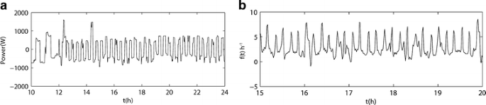

  

  a Alternating component of daily load curve (day 0). b Instantaneous frequency f(t) for the load curve shown in Fig. 11. For simplicity, f(t) is only shown from 15 to 20 h

• (b) Apply HT to the new load waveform, compute analytic signal and instantaneous frequency

  The second step is to evaluate H[g(t)] for each “centred” daily load curve (days 0–3) and then compute s(t) and f(t). As shown in Fig. 11, the frequency f(t) during the day is quite far from the frequency of an ideal rectangular wave (see Fig. 3). This is due to the presence of several square waves with their own switching ON/OFF pattern on the customer side. At any rate, some properties, e.g. the concavity/convexity, cycling and sharp peaks of f(t), in ideal curves appear again in real daily load curves.

• (c) Obtain the average frequency of the cycling loads (hour by hour) with the help of the ACF function

  For the 3 days selected, the average frequency has been computed according to the ACF values. Note that in the first iterations of the method, several T ₁ periods are possible in each time cycle (i.e. the load could change ON/OFF patterns, see Fig. 10), or when the load can be switched off as a result of a DR policy, a change in the customer behaviour, or a change in the temperature (i.e. some feedback from load models is needed). Figure 12 shows the average frequencies and the ACF values (lags). The overall data supplied by ACF are presented in Table 4.

  Fig. 12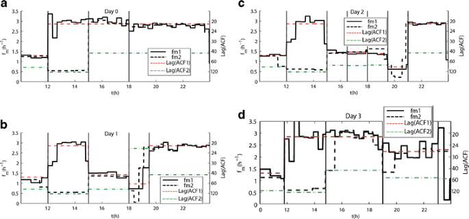

  

  Average frequency (f _m continuous and dashed black line) a day 0 (baseline), b day 1 (control), c day 2 (control) and d day 3 (control)

  Table 4 Time interval and filtered waveform characteristics

  As seen, in Table 4, positive ACF values are collected as lag in minutes for each hour interval (fourth column of this table). Some of them are just multiple of the main ACF value and represent the repetition of two and more cycles (for instance, 21 and 42). This is confirmed by the f _m calculation as the value remains the same for both coefficients (continuous and discontinuous black lines in Fig. 14 outside 12–15-h interval). However, other ACF values represent a second end use (component) of the load (signal). This is clearly seen on 12–15-h period, where two different frequencies are obtained (about 2.9 ON/OFF cycles/h continuous black line and about 0.6 cycles/h dashed black line) for each ACF.

• (d) Compute the amplitudes by using instantaneous amplitude A(t) evaluated with HT

  This step enables the aggregator to analyse which loads are cycling during the DR control period, verifying the magnitude of load changes and the credibility of load reduction for each customer.

  Figure 13 shows the amplitudes detected in the five time intervals of the day 2. The overall data have been collected in Table 4. The methodology is able to distinguish two cycling loads with similar demands, i.e. WH and EH (1,200 vs. 1,000 W, respectively). The average switching frequency f _m(t) and the cycling duty periods help the aggregator to distinguish each one.

  Fig. 13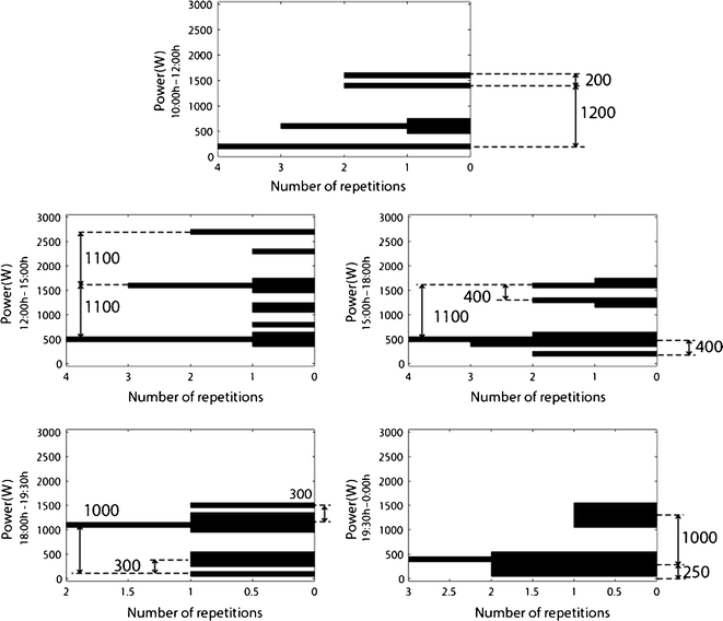

  

  Histogram of amplitudes for each zone detected in days 1 and 2

• (e) Determine the width of ON cycles to evaluate the reduction in energy due to DR policies

  In steps 3 and 4, the EH load is shown to be in use, and cycling ON/OFF, from 12 to 21 h. In the window enabled for DR purposes, for instance, due to the forecast of high-price periods in some windows (Gabaldón et al. 2010), the load is used with a lower duty cycle. This suggests the aggregator that an effective load change is being applied by its customer. Nevertheless, the results of DR policies (for instance, days 1 and 2) in demand have to be studied more accurately. In this case, according to the results presented in Table 3, the load under control had the same frequency in the control period (around 1.5 cycles/h), but in day 2, the load switched on with two different widths of ON pulse (i.e. the demand changes along the control period). Negative ACF values (sixth column in Table 4) are useful to determine the pulse width of the main component. Thus, another interesting characteristic of the load being controlled can be extracted easily. As seen in Table 4, the pulse width varies according to the DR load control (Fig. 10). Moreover, the “payback period” for each day can be determined using the data in Table 4 (around 50 min for day 1 and 70 min for day 2).

About the effects of sampling frequency

Sampling frequency f _s allows HT and the tool, in general, to have a better performance. The f _s used by our smart meter was of one sample per minute, which corresponds to a f _s of 60 h⁻¹. The minimum frequency value to define an oscillation needs at least five samples per cycle (Huang et al. 1998). As the cycling frequencies that are required to be detected are not more than 3 h⁻¹, at least five samples each 20s are needed (one sample each 5 s), which makes the minimum f _s needed theoretically 12 h⁻¹. Moreover, the ACF for the width pulse detection requires at least two samples per pulse. Thus, that makes necessary at least 12 h⁻¹ as f _s. However, the first of the previous statement does not work well for square/shapes in the case of frequency detection, and simulation demonstrates that at least 10 samples are needed per cycle, in our case 24 h⁻¹.

Figure 14 shows the ACF value for the time period 18–24 h of day 0 with an f _s of 12 and 24 h⁻¹. As it can be seen, the results are similar to the results obtained in Table 4 in the second case.

Fig. 14

Sampling frequency comparison. ACF coefficients for day 0 from 18 to 16 h with: a f _s = 12 h⁻¹ and c f _s = 24 h⁻¹. Average frequencies using the ACF coefficients: b f _s = 12 h⁻¹, d f _s = 24 h⁻¹. t _ON times are correctly extracted (2 × 5 min = 10 min and 5 × 2.5 min = 10 min) in both cases. However, only the second case provides accurate frequency computation

DR evaluation

The change in the demand due to DR policies, ΔE, can be computed with the help of the expression in Eq. 16:

$$ \begin{array}{c}\hfill \varDelta E={\displaystyle \underset{t_{\mathrm{start}}}{\overset{t_{\mathrm{end}}}{\int }}\left[\overline{m(t)}-\overline{u(t)}\right]{P}_{\mathrm{rat}}\mathrm{d}t}+{\displaystyle \underset{t_{\mathrm{end}}}{\overset{t_{\mathrm{payback}}}{\int }}\left[\overline{m(t)}-\overline{u(t)}\right]{P}_{\mathrm{rat}}\mathrm{d}t}\hfill \\ {}\hfill \overline{m(t)}=\frac{t_{\mathrm{ON}}(t)}{t_{\mathrm{ON}}(t)+{t}_{\mathrm{OFF}}(t)};{t}_{\mathrm{start}}<t<{t}_{\mathrm{payback}};\mathrm{day}\;0\hfill \\ {}\hfill \overline{u(t)}=\frac{t_{\mathrm{ON}}(t)}{t_{\mathrm{ON}}(t)+{t}_{\mathrm{OFF}}(t)};{t}_{\mathrm{start}}<t<{t}_{\mathrm{payback}};\mathrm{day}\mathrm{s}\;1\;\mathrm{and}\;2\hfill \end{array} $$

(16)

where:

m(t), u(t):

operational state without control and forced state under DR (natural and forced duty cycles).

t _ON, t _OFF :

pulse width in ON and OFF states, both vary in time.

P _rat :

rated power of the load being controlled.

t _start, t _end :

initial and final window times of the DR policy.

t _payback :

energy recovery time when the control period is over.

If the customer load is working in the DR control period together with a homogeneous control group for aggregation purposes, i.e. an ensemble of n loads with similar control and characteristics to obtain a minimum load level to participate in DR policies (usually about 100 kW of load reduction in east coast USA markets), the power change of this group in each DR interval is done by Eq. 17:

$$ \varDelta P=\left[\overline{m(t)}-\overline{u(t)}\right]n{P}_{\mathrm{rat}} $$

(17)

Using the mean frequencies f _m(t) and periods T ₁(t) of the main (or secondary) component, the average of the operational state m(t) and control state average u(t) can be obtained as Eq. 18:

$$ \overline{m(t)},\overline{u(t)}=\frac{t_{\mathrm{ON}}(t)}{t_{\mathrm{ON}}(t)+{t}_{\mathrm{OFF}}(t)}=\frac{t_{\mathrm{ON}}(t)}{T_1(t)}=\frac{t_{\mathrm{ON}}(t)}{60}{f}_m(t) $$

(18)

Note that each magnitude is computed in its corresponding period and day. Figure 15 presents the results of these equations, for the data given in Table 4, for an hypothetic control group of similar characteristics, which are being managed by the aggregator (size, around 1,000 customers). A more valuable information for the aggregator (customer comfort, the effect of climate parameters) should need the use of HT and physically based load models as a whole (Gabaldón et al. 2010).

Fig. 15

Energy behaviour of EH load during and after the control period. The control period is applied from 14 to 21 h

The results of the proposed method for load disaggregation and the evaluation of load response when DR is applied are presented in Table 5 (for the individual customer and end uses shown in Table 1, and excluding the payback period). For testing purposes, the real end-use data (Figs. 1 and 9) for each control day are considered, too. The results show that the proposed method has proved to be reasonably accurate. Note that this accuracy is apparently low because rated power of EH has been overestimated in some periods (see Fig. 13, Tables 2 and 4, in the time period from 15 to 18 h).

Table 5 Energy results: real and estimated for the individual customer

Energy efficiency

Another concern for both the aggregator and the customer is efficiency in energy and costs. The efficiency in cost, cost management, is of interest, too (Goldman et al. 2010). In this case, the disaggregation of water heater (through the inverse Hilbert transform and the data of Table 4) is shown in Fig. 16. Note that the end use is extracted with a good accuracy (disaggregated WH demand of 5.34 kWh/day vs. actual demand of 5.1 kWh/day), but some minor error is present (see arrows in this Fig. 16). This customer behaviour gives the aggregator: First, the possibility to offer specific information to its customer, and then the possibility to evaluate with more precision the cost effectiveness of well-known policies, for example, a change in the customer tariff or the upgrade of WH to more efficient technologies (heat pump water heater) or the change of WH to other with a higher capacity to provide full storage. Moreover, for the new capacity markets being developed in the USA (Jenkins et al. 2011), the mining of these end-use patterns allow a more precise evaluation of energy offers.

Fig. 16

Energy behaviour of WH and EH loads under the three cases studied (recorded dashed line; estimation solid line). Arrows show errors in the disaggregation of the end use

Conclusions

This paper presents an alternative method for load disaggregation of end uses with cycling demand. The tool developed allows extracting important information of loads in normal use and loads being controlled to verify DR performance (power level, cycling frequency and width pulse). The method proposed demonstrates that HT properties can still be used not only to analyse rectangular waveforms but also to estimate the cycling frequency of the major component of complex (multi-component) signals. These properties of the integral transform and the use of statistical tools (applied in the domain of transform), such as autocorrelation function, provides the information needed to the end-use disaggregation: the level of demand and the duty cycles of the end use. This information can be of the greatest interest for the data supplied by the future deployment of AMI technologies. These data will be readily available in the near future thanks to the EU and USA policies made to promote the establishment of advanced metering technologies in all the customer segments. Hence, the information obtained (load curves) is “filtered” to determine the natural and forced cycles for high demand end uses at households. This allows the demand aggregator to identify the potential of main end uses (efficiency and demand response policies) and, besides, verify and evaluate the response of selected (representative) customers in each demand segment and, in this way, to obtain the maximum potential available out of DR and EE.

References

Almeida, A. T. de, & Fonseca, P. (2010). Residential monitoring to decrease energy use and carbon emissions in Europe. EACI-Intelligent Energy Europe project report, 2006–2008, ISR-University of Coimbra.
Bertoldi, P., Hirl, B., Labianca, N. Energy efficiency status report. Joint Research Centre, 2012. http://iet.jrc.ec.europa.eu/energyefficiency/sites/energyefficiency/files/energy-efficiency-status-report-2012.pdf. Accessed 2 May 2013.
Box, G. E. P., Jenkins, G. M., & Reinsel, G. C. (1994). Time series analysis: Forecasting and control (3rd ed.). Upper Saddle River: Prentice-Hall.
Browne, T. J., Vittal, V., Heydt, G. T., & Messina, A. R. (2008). A comparative assessment of two techniques for modal identification from power system measurements. IEEE Transactions on Power Systems, 23(3), 1408–1415.
Chang, H. H. (2012). Non-intrusive demand monitoring and load identification for energy management systems based on transient feature analyses. Energies, 5, 4569–4589.
Deering, R., & Kaiser, J. F. (2005). The use of a masking signal to improve empirical mode decomposition. Proceedings of IEEE International Conference on Acoustics, Speech, and Signal Processing, 4, 485–488.
EIA. (2001). End-use consumption electricity 2001. http://www.eia.gov/emeu/recs/recs2001/enduse2001/enduse2001.html. Accessed 2 May 2013.
Elliott, R. J., Aggoun, L., & Moore, J. B. (1995). Hidden Markov models. New York: Springer Science+Business Media.
Johnson Controls. (2010). Energy performance contracting in the European Union: Introduction, barriers and prospects. Milwaukee: Johnson Controls.
European Commission. (2011). Energy efficiency plan 2011, COM (2011) 109 final. http://eur-lex.europa.eu/LexUriServ/LexUriServ.do?uri=COM:2011:0109:FIN:EN:PDF. Accessed 4 Feb 2013.
European Parliament and Council. Directive 2012/27/EU of the European Parliament and of the council of October 2012 on energy efficiency, amending directives 2009/125/EC and 2010/30/EU. http://eur-lex.europa.eu/LexUriServ/LexUriServ.do?uri=OJ:L:2012:315:0001:0056:EN:PDF. Accessed Nov 2013.
Faruqui, A., Harris, D., & Hledick, R. (2010). Unlocking the €53 Billion Savings from Smart Meters in the EU: How increasing the adoption of dynamic tariffs could make or break the EU’s smart grid investment. Energy Policy, 38(10), 6222–6231.
Faruqui, A., Sergici, S., & Akaba, L. (2013). Dynamic pricing of electricity for residential customers: The evidence from Michigan. Energy Efficiency, 6, 571–584.
Gabaldón, A., Guillamón, A., Ruiz, M. C., Valero, S., Ortiz, M., & Alvarez, C. (2010). Development of a methodology for clustering electricity-price series to improve customer response initiatives. IET Generation, Transmission & Distribution, 4(6), 706–715.
Goldman, Ch., Reid, M., Levy, R., Silverstein, A. (2010). Coordination of energy efficiency and demand response, LBNL report 3044E.
Gomatom, K., & Homes, C. Evaluation of NILMs technologies for electric load disaggregation. 1st International Workshop on Non-Intrusive Load Monitoring, Pittsburgh, PA, USA, May 2012.
Greenbang. (2012). Europe’s smart meter outlook for 2020 a $25 billion market. http://www.greenbang.com/wp-content/uploads/2012/02/Smart-Meter-Outlook-2020.pdf. Accessed 15 Oct 2013.
Hart, G. W. (1992). Nonintrusive appliance load monitoring. Proceedings of the IEEE, 80(12), 1870–1891.
Huang, N. E., Shen, Z., Long, S. R., & Manli, C. W. (1998). The empirical mode decomposition and the Hilbert spectrum for nonlinear and nonstationary time series analysis. Procedures of the Royal Society of London, 454(1971), 903–995.
Jenkins, C., Neme, C., & Enterline, S. (2011). Energy efficiency as a resource in the ISO New England capacity market. Energy Efficiency, 4(1), 31–42.
Kim, H., Marwah, M., Arlitt, M., Lyon, G., Han, J. (2011). Unsupervised disaggregation of low frequency power measurements. Proceedings of the 11th SIAM Conference on Data Mining (pp. 747–758). Arizona: USA.
Kolter, J. Z., & Johnson, M. J. (2011). REDD: A public data set for energy disaggregation research. Proceedings of the SustKDD workshop on Data Mining Applications in Sustainability. San Diego, CA, USA.
Koponen, P. (2012). Measurements and models of electricity demand responses. Research Report VTT-R-09198-11, VTT 2012. http://www.cleen.fi/en/sgem/public_deliverables#Technical. Accessed 2 May 2013.
Liang, J., Simon, K., Kendall, G., & Cheng, J. (2010a). Load signature study. Part I: basic concept, structure and methodology. IEEE Transactions on Power Delivery, 25(2), 551–560.
Liang, J., Simon, K., Kendall, G., & Cheng, J. (2010b). Load signature study. Part II: Disaggregation framework, simulation, and applications. IEEE Transactions on Power Delivery, 25(2), 561–569.
Piette, M. A., Watson, D., Motegi, N., Kiliccote, S. (Lawrence Berkeley National Laboratory). (2007). Automated critical peak pricing field tests: 2006 pilot program description and results. California Energy Commission, PIER Energy Systems Integration Research, Program. CEC-500-03-026, 2007.
Poularikas, A. D. (1999). The handbook of formulas and tables for signal processing. Boca Raton: CRC.
Senroy, N., Suryanarayanan, S., & Ribeiro, P. F. (2007). An improved Hilbert–Huang method for analysis of time-varying waveforms in power quality. IEEE Transactions on Power Systems, 22(4), 1843–1850.
Zeifman, M., & Roth, K. (2011). Nonintrusive appliance load monitoring: Review and outlook. IEEE Transactions on Consumer Electronics, 57(1), 76–84.
Acknowledgements
This work was supported by the Spanish Government (Ministerio de Economía y Competitividad) and EU-FEDER funds under Research Project ENE2010-20495-C02-02.
Author information
Authors and Affiliations
Corresponding author
Rights and permissions
Open Access This article is distributed under the terms of the Creative Commons Attribution 2.0 International License ( https://creativecommons.org/licenses/by/2.0 ), which permits unrestricted use, distribution, and reproduction in any medium, provided the original work is properly cited.
About this article
Cite this article
Gabaldón, A., Ortiz-García, M., Molina, R. et al. Disaggregation of the electric loads of small customers through the application of the Hilbert transform. Energy Efficiency 7, 711–728 (2014). https://doi.org/10.1007/s12053-013-9250-6
Received:
Accepted:
Published:
Issue Date:
DOI: https://doi.org/10.1007/s12053-013-9250-6