
Abstract
State of the art travel demand models for urban areas typically distinguish four or five main modes: walking, cycling, public transport and car. The mode car can be further split into car-driver and car-passenger. As the importance of ridesharing may increase in the coming years, ridesharing should be addressed as an additional sub or main mode in travel demand modeling. This requires an algorithm for matching the trips of suppliers (typically car drivers) and demanders (travelers of non-car modes). The paper presents a matching algorithm, which can be integrated in existing travel demand models. The algorithm works likewise with integer demand, which is typical for agent-based microscopic models, and with non-integer demand occurring in travel demand matrices of a macroscopic model. The algorithm compares two path sets of suppliers and demanders. The representation of a path in the road network is reduced from a sequence of links to a sequence of zones. The zones act as a buffer along the path, where demanders can be picked up. The travel demand model of the Stuttgart Region serves as an application example. The study estimates that the entire travel demand of all motorized modes in the Stuttgart Region could be transported by 7% of the current car fleet with 65% of the current vehicle distance traveled, if all travelers were willing to either use ridesharing vehicles with 6 seats or traditional rail.
Introduction
In ridesharing, a car driver (supplier) offers other travelers (demanders) the possibility to join the trip for a certain fee. The offered trip results solely from the individual need of the supplier to perform a particular movement. The supplier determines the main characteristics of the trip: origin, destination, departure time and choice of route. A ridesharing potential occurs, if the temporal and spatial trip characteristics of supplier and demander match. A ridesharing trip is generated if the demander accepts the offer of the supplier. While the supplier receives a certain cost compensation, the demander receives a convenient trip to the desired destination. Traditional ridesharing, also called carpooling, has the following characteristics:
-
The suppliers conduct their trips independently of any additional demand for a ride.
-
In the past, where only a small number of trips were on offer, ridesharing made sense only for long-distance trips (arranged by ridesharing agencies) or for regular trips (trip sharing with work mates).
New online platforms ensure the matching of suppliers and potential demanders at short notice. This dynamic ridesharing has become an option in short-distance transport offering an alternative for trips with no or inadequate public transport. In such cases, ridesharing can reduce car trips and contribute to a more sustainable transport. As the example of transport network companies (TNC) like Uber and Lyft shows, ridesharing can also be provided as a professional service offering taxi-like rideselling services, which may increase the number of car trips.
The expectation, that the importance of ridesharing will increase, be it in the form of carpooling or rideselling, requires transport planners to estimate the impacts of ridesharing. How big is the potential of ridesharing? What is the critical mass of suppliers necessary to ensure that demanders are offered a suitable trip with a high probability and short waiting times? What would happen, if fleets of self-driving cars offer ridesharing services? In order to find answers to these questions travel demand models may be helpful, if they are extended by an algorithm for the matching of offered and demanded trips.
This paper presents an algorithm for the matching of trips. It can be integrated in existing macroscopic travel demand models, which differ from microscopic travel demand models in several aspects (Table 1). The algorithm is based on the following assumptions:
-
Origin and destination of all trips of suppliers and demanders are located in traffic zones. Every trip originates in an origin zone, traverses a sequence of traffic zones along a shortest path until it terminates in the destination zone. Trips are only matched if their origin and destination lie within the sequence of the traversed zones. Suppliers will only make detours for picking up or dropping off passengers in the zones along the shortest path.
-
A traffic zone does not represent an exact meeting point for suppliers and demanders but it defines an appropriate area for this meeting. It is assumed that suppliers and demanders can arrange an appropriate meeting point within a zone. The exact meeting point, however, is not modeled. Longer trip times resulting from detours for picking up or dropping off demanders can be included by extra times depending on the size of the corresponding traffic zone.
-
The daily travel demand is available as a set of time-dependent demand matrices. The algorithm matches the trips for every matrix independently.
The paper does not address methods for determining the modal share of ridesharing trips within a travel demand model. The share can be set as an assumption (“assume 10% of all car drivers offer rides and 20% of all public transport users would take suitable offers”) or determined as an independent mode in the mode choice step of the travel demand model. In addition to traditional ridesharing with suppliers and demanders, the paper also addresses a case where individual suppliers are replaced by fleets of taxis or taxi-robots. This case permits to calculate the vehicle occupancy rates of such taxi fleets.
State of the art
Characteristics and perspective of ridesharing
De Marco et al. (2015) define dynamic ridesharing as “a system that facilitates the ability of drivers and passengers to make one-time ride matches close to their departure time, with sufficient convenience and flexibility to be used on a daily basis”. Another definition for a dynamic ridesharing is formulated by Agatz et al. (2011) as “a system where an automated process employed by a ride-share provider matches up drivers and riders on very short notice, which can range from a few minutes to a few hours before departure time”. Levofsky and Greenberg (2001) note that “dynamic ridesharing systems consider each trip individually and are designed to accommodate trips to random points at random times by matching user trips regardless of the trip purpose”. Agatz et al. (2012) describe the characteristics of a dynamic ridesharing concept. Some of the key features are:
-
Dynamic: mobile phones with internet access allow for matches on short-notice.
-
Cost-sharing: the variable costs of a trip are split between the rideshare participants.
-
Non-recurring trips: single-trip ridesharing does not require a rigid time schedule.
-
Automated matching: the ride matching should be automated to reduce the effort of the participants. The system finds suitable matches and facilitates the communication.
Uber Pool and Lyft Line prove that dynamic ridesharing works. The success indicates the potential of ridesharing. The current situation will change again with driverless cars. Statements of car manufacturers (Inventivio 2017) and scientific forecasts (Trommer et al. 2016; Litman et al. 2017; Bansal and Kockelman 2017) on the availability of self-driving cars still vary a lot, ranging from the near future to 2050 and beyond. Whenever the driverless car comes, it will open new business areas for mobility providers to offer mobility as a service including rideselling services.
The matching problem
The core of a ridesharing system is the trip matching process. The complexity of the matching problem depends on the number of trips. With an increasing number of trips, the number of possible matches increases. The challenge is to find reasonable solutions within a short computational time to run the system as an online real-time application.
The literature on the matching problem in ridesharing comprises various publications (for instance Baldacci et al. 2004; Calvo et al. 2004; Winter and Nittel 2006; Amey 2011; Di Febbraro et al. 2013) dealing with optimization aspects of rideshare problems including patents for the “Automated carpool matching” (Levine et al. 2010). While many approaches focus on fixed assigned demand, Kleiner et al. (2011) reformulate the optimization aspect as an adaptive dynamic ridesharing system that is capable to consider individual preferences of participants while matching the trips.
Ghoseiri et al. (2011) describe ridesharing systems operating in the US and formulate a “Dynamic Rideshare Matching Optimization Model”, introducing a wide range of additional marginal conditions (for instance gender). In addition, Shangyao and Chun-Ying (2011) consider different vehicle and person types to represent more closely the effects of real behavior aspects.
In travel demand modeling so far the ride matching problem is addressed exclusively in the context of microscopic demand modeling (for instance Shangyao and Chun-Ying 2011; Galland et al. 2013; Dubernet et al. 2013), in which the negotiation process of the transport users (agents) is modeled. Algorithms for matching non-integer demand, as it occurs in demand matrices of a macroscopic travel model, are not yet described to the knowledge of the authors.
Algorithm and implementation
An algorithm for solving the matching problem in an optimal way can for example aim at maximizing the number of matched trips or at maximizing the occupancy rate in the vehicles. The structure of the trip-matching problem is similar to the traveling salesman problem, which is a NP-hard optimization problem, if the optimal solution is required. To handle real world problem sizes with zone numbers over 1000 and trip numbers over 100,000 the algorithm presented in the following makes simplifications. The algorithm belongs to the class of greedy algorithms and therefore does not guarantee an optimal solution for the matching problem.
Input data
The algorithm requires supply and demand data as input. Supply data cover the nodes and links of the road network as it is required by a travel demand model. The supply data may specify selected nodes as locations for pick-up and drop-off. Demand data distinguish two types of demand matrices:
-
The demand matrix of the suppliers S. In a travel demand model they are a subset from the demand matrix of car-drivers, i.e. car drivers who are willing to provide a ride to unacquainted travelers not belonging to the family.
-
The demand matrix of the demanders D. In a travel demand model, they may come from a subset of the matrices for car-self driver, car-passenger and public transport users, who consider using a ridesharing service. They may also come from a specific ridesharing mode.
The demand should be available in small time intervals t (≤ 15 min) and in traffic zones of appropriate size (travel time in traffic zone ≪ average travel time of a trip). Thus St and Dt represent the demand matrices in time interval t.
Basic algorithm
The basic algorithm assumes that routes of the trips follow a shortest path and that every pick-up location belongs to exactly one traffic zone. With these limitations, the algorithm for matching the trips of one time interval consists of the following steps:
-
1.
Determining a set of reference objects for pick-up and drop-off locations A reference object describes the location in the network where potential ridesharers can be picked up. Reference objects can be road links, public transport stops or ridesharing meeting points. The basic algorithm described in the following assumes that the reference object is a link which refers to exactly one traffic zone z. Road links restricted to motor vehicles, where boarding is prohibited, should be excluded from the set of reference objects.
-
2.
Assigning a zone z to each link l Every link l of the road network is assigned to one or no zone number. The assignment requires an intersect operation as provided by Geographic Information Systems (see Fig. 1).
Fig. 1 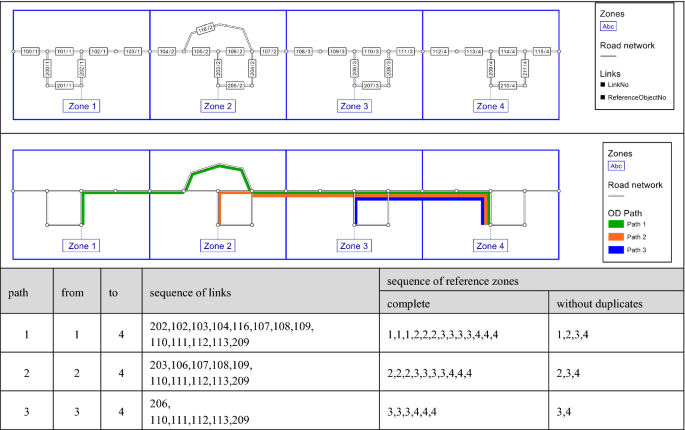
Preparation of paths for the matching procedure
-
3.
Determining two path sets P for suppliers and demanders For every time interval t the two demand matrices St and Dt are assigned to the transport network using a shortest-path assignment. The result is one path set for the suppliers P S t and one path set for the demanders P D t for every time interval t. Each set contains maximum one path p for each od-pair with the corresponding demand of the suppliers \( d_{p,t}^{S} \) and demanders d D p, t .
-
4.
Reducing paths from a sequence of links to a sequence of zones Each path of a path set \( p \in P_{t} \) traverses a sequence of links \( l_{1} ,l_{2} , \ldots ,l_{n} \) and in doing so, a sequence of zone objects \( z_{{l_{1} }} ,z_{{l_{2} }} , \ldots ,z_{{l_{n} }} \). The sequence of zone objects is stored as a string attribute of a path. It describes the sequence of traversed traffic zones where demanders can be collected. The sequence of zone objects often contains the same zone object several times (\( z_{{l_{1} }} \equiv z_{{l_{2} }} ) \). In this case, duplicate zone objects are deleted. As a result, each path is reduced to a sequence of zones containing considerably less elements than the sequence of links. Figure 1 illustrates the procedure to obtain a reduced sequence of zone objects.
-
5.
Assigning a capacity to each path of the suppliers Each path of the supplier path set \( P_{t}^{S} \) obtains a capacity resulting from the demand volume of the supplier and the average vehicle capacity (for instance a 5-seat-vehicle). As suppliers may travel with private car passengers, e.g. family members, the capacity needs to be reduced appropriately. Equation (1) shows how to compute the available capacity for ridesharing for one path including car passenger demand on od-level. Equation (2) determines the capacity using an average occupancy rate:
$$ c_{p,t}^{S} = c_{o,d,t}^{S} = (c^{veh} - 1) \cdot d_{o,d,t}^{S} - d_{o,d,t}^{CarPass} $$(1)$$ c_{p,t}^{S} = c_{o,d,t}^{S} = \left( {c^{veh} - o^{veh} } \right) \cdot d_{o,d,t}^{s} $$(2)where c S p, t capacity for ridesharing provided by supplier on path p in time interval t. In the case of a shortest path match, path capacity is equal to the capacity c S o, d, t from zone o to zone d; cveh average vehicle capacity including driver; d s o, d, t travel demand of suppliers from zone o to zone d in time interval t; d CarPass o, d, t travel demand of private car passengers from zone o to zone d in time interval t; oveh average occupany rate of a private car: oveh = (ds + dCarPass)/ds
Assuming a supplier demand of 0.2 car trips along a particular path, a car passenger demand of 0.06 and a vehicle capacity of 5 places, the available capacity for ridesharers is \( \left( {5 - 1} \right) \cdot 0.20 - 0.06 = 0.74 \) persons. In this calculation (5 − 1) = 4 represents the free capacity of one car with one driver. As it is a macroscopic model, the supplier demand of the path is non-integer. This leads to \( 4 \cdot 0.20 = 0.8 \) empty places on the path, out of which 0.06 places are already taken by car passengers traveling with the driver, e.g. family members.
-
6.
Matching of paths The matching of the two path sets P S t and P D t compares the reduced paths of zone sequences. A full match occurs, if the origin and destination zones of \( p^{D} \in P_{t}^{D} \) and \( p^{S} \in P_{t}^{S} \) are identical. A partial match occurs if path pD is covered by pS, i.e. pD ⊂ pS. Path pD is covered by path pS if origin o and destination d of path pD occur in the right order (o before d) in the zone sequence of path pS. This can be implemented as a string comparison. Figure 1 illustrates the advantage of matching paths not on the level of links but on the level of zones: This allows identifying paths, which are not completely identical, but still suitable for a match. The matching process starts with fully matching paths. The remaining paths are processed sequentially, starting with the first path of the path set P D t . There are other possibilities to process the remaining paths, for instance starting with the longest path.
-
7.
Reduction of path capacity and path demand After every match, the sharing capacity \( c_{{p^{S} ,t}}^{S} \) of path pS is reduced according to Eq. (3) by the demand of ridesharers moving along path pD ⊂ pS until the entire capacity is utilized. At the same time the unsatisfied ridesharing demand is reduced as shown in Eq. (4):
$$ c_{{p^{S} ,t}}^{S} = \left\{ {\begin{array}{*{20}l} {c_{{p^{S} ,t}}^{S} - d_{{p^{D} \subset p^{S} ,t}}^{D} } \hfill & {\quad if\; demand \; \le \;capacity} \hfill \\ 0 \hfill & {\quad if\; demand \; > \;capacity} \hfill \\ \end{array} } \right. $$(3)$$ d_{{p^{D} \subset p^{S} ,t}}^{D} = \left\{ {\begin{array}{*{20}l} 0 \hfill & {\quad if\, demand \, \le \,capacity} \hfill \\ {d_{{p^{D} \subset p^{S} ,t}}^{D} - c_{{p^{S} ,t}}^{S} } \hfill & {\quad if\, demand \, > \,capacity} \hfill \\ \end{array} } \right. $$(4) -
8.
Recording of unsatisfied demand After all paths of a time interval have been checked to identify matches, the number of demanders finding a match (satisfied ridesharing demand) and the number of demanders without a match (unsatisfied ridesharing demand) can be summed up over all paths. For every pick-up stop the travel time increases by a certain value. The additional travel time can be implemented as fixed value (e.g. 4 min for each stop) or as function of the boarding demand.

Extensions of the algorithm
The implementation of the described basic ridesharing algorithm can be extended in the following ways:
-
Handling rideselling systems This refers to a case where the suppliers are not private car drivers but taxi-like rideselling services with professional drivers or driverless cars. In this case, only the demand matrix of the demanders is used as input. In the matching step all paths of the path set P D t are compared to each other. Two paths p D1 and p D2 are matched if one of the two conditions hold: p D1 ⊂ p D2 or p D1 ⊃ p D2 . This approach assumes that the number of taxis is not limited.
-
Smart match A partial matching following the path order (i.e. matching the first supplier to the first demander path according to the order of the zone numbers) unnecessarily wastes unused ridesharing capacity. Instead, paths can be matched in such a way that either the paths with the longest shared distance or the paths with the highest demand are matched first.
-
Arbitrary reference objects referring to one zone The basic algorithm described above assumes that every link belongs to maximum one zone, as it is the case in Fig. 2 a. Figure 2 b presents a case, where the reference object is not a link but a dedicated ridesharing meeting point. This meeting point is assigned to exactly one zone. The unique zone number of the meeting point is then assigned to all links within a certain buffer around the meeting point. This buffer expresses the willingness of suppliers to accept detours for picking up and dropping off demanders. As a result, a link may belong to more than one zone. This leads to a modified sequence of zones, which can then be processed as in the basic algorithm.
Fig. 2 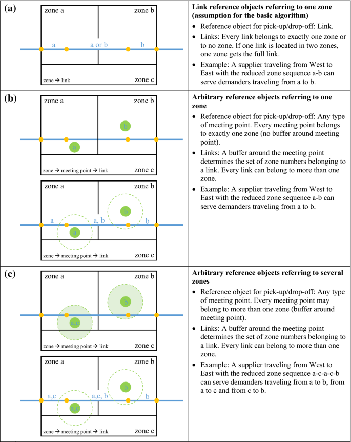
Methods for assigning zone numbers to links
-
Arbitrary reference objects referring to several zones Figure 2c presents a case where a meeting point can be linked to more than one zone. This case again may lead to a modified sequence of zones thus influencing the results.
-
Multi-path The shortest path assignment can be extended by any other multi-path assignment method leading to od-pairs with more than one path. In this case, the ridesharing capacity of the od-pair needs to be distributed to every path. One simple solution is to use the shares from the traffic assignment.

Implementation
The algorithm described above is implemented in the transport planning software of PTV VISUM (2017). VISUM contains all data structures of the transport supply (nodes and links) and of the travel demand (traffic zones, demand matrices). Of major importance for the matching are route objects that are saved in VISUM as the results of a traffic assignment. A route object p is made up of data describing the route (the demand on the particular route, length and travel time) and the route elements (sequence of nodes respectively links). Using the VISUM-route objects and the methods available in VISUM (e.g. intersecting and shortest-path assignment), a matching of routes can be implemented with less than 100 lines of code.
Computation time increases with the square of the number of paths, which are compared in the matching step. In order to reduce computation time, the search engine Elasticsearch (2017) is integrated into the processing sequence of VISUM using a Python script. The path sets of suppliers and demanders are handed over to the search engine. The result from the search process is a list with possible routes for the matching process. The matching part of the algorithm then decides which demanded route is assigned to one or several routes from the subset of supplied routes depending on capacity restrictions. Elasticsearch helped to reduce the computation time considerably by a factor of 1000.
For the two scenarios presented below a 64 GB RAM computer with an Intel(R) Core(TM) i7-5820 k 3.30 GHz processor required a computation time of approximately 1 h for scenario S1 (1100 zones, 96 time intervals, 300,000 demanders, 150,000 suppliers) and 3 h for scenario S2 (1100 zones, 96 time intervals, 1,200,000 demanders, 750,000 suppliers).
The Institute for Road and Transport Science (2017) provides a link to a toy network to demonstrate the ridesharing algorithm. The procedure is simplified with respect to the process how the algorithm detects paths that could be matched. Therefore, the procedure works without external libraries and is directly executable if VISUM 16 is installed on a local machine.
Results
The algorithm is applied to the Stuttgart Region (Schlaich and Analyseverkehr 2009), a polycentric region with 2.7 million inhabitants living in several towns, but also rural areas. On a workday, the inhabitants produce roughly 5 million motorized trips, out of which 3 million are car-drivers, 1 million are car-passengers and 1 million use public transport. This travel demand is replicated in a travel demand model with 1100 traffic zones distinguishing 23 person groups and 19 trip purposes. The demand is available for 96 time intervals of 15 min each. Although the algorithm is suitable for handling non-integer demand matrices, the experiments described below apply integer demand matrices, i.e. full trips.
Until now, there is little information to what extent travelers would participate in an area-wide short-distance ridesharing, be it as supplier or as demander. Thus instead of applying a utility-based mode choice model, the example calculations use assumptions for the following modal shares:
-
Share of car-drivers willing to offer rides (supplier),
-
Share of car-drivers willing to take a ride and leaving their own vehicle at home (demander),
-
Share of public transport users willing to shift from public transport (demander).
For estimating the ridesharing potential of the Stuttgart Region, two scenarios with the following characteristics are analyzed assuming a passenger car with 5 seats:
-
S1: 5% of the car-drivers are willing to offer a ride. The remaining 95% use their vehicle as before. 25% of the public transport users are prepared to shift to ridesharing alternatives, if a match is provided.
-
S2: 25% of the car-drivers are willing to offer a ride. Further 5% of the car-drivers would shift to ridesharing if a match is available. The remaining 70% use their vehicles as they did before. All public transport users (100%) are willing to shift to ridesharing.
Figure 3 shows the results for scenario S1 and Fig. 4 for scenario S2. The red graph displays the trips of the suppliers, the blue graph the trips of the demanders. The green graph indicates the satisfied demand of the demanders. The matching rate depends on the number of suppliers and demanders: the higher the number of suppliers, the higher the probability that a ridesharing request can be served, thus increasing the attractiveness of the system.

S1: Ridesharing potential during the course of a working day if 5% of the car-drivers serve as suppliers and 25% of the public transport users act as demanders

S2: Ridesharing potential during the course of a working day if 25% of the car-drivers serve as suppliers and 100% of the public transport users along with 5% of the car-drivers act as demanders
During an entire day, 13% of all ridesharing requests can be served in scenario S1, and 28% in scenario S2. The probability to find a match between 8:00 and 18:00 is in both scenarios higher than in the other hours. This has two reasons: (1) During the early and late hours of a day the demand is low, making it harder to find a match. (2) The share of users traveling during the morning peak is higher in public transport compared to private car transport, mainly because of school trips. This leads to a lower ratio of supplied and demanded trips between 6:00 and 8:00 compared to other hours. Ridesharing can obviously not cover school trips shifting from public transport to ridesharing. The comparison of scenario S1 and S2 illustrates the importance of a critical mass of participants to make a ridesharing system operational. Both sides profit from a high number of participants. Demanders obtain a higher reliability and suppliers will be able to reduce their trip costs by picking up demanders.
Another indicator beside the share of matched trips is the vehicle occupancy rate. If a supplier does not find a matching request, the occupancy rate is 1.0. Figure 5 shows the occupancy rate of scenario S2 during the course of a day. It ranges from vehicles with one person (dark color) to vehicles with all seats occupied (light color). Low occupancy rates occur primarily during times with low demand early in the morning and late in the evening or in low-density areas away from central network axes. The average occupancy rate is 2.5, which is approximately twice the current occupancy rate.

Vehicle occupancy rate during the course of the day
Conclusion and outlook
State of the art travel demand models for urban areas typically distinguish four or five main modes: walking, cycling, public transport and car. The mode car can be further split into car-driver and car-passenger. As the importance of ridesharing may increase in the coming years, ridesharing should be addressed as an additional main mode or sub mode in travel demand modeling:
-
Ridesharing as sub mode: This seems appropriate for traditional ridesharing systems, i.e. systems where drivers offer rides for journeys they are conducting as part of their daily travel pattern. In this case, ridesharing supplements public transport. Using such a system demanders cannot rely on the service and they need a backup mode, which is usually public transport. In a travel demand model the modal share of ridesharing would therefore be determined after the normal mode choice between the main modes within the public transport assignment.
-
Ridesharing as main mode: This seems appropriate for rideselling systems with professional drivers or driverless cars providing an on-demand shared taxi system. In this case, ridesharing competes with car and public transport. In such a system, it is less likely that demanders would need a backup mode. The modal share of ridesharing would be determined as an additional main mode in the normal mode choice step of the travel demand model. It would compete with car and public transport.
Both cases require an algorithm for matching the trips of suppliers (private car drivers or professional taxis) and demanders (travelers not using private cars). The algorithm described above offers a straightforward solution for the matching problem, as it simplifies the matching problem in several ways:
-
1.
Traffic zones serve as origins and destinations, precise pick-up/drop-off locations are not modeled.
-
2.
The representation of a path in the road network is reduced from a sequence of links to a sequence of zones. The zones act as a buffer along the path, where demanders can be picked up.
-
3.
The temporal distribution of demand is not continuous but uses time intervals.
These simplifications have advantages and disadvantages, which are summarized in Table 2.
The authors developed the algorithm for a study, which analyzed the impacts of large ridesharing systems with driverless cars on the number of required vehicles and the vehicle distance traveled. Similar to a study for Lisbon (OECD 2015), the study (Friedrich 2016; Friedrich et al. 2017) estimated that the entire travel demand of all motorized modes in the Stuttgart Region could be transported by 7% of the current car fleet with 65% of the current vehicle distance traveled, if all travelers were willing to either use ridesharing vehicles with 6 seats or traditional rail. Estimating the number of cars for such a system requires a vehicle-blocking algorithm, which assigns every ridesharing trip to one specific car. In the study, an algorithm working with integer demand was applied to determine the number of vehicles and the empty trips between drop-off and pick-up locations. The authors are currently working on a blocking algorithm working with non-integer demand using algorithms from doubly constrained trip distribution models. Only then, rideselling systems with professional drivers or self-driving cars can be fully integrated in traditional macroscopic travel demand models.
References
Agatz, N.A., Erera, A.L., Savelsbergh, M.W., Wang, X.: Dynamic ride-sharing: a simulation study in metro Atlanta. Transportation Research Part B: Methodological 45(9), 1450–1464 (2011). https://doi.org/10.1016/j.trb.2011.05.017
Agatz, N., Erera, A., Savelsbergh, M., Wang, X.: Optimization for Dynamic Ride-Sharing: a review. Eur. J. Oper. Res. 223(2), 295–303 (2012). https://doi.org/10.1016/j.ejor.2012.05.028
Amey, A. Proposed Methodology for Estimating Rideshare Viability Within an Organization: Application to the MIT Community, 90th Annual Meeting of the Transportation Research Board, vol. 11-2585, 2011
Baldacci, R., Maniezzo, V., Mingozzi, A.: An exact method for the car pooling problem based on lagrangean column generation. Oper. Res. 52(3), 422–439 (2004). https://doi.org/10.1287/opre.1030.0106
Bansal, P., Kockelman, K.M.: Forecasting Americans’ long-term adoption of connected and autonomous vehicle technologies. Transportation Research Part A: Policy and Practice 95, 49–63 (2017). https://doi.org/10.1016/j.tra.2016.10.013
Calvo, R.W., de Luigi, F., Haastrup, P., Maniezzo, V.: A distributed geographic information system for the daily car pooling problem. Comput. Oper. Res. 31(13), 2263–2278 (2004). https://doi.org/10.1016/S0305-0548(03)00186-2
De Marco, A., Giannantonio, R., Zenezini, G.: The diffusion mechanisms of dynamic ridesharing services. Prog. Ind. Ecol., 9(4), 408–432. ISSN 1476-8917 (2015). https://doi.org/10.1504/pie.2015.076900
DFG—Forschergruppe 2083: Integrierte Planung im öffentlichen Verkehr (Integrated planning in public transport). https://for2083.math.uni-goettingen.de/. Accessed 20 May 20 2018
Di Febbraro, A., Gattorna, E., Sacco, N.: Optimization on dynamic ridesharing systems. Transp. Res. Rec. J. Transp. Res. Board 2359, 44–50 (2013). https://doi.org/10.3141/2359-06
Dubernet, T., Rieser-Schüssler, N., Axhausen, K.W.: Using a multi-agent simulation tool to estimate the carpooling potential. In: 92th Annual Meeting of the Transportation Research Board, vol. 13-0866 (2013). https://doi.org/10.3929/ethz-b-000052402
Elastic. www.elastic.co. Accessed 20 July 2017
Friedrich, M., Hartl, M.: MEGAFON—modellergebnisse geteilter autonomer Fahrzeugflotten des öffentlichen Nahverkehrs, Schlussbericht, gefördert von: Ministerium für Verkehr Baden-Württemberg, Verband Deutscher Verkehrsunternehmen e. V., Stuttgarter Straßenbahnen AG, Verkehrs- und Tarifverbund Stuttgart GmbH, 2016. https://www.vdv.de/megafon-abschlussbericht-20161212.pdfx. Accessed 20 July 2017
Friedrich, M., Hartl, M., Magg, C.: Modelling vehicle sharing with driverless cars, conference simulation science, Göttingen (2017). http://www.simscience2017.uni-goettingen.de/wp-content/uploads/2018/01/SimScienceWorkshop2017_final.pdf, Accessed 20 July 20 2017
Galland, S., Gaud, N., Knapen, L., Janssens, D., Lamotte, O.: Simulation model of carpooling with the janus multiagent platform. Procedia Comput. Sci. 19, 860–866 (2013). https://doi.org/10.1016/j.procs.2013.06.115
Ghoseiri, K., Haghani, A.E., Hamedi, M.: Real-time rideshare matching problem. Mid-Atlantic Universities Transportation Center (2011). http://www.mautc.psu.edu/docs/UMD-2009-05.pdf. Accessed 20 July 2017
Institute for Road and Transport Science, Ridesharing Tool. www.isv.uni-stuttgart.de/vuv/tools/ridesharing/index.html. Accessed 20 July 2017
Inventivio. Driverless car market watch—Forecasts. Available at http://www.driverless-future.com/?page_id=384. Accessed 20 July 2017
Kleiner, A., Nebel, B., Ziparo, V.: A mechanism for dynamic ride sharing based on parallel auctions. In: Proceedings of the 22th International Joint Conference on Artificial Intelligence (IJCAI), Barcelona, Spain, pp. 266–272 (2011). https://doi.org/10.5591/978-1-57735-516-8/ijcai11-055. ISBN 978-1-57735-516-8
Levine, U., Shinar, A., Shabtai, E., Shmuelevitz, Y.: Automated carpool matching, U.S. Patent Application No. 12/453,133, 2010
Levofsky, A., Greenberg, A.: Organized dynamic ride sharing: the potential environmental benefits and the opportunity for advancing the concept. In: 92th Annual Meeting of the Transportation Research Board, vol. 01-0577 (2001). http://ridesharechoices.scripts.mit.edu/home/wp-content/papers/GreenburgLevofsky-OrganizedDynamicRidesharing.pdf. Accessed 20 July 2017
Litman, T.: Autonomous vehicle implementation predictions, victoria transport policy (2017). https://www.vtpi.org/avip.pdf. Accessed 20 July 2017
OECD, International Transport Forum. Urban mobility system upgrade. How shared self-driving cars could change city traffic (2015). https://www.itf-oecd.org/sites/default/files/docs/15cpb_self-drivingcars.pdf. Accessed 20 July 2017
PTV VISUM. http://vision-traffic.ptvgroup.com/en-us/products/ptv-visum/. Accessed 20 July 2017
Schlaich, J.: Verkehrsmodellierung für die Region Stuttgart. Analyseverkehr 2009/2010. Schlussbericht Modellierung. Karlsruhe (2011)
Shangyao, Y., Chun-Ying, C.: An optimization model and a solution algorithm for the many-to-many car pooling problem (2011). https://doi.org/10.1007/s10479-011-0948-6
Trommer, S., Koarova, V., Fraedrich, E., Kröger, L., Kickhöfer, B., Kuhnimhof, T., Lenz, B., Phleps, P.: Ifmo, autonomous driving—the impact of vehicle automation on mobility behaviour (2016). https://www.bmwgroup.com/content/dam/bmw-group-websites/bmwgroup_com/company/downloads/de/2016/Dezember%202016.pdf. Accessed 20 July 2017
Winter, S., Nittel, S.: Ad hoc shared-ride trip planning by mobile geosensor networks. Int. J. Geogr. Inf. Sci. 20(8), 899–916 (2006). https://doi.org/10.1080/13658810600816664
Acknowledgements
This research was funded by Deutsche Forschungsgemeinschaft (DFG, German Research Foundation) as part of the research group for integrated planning in public transport (DFG 2018).
Author information
Authors and Affiliations
Contributions
M. Friedrich developed the conceptual idea and the formal definitions. M. Hartl implemented the algorithm and performed the data analysis. C. Magg prepared the input data. All authors reviewed the literature, contributed to the development of the algorithm, discussed the results and drafted the manuscript. All authors read and approved the final manuscript.
Corresponding author
Rights and permissions
Open Access This article is distributed under the terms of the Creative Commons Attribution 4.0 International License (http://creativecommons.org/licenses/by/4.0/), which permits unrestricted use, distribution, and reproduction in any medium, provided you give appropriate credit to the original author(s) and the source, provide a link to the Creative Commons license, and indicate if changes were made.
About this article

Cite this article
Friedrich, M., Hartl, M. & Magg, C. A modeling approach for matching ridesharing trips within macroscopic travel demand models. Transportation 45, 1639–1653 (2018). https://doi.org/10.1007/s11116-018-9957-5
Published:
Issue Date:
DOI: https://doi.org/10.1007/s11116-018-9957-5