
Abstract
The problem of feedback control of mechanisms with joint clearance is analysed. Various control strategies are reviewed: impactless trajectories with persistent contact, control through collisions, the stabilization of equilibrium points, and trajectory tracking control. This article sets a general control framework, brings some preliminary answers and leaves some problems open, which are mentioned throughout the article and in the conclusions.
1 Introduction
Lagrangian mechanical systems subject to unilateral constraints, impacts and friction, make a rich class of nonsmooth, nonlinear dynamical systems. Though a lot remains to be discovered, it seems that constrained manipulators, biped robots, kinematic chains with joint clearance, juggling systems, tensegrity (cable-driven) and tethered systems, etc., possess different stability and control properties. It is therefore necessary to analyse the control of each subclass separately. Within the framework of multi-rigid-body systems with joint clearance, the main modelling issue concerns the choice of the contact model. Clearances involve additional degrees of freedom and introduce unilateral constraints. There are several available classes of models for collisions between bodies in the Mechanical Engineering literature; see, e.g. [14, Chaps. 2, 4, 5, 6] and [25, Chap. 3]. Commonly used two-body impact models in the Multibody System’s literature are extensions of Hertzian contact with added dissipation, the most well-known being the Simon–Hunt–Crossley and the Kuwabara–Kono dissipations, as well as their many variants like bistiffness Lankarani–Nikravesh and Walton–Braun models [14, §2.2.2, §4.2.1.2]. The main issue is that clearances may involve conformal contacting surfaces, which do not satisfy basic requirements for Hertzian elasticity (see [61, Table 2] for plane/plane contact elasticity coefficient). Moreover, the dissipation modelling is also a tough issue, and it is not clear whether or not nonlinear viscosity may be a suitable model. An advantage of compliant models is that they allow for the contact force history computation; however, this is not necessarily of interest for the design of feedback controllers, especially if the impact duration \(t_{f}\) is very short and prevents the actuators from being active during collisions (linear spring–dashpot yields \(t_{f} =\mathcal{O} (\frac{1}{\sqrt{k}} )\), Hertzian contact yields \(t_{f}=\mathcal{O} (k_{h}^{-\frac{2}{5}}|v_{\mathrm{n}}(t_{0}^{-})|^{-\frac{1}{5}} )\) [14], steel/steel collisions may have durations of a millisecond or less). Drawbacks are that they may involve too many parameters which are difficult to estimate in practice, and that they may induce stiff differential equations during persistent contact phases of motion, rendering the numerical simulation long and delicate. In particular the constraint stabilization issue is not easy, and spurious oscillations due to the model and the numerical method may appear during persistent contact modes (compare, for instance, the experimental and numerical results for the slider acceleration of a slider/crank system with a clearance in a revolute joint [26, Figs. 11, 12] and [33, Figs. 5, 6, 7, 8]); see, for instance, [25, Chap. 2] for more information on numerical issues. The modelling of three-dimensional revolute joints is even a harder task, see [62] and [51] for comparisons between various cylindrical bearing/journal impact models, showing the great difficulty caused by such contacts.
Another class of contact/impact models relies on the use of (possibly non-constant) coefficients of restitution to describe instantaneous impacts, and model persistent contact with holonomic bilateral (equality) constraints. These models use properly defined signed distance or gap functions [14, 25, 28, 52], and yield so-called complementarity conditions between the contact force and the distance between the two bodies that constitute the joint clearance. For planar prismatic joints, they may involve so-called multiple impacts similar to the rocking block system with line/line or plane/plane collisions, hence requiring specific impact laws [14, Chap. 6], [46, 52]. Moreover, friction may play a significant role in rigid-body prismatic joints, where jamming effects and Painlevé paradoxes’ singularities may occur [14, §5.6]. Let \(q \in \mathbb {R}^{n}\) denote the vector of independent generalized coordinates for the system with open clearances and no bilateral constraints, \(f_{i}(q)\) denote the \(i\)th gap function, and \(\lambda_{\mathrm{n},u,i}\) denote the Lagrange multiplier associated with the unilateral constraint \(f_{i}(q) \geq 0\). Then the complementarity conditions are \(0 \leq f_{i}(q) \perp \lambda_{\mathrm{n},u,i} \geq 0\) and stem from very basic and natural modelling assumptions [14, §5.4.1]. When inserted in the dynamics together with an impact law, complementarity conditions yield nonsmooth mechanical systems that are numerically tractable with time-stepping methods [2], and which have been proved to possess very good predictability for systems with joint clearances [34, 58] as well as good parameter (restitution and friction coefficients) identifiability [57]. In particular, constraint stabilization to avoid constraint drift can be very efficiently dealt with [1], so that persistent contact modes are simulated without oscillations and drift. To summarise, multibody systems with joint clearance represented as Lagrangian systems with \(m_{b}\) frictionless bilateral holonomic constraints \(h(q)=0\) and associated Lagrange multiplier \(\lambda_{\mathrm{n},b}\), \(m_{u}\) frictionless unilateral constraints and complementarity conditions, an impact law, and a control torque input \(\tau \in \mathbb {R}^{p}\) have the following dynamical equations:
for some matrix \(E(q) \in \mathbb {R}^{n \times p}\), \(p \geq 1\), where \(M(q)=M(q)^{T} \succ 0\) is the inertia matrix, \(C(q,\dot{q})\dot{q}\) contains centripetal and Coriolis forces, \(G(q)\) represents forces that derive from a smooth potential (gravity, elasticity, etc.).Footnote 1 The bilateral constraints account for joints without clearance if the coordinates are not reduced. The gradients are \(\nabla f(q) \in \mathbb {R}^{n \times m_{u}}\) and \(\nabla h(q) \in \mathbb {R}^{n \times m_{b}}\). The admissible domain is a subset of the configuration space \(\mathcal{C} \supseteq \varPhi= \{q \in {\mathcal{C}} | h(q)=0, f(q) \geq 0\}\). The dynamical system in (1) is a complex nonlinear nonsmooth system; see, e.g. [14, Chaps. 2 and 5] for well-posedness results. Relying on [14, Theorem 5.3], we will assume throughout the paper that systems as in (1) have absolutely continuous positions \(q(\cdot)\), that velocities \(\dot{q}(\cdot)\) are right-continuous of locally bounded variations,Footnote 2 and acceleration are measures, for all piecewise analytic inputs \(\tau(\cdot)\). The relationships between (1) and Lagrangian systems with compliant contact/impact models is a tough mathematical issue which has nevertheless been analysed in some cases [14, Chap. 2], [50].
All the above models have been proposed and studied in the Mechanical Engineering literature. In the Control literature, systems with clearances are called systems with backlash. The most studied models consider clearances as in Fig. 2(a)–(b). Most often they represent mechanical play as static backlash with dead-zone or hysteresis [47], which has the advantage of being tractable for control design, but totally neglect all dynamical phenomena like collisions. Consequently, they are likely to be realistic in a very narrow range of small velocities [23]. From a multibody systems perspective where many applications may involve high velocities, dynamical effects are expected to be significant. The feedback stabilization of systems with clearances in one-dimensional prismatic joints (impact oscillators), using (1) as a dynamical framework, has been tackled in [41] inspired by juggling robots control [15], circumventing the underactuated feature through the use of impacts. Trajectory tracking for the impact oscillator has been studied in [38], using similar dead-beat control ideas. Compliant elastic contacts with one DoF (Degree of Freedom) clearances are considered in [35, 48] for estimation and control applications. Specific “pre-loading” controllers that guarantee journal/bearing persistent contact in parallel manipulators with redundant control are studied in [45] (redundancy is understood here from the point of view of the clearance-free system). Clearances are modelled with bilateral holonomic constraints in [45], while we use a more realistic approach in this paper. We do not review structural optimization (like mass re-distribution to reduce impacts [60]) issues in this introduction, which may be seen as preliminary and complementary to control design. See also the introduction in [4] for an overview of control of systems with backlash.
In this article we mainly use the complementarity framework in (1), which is shown to provide a suitable framework for control analysis. Section 2 settles the dynamical framework. Section 3 is dedicated to the analysis of impactless, persistent contact control. Section 4 deals with control with impacts, where mechanisms with clearances are recast as juggling systems. Section 5 examines the stabilization of equilibrium points issue, while Sect. 6 is devoted to the trajectory tracking problem, using PD + controllers. Conclusions are in Sect. 7.
Mathematical notation
Following [44], let \(K=\{x \in \mathbb {R}^{n} | f_{i}(x) \geq 0, 1\leq i \leq m\} \subseteq \mathbb {R}^{n}\) be a finitely represented set. The tangent cone (linearization cone) to \(K\) at \(x\) is defined as \(T_{K}(x)=\{v \in \mathbb {R}^{n} | v^{T}\nabla f_{i}(q) \geq 0,\;i \in {\mathcal{I}}(x)\}\), where \(\mathcal{I}(x)=\{i \in \{1,m\} | f_{i}(x)=0\}\) is the index set of active constraints (we do not denote the tangent cone \(V(x)\) as in [44] to avoid confusion with Lyapunov functions). The normal cone (linearization cone) is the polar cone of the tangent cone: \(N_{K}(x)=\{u \in \mathbb {R}^{n} | u^{T}v \leq 0\ \mbox{for all}\ v \in T_{K}(x)\}\), it is the cone generated by the normals \(\nabla f_{i}(x)\), \(i \in {\mathcal{I}}(x)\). Let \(A \in \mathbb {R}^{n \times n}\) be a matrix, where \(\lambda_{\min}(A)\) is its smallest eigenvalue, \(\lambda_{\max}(A)\) is its largest eigenvalue, and \(A\) is positive definite (\(A \succ 0\)) if \(x^{T}Ax >0\) for all \(x \neq 0\). The kernel of \(A\) is denoted \(\mathrm{ker}(A)\), its image as \(\mathrm{im}(A)\). The \(i\)th row of \(A\) is denoted \(A_{i\bullet}\). Let \(f: \mathbb {R}^{n} \rightarrow \mathbb {R}^{m}\) be differentiable, then \(\nabla f(x)=\frac{\partial f}{\partial x}^{T}(x) \in \mathbb {R}^{n \times m}\). Let \(a_{1}\), \(a_{2},\dots, a_{n}\) be reals, then \([a]=\operatorname{diag}(a_{i})\). The identity matrix is \(I_{n} \in \mathbb {R}^{n \times n}\). Given a function \(f(\cdot)\) which has right and left limits everywhere, we denote \(f(t^{+})=\lim_{s \rightarrow t, s > t}f(s)\) its right limit, \(f(t^{-})=\lim_{s \rightarrow t, s < t}f(s)\) its left limit. The Dirac measure at \(t\) is denoted \(\delta_{t}\).
2 Lagrangian complementarity systems framework
2.1 Generalities and examples
Let us investigate more the structure of (1) for systems with joint clearances. Perfect (i.e. frictionless) planar prismatic and revolute joints suppress two DoFs each. Planar prismatic (resp., revolute) joints with clearance create four (resp., one) gap functions (see Fig. 1), one-DoF prismatic joints and gears with clearance create two gap functions (see Fig. 2). Consequently, \(m_{u}=4n_{\mathrm{pr}}+n_{\mathrm{rev}}\) if there are \(n_{\mathrm{pr}}\) and \(n_{\mathrm{rev}}\) prismatic and revolute joints with clearance, respectively. When there are no clearances, the system in (1) has \(n-m_{b}-2n_{\mathrm{rev}}-2n_{\mathrm{pr}} \geq 1\) DoFs. When clearances are modelled, and all contacts in the joint clearances are open (\(f_{i}(q) > 0\) for all \(1 \leq i \leq m_{u}\)), the “open” system \(\mathcal{S}\) has \(n-m_{b}\) DoFs and is constituted of \(n_{\mathrm{ind}}\) independent subsystems, possibly at the price of opening one clearance-free joint and adding bilateral constraints: the mass matrix \(M(q)=\mbox{blockdiag}(M_{1}(q_{1}),M_{2}(q_{2}),\dots,M_{n_{\mathrm{ind}}}(q_{n_{\mathrm{ind}}}))\) is block-diagonal, and so is the matrix \(C(q,\dot{q})=\mbox{blockdiag}(C_{1}(q_{1},\dot{q}_{1}),C_{2}(q_{2},\dot{q}_{2}),\dots,C_{n_{\mathrm{ind}}}(q_{n_{\mathrm{ind}}},\dot{q}_{n_{\mathrm{ind}}}))\), while \(g(q)=(g_{1}(q_{1})^{T},\dots,g_{n_{\mathrm{ind}}}(q_{n_{\mathrm{ind}}})^{T})^{T}\). It follows that the term \(\nabla f(q) \lambda_{\mathrm{n},u}\) which represents the contact forces inside joint clearances has a special structure as well. We may denote \(\mathcal{S}=(S_{1},\dots,S_{n_{\mathrm{ind}}})\).

Clearances in (a) planar prismatic and (b) pivot joints

Clearance models in: (a) pivot joints with gear backlash, (b) one-DoF prismatic, and (c) gears
Example 1
Consider the kinematic chain in Fig. 3, which is an academic example. It has 14 bodies, 11 revolute joints and one prismatic joint without clearance, as well as one prismatic joint \(J_{16}\) and three revolute joints \(J_{1}\), \(J_{9}\), \(J_{14}\) with clearance. The system without clearances has seven DoFs. When clearances are present the open system has 15 DoFs, and \(n_{\mathrm{ind}}=3\): \(\mathcal{S}=(S_{1},S_{2},S_{3})\). Subsystem \(S_{1}\) has seven DoFs, while subsystems \(S_{2}\) and \(S_{3}\) have four DoFs each. Body 0 is the ground. We can therefore describe \(S_{i}\) with a vector of generalized coordinates \(q_{i} \in \mathbb {R}^{n_{i}}\), \(n_{1}=7\), \(n_{2}=n_{3}=4\). Following, for instance, the developments in [14, §4.1], there exist matrices \(\mathcal{M}_{ij}(\cdot)\) such that the generalized contact forces \(\nabla f(q) \lambda_{\mathrm{n},u}\) have the form:
where \(F_{i}(q_{i},\dot{q}_{i})\triangleq C(q_{i},\dot{q}_{i})\dot{q}_{i}+g_{i}(q_{i})\), \(E(q)=(E_{1}(q)^{T},E_{2}(q)^{T},E_{3}(q)^{T})^{T}\), with the complementarity conditions:
where \(\lambda_{\mathrm{n},u,10} \in \mathbb {R}\), \(\lambda_{\mathrm{n},u,12} \in \mathbb {R}\), \(\lambda_{\mathrm{n},u,23} \in \mathbb {R}\), \(\lambda_{\mathrm{n},u,30} \in \mathbb {R}^{4}\). Let us denote \(v_{\mathrm{n},ij}(t)=\nabla f_{ij}(q_{i},q_{j})^{T} \dot{q}(t)\), and \(\lambda_{\mathrm{n},u,ij}=p_{\mathrm{n},u,ij}(t) \delta_{t}\) at impact times. The impact law may be chosen as a Newton’s law with complementarity:
for \(ij=10, 12, 23, 30\). It is noteworthy that the action/reaction law (Newton’s third law) is taken into account on the right-hand side of (2), and that the gap functions Jacobian matrices satisfy: \(\frac{\partial f_{10}}{\partial q}=(\mathcal{M}_{10}(q_{1})^{T},0,\dots,0)\), \(\frac{\partial f_{12}}{\partial q}=(\mathcal{M}_{12}(q_{1},q_{2})^{T},\mathcal{M}_{21}(q_{1},q_{2})^{T},0,\dots,0)\), \(\frac{\partial f_{23}}{\partial q}=(0,\dots,0,\mathcal{M}_{23}(q_{2},q_{3})^{T},\mathcal{M}_{32}(q_{2},q_{3})^{T})\), and \(\frac{\partial f_{30}}{\partial q}=(0,\dots,0,\mathcal{M}_{30}(q_{3})^{T})\). In case of simultaneous collisions (so-called multiple impacts [14, Definition 6.1]), the coefficients of restitution \(e_{\mathrm{n},ij}\) have to satisfy certain conditions to guarantee that the impact law is well-posed [14, § 6.2.4].Footnote 3 Notice that if \(J_{1}\) is actuated, we can use the model depicted in Fig. 2(a) with \(\tau_{2}=0\) and control torque \(\tau_{1}\), which creates two unilateral contacts that cannot be active at the same time.

A kinematic chain with clearances (open system)
When all CoRs \(e_{\mathrm{n},ij}=e_{\mathrm{n}}\), the dynamics in (2)–(4) can be rewritten more compactly as a Measure Differential Inclusion (known as Moreau’s second order sweeping process [14, 29, 44]):
where \(q=(q_{1}^{T},q_{2}^{T},q_{3}^{T})^{T}\), \(w(t)=\frac{\dot{q}(t^{+})+e_{\mathrm{n}} \dot{q}(t^{-})}{1+e_{\mathrm{n}}}\) (\(w(t)\) is equal to \(\dot{q}(t)\) outside impacts where \(\dot{q}(t)=\dot{q}(t^{-})\)), \(dt\) is the Lebesgue measure, \(dv\) is the acceleration measure (i.e., outside impacts \(dv=\ddot{q}(t)\,dt\), at impact times \(dv=(\dot{q}(t^{+})-\dot{q}(t^{-})) \delta_{t}\)). The right-hand side of (5) is the normal cone to the tangent cone \(T_{\varPhi}(q)\) to the admissible domain \(\varPhi={\{q \in \mathbb {R}^{15} | f(q) \geq 0\}}\), see [14, §5.2] for details about its calculation. From (1) without bilateral constraints, we infer that \(\nabla f(q) \lambda_{\mathrm{n},u} \in -N_{T_{\varPhi}(q)}(w(t)) \subseteq -N_{\varPhi}(q(t))\) [14, §B.2.2]. When \(q \in {\mathrm{int}}(\varPhi)\), \(T_{\varPhi}(q)=\mathbb {R}^{n}\) and \(N_{T_{\varPhi}(q)}(\cdot)=\{0\}\), and when \(w \in {\mathrm{int}}(T_{\varPhi}(q))\), \(N_{T_{\varPhi}(q)}(w)=\{0\}\). At an impact time, (5) boils down to \(M(q(t))[\dot{q}(t^{+})-\dot{q}(t^{-})] \in -N_{T_{\varPhi}(q)}(w(t))\) which is equivalent to (4) when \(e_{\mathrm{n},ij}=e_{\mathrm{n}}\) (a global coefficient of restitution) [29], [14, §5.2.2.5]. Several equivalent ways of writing Moreau’s impact law exist [14, p. 270]. This law has limited prediction capabilities for certain multiple (simultaneous) impacts [46, Chap. 3], and can be improved while remaining in a kinematic setting, to allow for different coefficients of restitution at different impact points, and also tangential effects [13]. The advantage of Moreau’s impact law is that it is kinematically, kinetically and energetically consistent for all \(e_{\mathrm{n}} \in [0,1]\) [29].
Example 2
Consider now the six-bar system in Fig. 5(a). Without clearance it has three DoFs, and one can choose the set of independent coordinates \(q_{\mathrm{wc}}=(\theta_{1},\theta_{2},\theta_{3})^{T}\). If a clearance is modelled in joint \(J_{3}\), the open system \(\mathcal{S}_{1}\) has five DoFs and is made of two subsystems, \(S_{1}=(\mathbf{B}_{1},\mathbf{B}_{2})\) and \(S_{2}=(\mathbf{B}_{3},\mathbf{B}_{4},\mathbf{B}_{5})\), \(n_{\mathrm{ind}}=2\). If a clearance is present at both joints \(J_{3}\) and \(J_{4}\), the open system \(\mathcal{S}_{2}\) has seven DoFs and is made of the three subsystems, \(S_{1}=(\mathbf{B}_{1},\mathbf{B}_{2})\), \(S_{2}=(\mathbf{B}_{3})\), and \(S_{3}=(\mathbf{B}_{4},\mathbf{B}_{5})\), with \(n_{\mathrm{ind}}=3\). If clearance is present at joints \(J_{2}\) and \(J_{4}\), then the open system \(\mathcal{S}_{3}\) consists of \(S_{1}=(\mathbf{B}_{1})\), \(S_{2}=(\mathbf{B}_{2},\mathbf{B}_{3})\), \(S_{3}=(\mathbf{B}_{4},\mathbf{B}_{5})\), and \(n_{\mathrm{ind}}=3\). In all cases the system can be written in a similar way as (2)–(4) with two or three subsystems, respectively. However, these three systems may possess different control capabilities. If both \(S_{1}\) and \(S_{2}\) are fully actuated, \(\mathcal{S}_{1}\) is similar to a fully actuated system with one unilateral constraint. On the contrary, in \(\mathcal{S}_{2}\) the subsystem \(S_{2}\) is always unactuated if one considers actuators mounted at the clearance-free joints only. In \(\mathcal{S}_{3}\), subsystem \(S_{2}\) will be underactuated if only \(J_{3}\) has an actuator, with unactuated centre of gravity dynamics. Both \(\mathcal{S}_{2}\) and \(\mathcal{S}_{3}\) possess the structure of so-called juggling systems [15], where a controlled robot controls an uncontrolled (or underactuated) object; see Sect. 4.
2.2 Relation with the clearance-free system
Let us now consider the system in Fig. 3 without clearance. Its configuration space \(\mathcal{C}_{\mathrm{wc}}\) has dimension seven, and it can be described by a vector of independent generalized coordinatesFootnote 4 \(q_{\mathrm{wc}} \in \mathbb {R}^{7}\):
with possible bilateral holonomic constraints \(h_{\mathrm{wc}}(q_{\mathrm{wc}})=0\) if one does not want to work with a set of minimal coordinates, i.e. \(q_{\mathrm{wc}} \in \mathbb {R}^{n_{\mathrm{wc}}}\) with \(n_{\mathrm{wc}} \geq 8\). The relationships between the complementarity Lagrangian system (2)–(4) and the clearance-free system (6), are important for the analysis of feedback controllers. First it is necessary to clarify the link between the bilateral constraints imposed by a clearance-free joint, and the unilateral constraints associated with the same joint. Each planar revolute (resp., prismatic) joint gives rise to one (resp., four) unilateral constraint, and in the limit when clearances vanish, both types of joints create two bilateral holonomic constraints. Therefore the clearance-free system is as in (1) with \(m_{u}=0\), and \(m_{b}\) is augmented to \(m_{b}+2n_{\mathrm{rev}}+2n_{\mathrm{pr}}\) holonomic constraints. If all the bilateral constraints are eliminated, then \(\operatorname{dim}(q_{\mathrm{wc}})=n-m_{b}-2n_{\mathrm{rev}}-2n_{\mathrm{pr}}\). Consider the system in Example 1, and assume that after reduction \(q_{\mathrm{wc}}=q_{1}\). Then \(M_{1}(q_{1}) \neq M_{\mathrm{wc}}(q_{\mathrm{wc}})\), because the coordinate reduction implies a redistribution of inertial terms, as shown below. This is important in control problems. Let us apply the coordinate partitioning method in [39] to (1) with \(m_{u}=0\) (no clearance), and we set \(m_{b}=0\) to simplify the presentation. Setting the clearances to zero gives rise to a set of holonomic constraints \(g(q)=0\), \(g: \mathbb {R}^{n} \rightarrow \mathbb {R}^{2n_{\mathrm{rev}}+2n_{\mathrm{pr}}}\). Assume that there exists a function \(\varOmega: \mathbb {R}^{n-2n_{\mathrm{rev}}-2n_{\mathrm{pr}}} \rightarrow \mathbb {R}^{2n_{\mathrm{rev}}+2n_{\mathrm{pr}}}\) such that \(g(\varOmega(q_{\mathrm{wc}}),q_{\mathrm{wc}})=0\) for all \(q_{\mathrm{wc}} \in \mathbb {R}^{n-2n_{\mathrm{rev}}-2n_{\mathrm{pr}}}\). Let us partition \(q\) as \(q=\bigl({\scriptsize\begin{matrix}{} \bar{q} \cr q_{\mathrm{wc}} \end{matrix}}\bigr)\), then on the submanifold \(\varSigma_{b}\triangleq\{(q,\dot{q}) | g(q)=0, \nabla g(q)^{T}\dot{q}=0\}\) one has \(\bar{q}-\varOmega(q_{\mathrm{wc}})=0\). A nonlinear transformation is defined as \(z=Z(q)=\bigl({\scriptsize\begin{matrix}{} \bar{q}-\varOmega(q_{\mathrm{wc}}) \cr q_{\mathrm{wc}} \end{matrix}} \bigr)=\bigl({\scriptsize\begin{matrix}{} z_{1} \cr z_{2} \end{matrix}} \bigr)\), with Jacobian matrix \(T(z)=\bigl({\scriptsize\begin{matrix}{} I_{2n_{\mathrm{rev}}+2n_{\mathrm{pr}}} & \frac{\partial \varOmega}{\partial z_{2}} \cr 0 & I_{n-2n_{\mathrm{rev}}-2n_{\mathrm{pr}}} \end{matrix}} \bigr)\). The inverse transformation is \(q=Q(z)=\bigl({\scriptsize\begin{matrix}{} z_{1}+\varOmega(z_{2}) \cr z_{2} \end{matrix}} \bigr)\). Let \(V_{2}=(0_{(n-2(n_{\mathrm{rev}}+n_{\mathrm{pr}}))\times 2(n_{\mathrm{rev}}+n_{\mathrm{pr}})}\mbox{, }I_{(n-2(n_{\mathrm{rev}}+n_{\mathrm{pr}})) \times (n-2(n_{\mathrm{rev}}+n_{\mathrm{pr}}))}) \in \mathbb {R}^{(n-2(n_{\mathrm{rev}}+n_{\mathrm{pr}})) \times n}\). In the coordinates \(z\) one obtains an algebraic equation for the Lagrange multiplier associated with the constraints \(g(q)=0\), and an unconstrained dynamics as in (6) with \(M_{\mathrm{wc}}(q_{\mathrm{wc}})=V_{2}T(q_{\mathrm{wc}})^{T}M(Q(z))T(q_{\mathrm{wc}})V_{2}^{T}\) and \(E_{\mathrm{wc}}(q_{\mathrm{wc}})=V_{2}T(q_{\mathrm{wc}})^{T}E(Q(z))\) (recall that \(z_{1}=0\) on \(\varSigma_{b}\)). We see that there is no reason in general that \(M_{\mathrm{wc}}(q_{\mathrm{wc}})\) be block diagonal as is \(M(q)\). Consider Example 1, with reordering of the coordinates such that \(\bar{q}=\bigl({\scriptsize\begin{matrix}{} q_{2} \cr q_{3} \end{matrix}} \bigr)\) and \(q_{\mathrm{wc}}=q_{1}\). Calculations yield \(M_{\mathrm{wc}}(q_{\mathrm{wc}})=M_{1}(q_{\mathrm{wc}})+\frac{\partial \varOmega}{\partial z_{2}}^{T}\bigl({\scriptsize\begin{matrix}{} M_{2}(q_{2}) & 0 \cr 0 & M_{3}(q_{3}) \end{matrix}} \bigr)\frac{\partial \varOmega}{\partial z_{2}}\).
A reasonable assumption is the following:
Assumption 1
The clearance-free system with generalized coordinate \(q_{\mathrm{wc}} \in \mathbb {R}^{n-m_{b}-2n_{\mathrm{rev}}-2n_{\mathrm{pr}}}\) is fully or overactuated, i.e. if \(\tau(t) \in \mathbb {R}^{p}\) then \(p \geq n-m_{b}-2n_{\mathrm{rev}}-2n_{\mathrm{pr}}\), and \(\operatorname{rank}(E_{\mathrm{wc}}(q_{\mathrm{wc}}))=n-m_{b}-2n_{\mathrm{rev}}-2n_{\mathrm{pr}}\) for all \(q_{\mathrm{wc}} \in {\mathcal{C}}_{\mathrm{wc}}\).
For the six-bar system in Fig. 5(a) this means that \(p \geq 3\), for the four-bar system in Fig. 4(b) this means that \(p \geq 1\). The degree of actuation is defined in a similar way in [45, §IV]. As alluded to above, clearances introduce severe perturbation in the closed-loop system because of (i) impacts, (ii) added degrees of freedom, and (iii) changing dimensions along system’s trajectories. In particular, (ii) renders the fully-actuated clearance-free system, underactuated (with more DoFs than actuators, i.e. \(p < n-m_{b}\) in (1)).

(a) Slider-crank and (b) four-bar systems
3 Feedback control with persistent contact
The control objective in this section is to apply some “pre-loading” to the system, in order to maintain a persistent contact at all joints with clearance. In other words, to guarantee that \(f_{i}(q(t))=0\) for all \(t \geq 0\) and some \(i \in \{1,\dots,m_{u}\}\), then analyse how the system may be controlled. We assume that \(m_{u}' \leq m_{u}\) unilateral constraints are active (having \(m_{u}=m_{u}'\) is obviously not possible if prismatic joints are considered), and we suppose that the vector \(f'(q) \in \mathbb {R}^{m_{u}'}\) gathers all active unilateral contacts. Notice that if there are no clearances then \(f_{i}(q)=0\) for all \(i \in \{1,m_{u}\}\); however, the converse is false. We first write the so-called contact Linear Complementarity Problem (contact LCP) [14, Chap. 5], [9, 52] from (1) at time \(t\), where \(f'(q(t))=0\) and \(\nabla f'(q(t))^{T}\dot{q}(t)=0\), which is equal in case there are no bilateral constraints to
where \(\lambda'_{\mathrm{n},u}(t) \in \mathbb {R}^{m_{u}'}\) is the Lagrange multiplier associated with the active unilateral constraints, \(w(q,\dot{q},\tau)=\frac{d}{dt}(\nabla f'(q)^{T})\dot{q}+\nabla f'(q)^{T}M(q)^{-1}[E(q)\tau-C(q,\dot{q})\dot{q}-g(q)]\), and \(D(q)=\nabla f'(q)^{T}M(q)^{-1}\nabla f'(q) \in \mathbb {R}^{m_{u}' \times m_{u}'}\) is the so-called Delassus’ matrix. In case independent bilateral constraints are present, a similar LCP holds with a distorted matrix
\(G(q)=\nabla h(q)[\nabla h(q)^{T}M(q)^{-1}\nabla h(q)]^{-1}\nabla h(q)^{T}\) [12], which is positive definite if and only if all constraints (bilateral and active unilateral) are independent [14, Proposition 5.9], see [12, Proposition 10] for another proof. Let \(\mathcal{C}\) denote the \(n\)-dimensional configuration space of the unconstrained system in (1).
Assumption 2
The bilateral constraints and the active unilateral constraints are independent for all \(q \in {\mathcal{C}} \cap \{q \in \mathbb {R}^{n} | h(q)=0 \}\). Moreover, if there are \(m_{u}'\) active unilateral constraints, then \(m_{b}+m_{u}' < n\).
This assumption guarantees that the contact LCP always has a unique solution, and that the system keeps some DoFs when in contact phase. To simplify the presentation, let us assume that there are no bilateral constraints, i.e. \(m_{b}=0\). Let the initial data satisfy \(f'(q(0))=0\) and \(\nabla f'(q(0))^{T}\dot{q}(0)=0\). Then contact persists if and only if \(\ddot{f}'(q(t))=0\) for all \(t \geq 0\), which is equivalent to \(\lambda'_{\mathrm{n},u}(t)=-D(q(t))^{-1}w(q(t),\dot{q}(t),\tau(t)) \geq 0\).Footnote 5 Let us define
The problem of controlling the system with persistent contact at all \(m'_{u}\) unilateral constraints on \([t_{0},t_{1}]\) is stated as follows (we denote \(F(q,\dot{q})\triangleq C(q,\dot{q})\dot{q}+g(q)\)): Find \(\tau(\cdot)\) such that
The system in (10) has \(n-m_{u}'\) DoFs. Notice that along the dynamics in (10)(a) we have \(\nabla f'(q)^{T}\ddot{q}+\frac{d}{dt}(\nabla f'(q)^{T})\dot{q}=0\), hence the codimension \(2m_{u}'\) constraint submanifold defined by \(\varSigma'_{u}\triangleq\{q \in {\mathcal{C}}, \dot{q} \in T_{q}{\mathcal{C}} | f'(q)=0, \nabla f'(q)^{T}\dot{q}=0\}\) is invariant under the dynamics (10)(a)–(b), where \(T_{q}{\mathcal{C}}\) is the tangent space to \(\mathcal{C}\) at \(q\). The contact controllability may therefore be stated as:
Definition 1
Let Assumption 2 hold. The system (1) is contact completely controllable in \(\varSigma_{u}'\) if for any \((q_{0},\dot{q}_{0}) \in \varSigma_{u}'\) and \((q_{1},\dot{q}_{1}) \in \varSigma'_{u}\), and any \(t_{1} \geq t_{0}\), there exists a bounded controller \(\tau: [t_{0},t_{1}] \rightarrow \mathbb {R}^{p}\) such that the trajectories of (10), which live in \(\varSigma'_{u}\), satisfy \((q(t_{0}),\dot{q}(t_{0}))=(q_{0},\dot{q}_{0})\) and \((q(t_{1}),\dot{q}(t_{1}))=(q_{1},\dot{q}_{1})\).
It appears that (10)(d) implies a constraint on the input \(\tau\) such that contact can be maintained via some internal pre-loading within the kinematic chain. If a robust contact mode is sought, then one may write a more stringent inequality as \(\lambda_{\mathrm{n},u}'=-D(q)^{-1}w(q,\dot{q},\tau)=\beta(t)\) for some vector \(\mathbb {R}^{m_{u}'} \ni \beta(t) > 0\), yielding
The system (11) is a linear equation with matrix \(\hat{E}(q) \triangleq D(q)^{-1} \nabla f'(q)^{T}M(q)^{-1}E(q) \in \mathbb {R}^{m_{u}' \times p}\). Necessary and sufficient conditions for the existence of \(\tau\) that solves (11) for any right-hand side are classical [8, Proposition 6.1.7]. Denoting the right-hand side of (11) as \(\hat{w}(q,\dot{q})-\beta(t)\) and with \(\hat{E}(q)^{\dagger} \in \mathbb {R}^{p \times m_{u}'}\), the generalized inverse of \(\hat{E}(q)\), we have:
Lemma 1
Let Assumption 2 hold and let an arbitrary vector \(\beta(t) > 0\) be given. At time \(t\), there exists a controller \(\tau(t)\) which satisfies (11) if and only if \([I_{m_{u}'}-\hat{E}(q(t))\hat{E}(q(t))^{\dagger}] (\hat{w}(q(t),\dot{q}(t))-\beta(t))=0 \ \Leftrightarrow\ \hat{w}(q(t),\dot{q}(t))-\beta(t) \in \operatorname{Im}(\hat{E}(q(t))) \subseteq \mathbb {R}^{m_{u}'}\). Assuming existence, \(\tau(t)=\hat{E}(q(t))^{\dagger}(\hat{w}(q(t),\dot{q}(t))-\beta(t))+z(t)\), with \(z(t)=(I_{p}-\hat{E}(q(t))^{\dagger}\hat{E}(q(t))) \bar{\tau}(t) \in \operatorname{Ker}(\hat{E}(q(t)))\) for some \(\bar{\tau}(t) \in \mathbb {R}^{p}\).
The proof follows from [8, Proposition 6.1.7 (iv), Proposition 6.1.6]. We see that the rank of the matrix \(\nabla f'(q)^{T}M(q)^{-1}E(q) \in \mathbb {R}^{m_{u}' \times p}\), which reflects the inertial couplings between the input matrix and the constraint gradient, plays a crucial role.
Corollary 1
The conditions of Lemma 1 hold only if \(p \geq m_{u}'\).
Proof
Since \(\beta(t)\) is chosen arbitrarily, then the conditions hold if and only if \(\operatorname{Im}(\hat{E}(q))=\mathbb {R}^{m_{u}'}\ \Leftrightarrow\ \operatorname{rank}(\nabla f'(q)^{T}M(q)^{-1}E(q))=m_{u}'\ \Rightarrow\ p \geq m_{u}'\). □
Therefore the mechanism has to have the same number or more actuators than active unilateral constraints. The second feature of (10) is that the input matrix \(E(q)\) is changed to \(\bar{E}(q)\) in the system’s dynamics (10)(a). We have \(\bar{E}(q)=P(q)E(q)\), where the idempotent matrix \(P(q)=I_{n}-\bar{P}(q) \in \mathbb {R}^{n \times n}\) is a projector onto \(\operatorname{Im}(P(q))=\operatorname{Ker}(\bar{P}(q))\), along \(\mathrm{ker}(P(q))=\operatorname{Im}(\bar{P}(q))\) [36, §5.8, Theorem 1]. Remember also that \(M(q)=\mathrm{blockdiag}(M_{i}(q_{i}))\), \(1 \leq i \leq n_{\mathrm{ind}}\). Assuming that the conditions of Lemma 1 hold, (10) is a system with holonomic constraints, which is in turn a particular controlled Differential-Algebraic Equation (DAE). In view of the invariance of the constraint submanifold \(\varSigma'_{u}\) under (10)(a)–(b), the controllability of this DAE boils down to the controllability of (10)(a)–(b) with control constraint (10)(c)–(d). From Lemma 1 we deduce the system with controller inequality constraint:
where we could equivalently impose \((q(t),\dot{q}(t)) \in \varSigma'_{u}\) for all \(t \geq 0\). Notice that we could also impose the slightly more stringent condition \(\hat{E}(q)\tau_{\beta}-\hat{w}(q,\dot{q})=-\beta(t)\) for some desired contact multiplier \(\lambda'_{\mathrm{n},u}(t)=\beta(t)>0\). In this case it follows that \(\tau_{\beta}=\hat{E}(q)^{\dagger}(\hat{w}(q,\dot{q}) -\beta(t))+(I_{p}-\hat{E}(q)^{\dagger}\hat{E}(q))\tau_{\beta}'\) for any \(\tau_{\beta}' \in \mathbb {R}^{p}\) and
where it was used that \(\hat{E}(q)^{\dagger}\hat{E}(q)\) is idempotent [8, Proposition 6.1.6] and that \(\hat{E}(q)^{\dagger}\hat{E}(q) \hat{E}(q)^{\dagger}=\hat{E}(q)^{\dagger}\) [8, Eq. (6.1.4)]. It is important to see that the dynamics in (13) renders \(\varSigma'_{u}\) invariant and guarantees \(\lambda'_{\mathrm{n},u}(t)=\beta(t)\), provided that the conditions of Lemma 1 hold. In (12) both parts of the input act in mutually orthogonal subspaces since \(\operatorname{Ker}(\hat{E}(q))=[{\operatorname{Im}}(\hat{E}(q)^{T})]^{\perp}\) [8, Theorem 2.4.3]. From (12), each subsystem \(S_{i}\) of the open system has the controlled dynamics:
where \(q_{i} \in \mathbb {R}^{n_{i}}\), \(\sum_{i=1}^{n_{\mathrm{ind}}} n_{i}=n\), \(P_{n_{i}}(q) \in \mathbb {R}^{n_{i} \times n}\) and \(P(q)=[P_{n_{1}}(q)^{T},P_{n_{2}}(q)^{T},\dots, P_{n_{\mathrm{ind}}}(q)^{T}]^{T}\). The same equation as (13) can be written for each \(S_{i}\). The open system with clearances will in most cases be underactuated (for instance, the clearance-free kinematic chain in Fig. 3 is fully actuated with seven actuators \(p=7\), while it has 15 DoFs with clearances; hence \(\operatorname{rank}(E_{i}(q_{i})) < n_{i}\) for some \(i \in \{1,2,3\}\)). The six-bar system in Fig. 5(a) is fully actuated with \(p=3\) while joint clearance implies \(n \geq 5\). The active constraints involve a redistribution of the control actions among the system’s degrees of freedom, through the projector \(P(q)\), and the generalized force \(\bar{F}(q,\dot{q})\) introduces some couplings between the subsystems. Such couplings are, however, quite different from those considered in [53] for underactuated systems, which involve off-diagonal terms in the inertia matrix. We notice also that (12)–(13) are different from [45, (10)–(13)] which uses a coordinate partitioning method on (1) without unilateral contact. It is also noteworthy that the dynamics in (6) is not equivalent to (12) and (13) because active unilateral constraints do not produce the same kinematic constraints as clearance-free joints.

(a) Six-bar mechanism with clearances at \(J_{3}\), \(J_{4}\); (b) biped robot
Example 3
Let us consider the one-DoF prismatic joint in Fig. 2. We have \(p=2\), \(n=2\), \(m_{u}=2\), \(m_{b}=0\), \(f_{1}(q)=q_{2}-q_{1}-l \geq 0\), \(f_{2}(q)=q_{1}-q_{2}+L-l \geq 0\), \(\bar{F}(q,\dot{q})=0\), and \(\hat{w}(q,\dot{q})=0\). We assume that \(f_{1}(q(0))=0\) and \(\nabla f_{1}(q(0))^{T}\dot{q}(0)=0\) (i.e. \(f'(q)=f_{1}(q)\) and \(m_{u}'=1\) so the necessary condition of Corollary 1 holds), then \(\hat{E}=\frac{1}{m_{1}+m_{2}}(-m_{2},m_{1})\), \(\hat{E}\tau_{\beta}-\hat{w}=\frac{m_{1}m_{2}}{m_{1}+m_{2}} (-\frac{\tau_{\beta_{1}}}{m_{1}}+\frac{\tau_{\beta_{2}}}{m_{2}} )\), so that \(\hat{E}\tau_{\beta}-\hat{w}<0\ \Leftrightarrow\ \tau_{\beta_{1}} > \frac{m_{1}}{m_{2}} \tau_{\beta_{2}}\), and \(\lambda_{\mathrm{n},u,1}=\beta > 0\ \Leftrightarrow\ \tau_{\beta_{2}}=\frac{m_{2}}{m_{1}}\tau_{\beta_{1}}-\frac{m_{1}+m_{2}}{m_{1}}\beta\), \(\hat{E}^{\dagger}=\frac{m_{1}+m_{2}}{m_{1}^{2}+m_{2}^{2}}\bigl({\scriptsize\begin{matrix}{}-m_{2} \cr m_{1} \end{matrix}} \bigr)\), \(\tau=\Bigl(I_{2}-\frac{1}{m_{1}^{2}+m_{2}^{2}}\Bigl({\scriptsize\begin{matrix}{} m_{2}^{2} & -m_{1}m_{2} \cr -m_{1}m_{2} & m_{1}^{2} \end{matrix}} \Bigr) \Bigr)\bar{\tau}+\biggl({\scriptsize\begin{matrix}{} \frac{m_{2}(m_{1}+m_{2})}{m_{1}^{2}+m_{2}^{2}}\beta(t) \cr \frac{-m_{1}(m_{1}+m_{2})}{m_{1}^{2}+m_{2}^{2}}\beta(t) \end{matrix}} \biggr)\). The persistent contact dynamics is given by
which is (13), or
which is (12).
Example 4
Consider the gear system in Fig. 2(c), which is a simple example of redundant-drive mechanisms [20] which are designed in many mechanisms like engines [52, Chap. 11], and is made of three subsystems (each cogwheel). We have \(q=(\theta_{1},\theta_{2},\theta_{3})^{T}\), \(n=3\), \(m_{u}=4\), \(m_{b}=0\), \(p=3\), \(m'_{u}=0\), 1 or 2. The four unilateral constraints are \(f_{1}(q)=-\theta_{1}+\theta_{2}+\alpha_{1} \geq 0\) (unilateral contact between teeth \(T_{21}\) and \(T_{11}\)), \(f_{2}(q)=\theta_{1}-\theta_{2}+\alpha_{2} \geq 0\) (unilateral contact between teeth \(T_{22}\) and \(T_{11}\)), \(f_{3}(q)=-\theta_{3}+\theta_{2}+\alpha_{3} \geq 0\) (unilateral contact between teeth \(T_{23}\) and \(T_{31}\)), \(f_{4}(q)=-\theta_{3}-\theta_{2}+\alpha_{4} \geq 0\) (unilateral contact between teeth \(T_{24}\) and \(T_{31}\)), for some \(\alpha_{i}\), \(1 \leq i \leq 4\).Footnote 6 Assume that \(f_{1}(q)=0\) and \(f_{4}(q)=0\) (persistent contact between teeth \(T_{21}\) and \(T_{11}\), and teeth \(T_{31}\) and \(T_{24}\)). This yields \(D(q)=D=\Bigl({\scriptsize\begin{matrix}{} \frac{J_{1}+J_{2}}{J_{1}J_{2}} & -\frac{1}{J_{2}} \cr -\frac{1}{J_{2}} & \frac{J_{3}+J_{2}}{J_{3}J_{2}} \end{matrix}}\Bigr) \succ 0\), where \(J_{i}\) is the inertia of cogwheel \(i\). Let \(J_{1}=J_{2}=J_{3}=J~\mbox{kg}\,\mbox{m}^{2}\), then \(\hat{E}=\frac{1}{3}\bigl({\scriptsize\begin{matrix}{} -2 & 1 & 1 \cr -1 & -1 & 2 \end{matrix}} \bigr)\).Footnote 7 We have \(\hat{w}(q,\dot{q})=0\) (we could easily add torques like viscous friction), thus the persistent contact condition is \(\hat{E}\tau_{\beta} < 0\), equivalently \(2\tau_{\beta_{1}} > \tau_{\beta_{2}}+\tau_{\beta_{3}}\) and \(\tau_{\beta_{1}} > -\tau_{\beta_{2}}+2\tau_{\beta_{3}}\), which implies \(\tau_{\beta_{1}} >\tau_{\beta_{3}}\). This study could be extended to the family of redundant-drive systems analysed in [20].
Example 5
The benchmark slider–crank and four-bar systems in Fig. 4 both have \(\operatorname{dim}(q_{\mathrm{wc}})=1\), so full actuation of the clearance-free systems means \(p=1\). Consider the slider–crank with mechanical play in the prismatic joint \(J_{4}\), so that \(n=3\), \(m_{u}=4\). A control objective may be to maintain persistent contact at corners \(A\) and \(B\), or at \(C\) and \(D\). Then \(m'_{u}=2\) and Corollary 1 implies \(p \geq 2\), hence overactuation of the clearance-free system (re-member Corollary 1 states a necessary condition only). Consider the four-bar system, with a clearance at joint \(J_{4}\), so that \(n=3\), \(m_{u}=1\). From Corollary 1 it is necessary that \(p \geq 1\) so overactuation is not a priori necessary. Obviously, checking in both cases whether the conditions of Lemma 1 hold requires calculations outside the scope of this article.
One path is to analyse the controllability using existing criteria for systems with positive inputs [54]. However, most of systems of interest in practice are nonlinear, for which null-controllability may be stated locally only, around the origin [54, Corollary 6.3]. Consider (15), and let us multiply both sides on the left by \((m_{1},m_{2}) \in \mathbb {R}^{1 \times 2}\). This results in \(m_{1}^{2}\ddot{q}_{1}+m_{2}^{2}\ddot{q}_{2}=m_{1}\bar{\tau}_{1}+m_{2}\bar{\tau}_{2}\), i.e. we have cancelled out the terms in \(\beta(t)\), equivalently \((m_{1},m_{2})^{T} \in \operatorname{Ker}[(\bar{E}(q)\hat{E}(q)^{\dagger})^{T}]\) in (13). Furthermore, since trajectories live in \(\varSigma'_{u}\), we have for all \(t\geq 0\): \(f_{1}(q(t))=0 \ \Leftrightarrow\ q_{1}(t)+l=q_{2}(t), \dot{q}_{1}(t)=\dot{q}_{2}(t), \ddot{q}_{1}(t)=\ddot{q}_{2}(t)\). Hence the contact dynamics with the controller \(\tau\) in Example 3 is the reduced (unconstrained) dynamics \((m_{1}^{2}+m_{2}^{2})\ddot{q}(t)=m_{1}\bar{\tau}_{1}(t)+m_{2}\bar{\tau}_{2}(t)\) where \(q(\cdot)\) may be chosen as \(q_{1}(\cdot)\) or \(q_{2}(\cdot)\). It is clear that the reduced dynamics is controllable. We infer that the system is contact completely controllable in the sense of Definition 1, which is intuitively clear for this simple system. This motivates us to state the following:
Proposition 1
Consider the system in (13), and assume that the conditions of Lemma 1 hold (\(\Rightarrow\ p \geq m_{u}'\) from Corollary 1) with some \(\beta(t) > 0\) and for all \(t \geq 0\). This system is contact completely controllable in \(\varSigma_{u}'\) if there exists \(A(q) \in \mathbb {R}^{(n-m_{u}')\times n}\), and a differentiable function \(\varOmega: \mathbb {R}^{(n-m_{u}')} \rightarrow \mathbb {R}^{m_{u}'}\), such that (i) \(q=\bigl({\scriptsize\begin{matrix}{} q_{1} \cr q_{2} \end{matrix}} \bigr)\), \(q_{1} \in \mathbb {R}^{m_{u}'}\), \(q_{2} \in \mathbb {R}^{n-m_{u}'}\), \(q_{1}=\varOmega(q_{2})\), (ii) \(A(q)\bar{E}(q)\hat{E}(q)^{\dagger}=0\) for all \(q \in \varSigma'_{u}\), and the system with state \((q_{2},\dot{q}_{2})\),
is completely controllable, where \(\mathcal{M}(q_{2})=A(q_{2})M(q_{2})\Bigl({\scriptsize\begin{matrix}{} \frac{\partial \varOmega}{\partial q_{2}} \cr I_{n-m_{u}'} \end{matrix}} \Bigr) \in \mathbb {R}^{(n-m'_{u})\times (n-m'_{u})}\), \(\mathcal{E}(q_{2})=A(q_{2})\bar{E}(q_{2}) \in \mathbb {R}^{(n-m'_{u})\times p}\), and \(\mathcal{F}(q_{2})=A(q_{2})(F(q_{2},\dot{q}_{2})+\bar{F}(q_{2},\dot{q}_{2}))\).
Proof
Considering (13), from the second assumption of the proposition we obtain
Using the first assumption, we get \(M(q)\ddot{q}=M(q_{2})\Bigl({\scriptsize\begin{matrix}{} \frac{\partial \varOmega}{\partial q_{2}} \cr I_{n-m'_{u}} \end{matrix}} \Bigr)\ddot{q}_{2}+\bigl({\scriptsize\begin{matrix}{} M_{11}(q_{2}) \cr M_{12}(q_{2})^{T} \end{matrix}} \bigr)\frac{d}{dt} (\frac{\partial \varOmega}{\partial q_{2}} )\dot{q}_{2}\), where the argument \(q\) can be replaced by \(q_{2}\) with some abuse of notation (\(M(q)=M(q_{1},q_{2})=M(\varOmega(q_{2}),q_{2})=M(q_{2})\), and so on for the other terms). □
The controllability of the nonlinear system in (17) may be studied using various general criteria for strong accessibility, local controllability, etc., and is not tackled here. A similar analysis could be done starting from (12) instead of (13). In general the reduced dynamics in (17) is not a Lagrangian system. It is also noteworthy that using some coordinate partitioning as the McClamroch–Wang’s generalized coordinate change [39], to the persistently constrained dynamics with \(f'(q)=0\), would not yield the same result and would bring little advantage. The reason is that this method decouples the “normal” and “tangent” (independent of \(\lambda_{\mathrm{n},u}'\)) dynamics to the submanifold \(\varSigma_{u}\) in a clever way (preserving the Lagrangian structure); however, in our case the term \(\bar{E}(q)\hat{E}(q)^{\dagger}\beta(t)\) would not be in general cancelled out from the “tangent” dynamics. The controllability of (17) will be influenced by the inputs redistribution and inertial couplings introduced through \(\bar{E}(q)\) and \(\bar{F}(q,\dot{q})\). An interesting topic is to investigate whether the clearances, which add DoFs and therefore modify the system’s kinematics, could allow us to improve the capabilities of the clearance-free system when using a persistent contact controller. For example, Watt, Roberts or Chebyshev linkages are known to produce approximate straight lines. Is it possible to get a better approximation adding clearances and persistent contact control? Further developments on the persistent contact control design are in Remark 2 below.
4 Control with impacting trajectories
While the foregoing section focuses on impact-free trajectories, it is of interest to investigate the control of systems with clearances when collisions inside the joints may occur (one reason being that control with persistent contact is not always possible). More precisely, collisions are seen here as part of the trajectory and control design, not as disturbances.
Consider the six-bar system in Fig. 5(a), with clearance at joints \(J_{3}\) and \(J_{4}\), and actuators at joints \(J_{1}\), \(J_{2}\), \(J_{5}\), \(J_{6}\) (thus the clearance-free system is over-actuated since \(\operatorname{dim}(q_{\mathrm{wc}})=3\) and \(p=4\)), as depicted in Fig. 5(a). The system has seven DoFs and is composed of three subsystems \(S_{1}=(\mathbf{B}_{1},\mathbf{B}_{2})\), \(q_{1}=(\theta_{1},\theta_{2})^{T} \in \mathbb {R}^{2}\), \(S_{2}=(\mathbf{B}_{3})\), \(q_{2}=(x_{3},y_{3},\theta_{3})^{T}\), and \(S_{3}=(\mathbf{B}_{4},\mathbf{B}_{5})\), \(q_{3}=(\theta_{4},\theta_{5})^{T}\). Both \(S_{1}\) and \(S_{3}\) are fully actuated planar manipulators, while \(S_{2}\) is unactuated and evolves autonomously (possibly under the influence of gravity) when the journal and bearing at both joints \(J_{3}\) and \(J_{4}\) are not in contact. This six-bar system possesses the following dynamics (the contact forces are impulsive at impact times):
where we adopted the notations of Example 1, \(ij=12\mbox{ and } 23\), \(\tau_{1} \in \mathbb {R}^{2}\), \(\tau_{3} \in \mathbb {R}^{2}\), \(q_{2} \in \mathbb {R}^{3}\) (body \(\mathbf{B}_{3}\) centre of mass coordinates, plus \(\theta_{3}\)). We may also consider the six-bar system with clearances at joints \(J_{3}\), \(J_{5}\), and actuation at joints \(J_{1}\), \(J_{2}\), \(J_{4}\), and \(J_{6}\) as depicted in Fig. 6(a). Here \(S_{1}=(\mathbf{B}_{1},\mathbf{B}_{2})\), \(S_{2}=(\mathbf{B}_{3},\mathbf{B}_{4})\), \(S_{3}=(\mathbf{B}_{5})\). Subsystem \(S_{2}\) has four DoFs, \(q_{2} \in \mathbb {R}^{4}\), with degree of underactuation three since \(\tau_{2}\) (applied at \(J_{4}\)) is scalar, \(S_{1}\) has two DoFs, \(q_{1}=(\theta_{1},\theta_{2})^{T} \in \mathbb {R}^{2}\), \(S_{3}\) has one DoF, \(q_{3}=\theta_{5} \in \mathbb {R}\), and they are both fully actuated, with \(\tau_{1} \in \mathbb {R}^{2}\), \(\tau_{3} \in \mathbb {R}\). The clearance-free system is overactuated with \(p=4\) and \(\operatorname{dim}(q_{\mathrm{wc}})=3\). When airborne (no journal/bearing contact at joints \(J_{3}\) and \(J_{5}\)), the dynamics of the centre of mass (CoM) of \(S_{2}\) is influenced only by external actions and not by the control at \(\tau_{2}\) which is an internal torque which works on \(\theta_{3}-\theta_{4}\) (hence the input matrix \(E_{2}\)). The unconstrained motion dynamics is given by (where we do not repeat the impact law for briefness)
The dynamics of the centre of mass of \(S_{2}\) in (20)(a) is in turn given by
for some vector \(G_{\mathrm{com}}(q_{2}) \in \mathbb {R}^{2}\) and matrix \(\mathcal{M}_{\mathrm{com}}(q_{2},q_{1},q_{3}) \in \mathbb {R}^{2 \times 2}\), so we implicitly chose \(q_{2}=(q_{\mathrm{com}}^{T},\theta_{3},\theta_{4})^{T}\). The other part of the dynamics in (19)(a) has the form
for some vector matrix \(\mathcal{M}_{\theta}(q_{2},q_{1},q_{3}) \in \mathbb {R}^{2 \times 2}\), and \(E_{\theta}=\bigl({\scriptsize\begin{matrix}{} 1 \cr -1 \end{matrix}} \bigr)\) from the virtual work principle. The analytic integrability of the CoM’s dynamics during unconstrained motion depends on \(G_{\mathrm{com}}(q_{2})\), similarly to (19)(a). It is clear that the free-motion dynamics is uncontrollable since (19)(a) and (21) are uncontrolled systems when the contact forces vanish (non-bearing/journal contact). Both (19) and (20)–(22) have therefore the structure of so-called juggling systems [15, Eqs. (11)–(13)] (the systems depicted in Fig. 2(a)–(c) with \(\tau_{2}=0\) also belong to this class).

(a) Six-bar mechanism with clearances at \(J_{3}\), \(J_{5}\); (b) four-bar mechanism with gear backlash at joint \(J_{1}\)
Remark 1
(The class of juggling controlled systems)
Juggling systems have the following general dynamics [15]:
where \(\operatorname{dim}(z_{1})+\operatorname{dim} (z_{2})=n_{1}+n_{2}=2n\), \(z_{1}\) and \(z_{2}\) are the states (positions and velocities) of the uncontrolled and the controlled parts, respectively. The uncontrolled dynamics (23)(a) corresponds to (19)(a) or (21), while the controlled subsystem (23)(b) corresponds to (19)(b)–(c) or (20)(b)–(c) and (22). Another class of systems that can be recast into jugglers are biped robots in Fig. 5(b), where the uncontrolled part corresponds to the centre of mass (CoM) dynamics, the control input \(\tau\) consisting of internal torques at the joints.Footnote 8
The controllability properties and the control of juggling systems have been investigated in [15, 17, 38, 41, 42, 64], where dead-beat control is a central tool. Most of these results apply to the all-linear case (linear dynamics and linear constraints). We may nevertheless try to apply and/or extend the ideas outlined in [15, §III.C] for the multi-input/multi-output case to (19). The basic idea is to give desired values to the densities at impact times (with respect to the Dirac measure) of both \(\lambda_{\mathrm{n},u,12}\) and \(\lambda_{\mathrm{n},u,23}\), which are the non-negative impulses \(p_{\mathrm{n},u,12}(t_{k})\) and \(p_{\mathrm{n},u,23}(t_{k})\), in order to control the dynamics (19)(a), using suitable \(\tau_{1}\) and \(\tau_{3}\) between impacts. Due to the strong nonlinearity of the gap functions, it is, however, not an easy task to calculate suitable impact points between the bearing and the journal at both \(J_{3}\) and \(J_{4}\), in order to impose a desired trajectory to \(\mathbf{B}_{3}\). To simplify this design, let us examine first the input/output (I/O) linearization of the controlled system (19)(b)–(c) with output \(y=(y_{1},y_{2})^{T}\), \(y_{1}=f_{12}(q_{1},q_{2})\) and \(y_{2}=f_{23}(q_{2},q_{3})\). Since \(p=4\) and \(m_{u}=2\), one has to consider an input of dimension two to perform the I/O linearization. Calculations yield (arguments are dropped)
Assume that the decoupling matrix satisfies \(\operatorname{rank}(\mathcal{D}(q))=2\) for all \(q \in \varPhi\), then its Moore–Penrose inverse is \(\mathcal{D}(q)^{\dagger}=\mathcal{D}(q)^{T}(\mathcal{D}(q)\mathcal{D}(q)^{T})^{-1} \in \mathbb {R}^{4 \times 2}\). Due to the rank of \(\mathcal{D}(q)\), \(\operatorname{dim}[{\operatorname{ker}}(\mathcal{D}(q))]=2\) [8, Corollary 2.5.5], and \((I_{4}-\mathcal{D}(q)^{\dagger}{\mathcal{D}}(q))\) is the projector onto \(\mathrm{ker}(\mathcal{D}(q))\) [8, Proposition 6.1.6 xii)]. Let \(\tilde{\tau}\in \mathbb {R}^{4}\), \(\tau_{\operatorname{ker}}=(I_{4}-\mathcal{D}(q)^{\dagger}{\mathcal{D}}(q))\tilde{\tau}\), and \(\bar{\tau} \in \mathbb {R}^{2}\). Setting
yields the I/O operator \(\ddot{y}=\bar{\tau}+\mathcal{M}(q)\lambda_{\mathrm{n},u}\). When \(y > 0\ \Rightarrow\ \lambda_{\mathrm{n},u}=0\), this I/O operator is linear and the controller \(\bar{\tau}\) can be used to drive the new state \((y^{T},\dot{y}^{T})^{T} \in \mathbb {R}^{4}\) between two arbitrary boundary values within an arbitrary time interval. Therefore the I/O linearization is made between \(\bar{\tau}\) and \(y\), with decoupling matrix \(\mathcal{D}(q)\mathcal{D}(q)^{\dagger} \in \mathbb {R}^{2 \times 2}\) which is the projector onto \(\mathrm{im}(\mathcal{D}(q))\) [8, Proposition 6.1.6 x)], and from [8, Proposition 6.1.6 xv)], \(\operatorname{rank}(\mathcal{D}(q)\mathcal{D}(q)^{\dagger})=2\) for all \(q\): the system has a uniform relative degree \(r=(2,2)^{T}\). Until now we have replaced the state \((q_{2}^{T},\dot{q}_{2}^{T},q_{1}^{T},\dot{q}_{1}^{T},q_{3}^{T},\dot{q}_{3}^{T})^{T} \in \mathbb {R}^{14}\) of (19)(a)–(c) by \((q_{2}^{T},\dot{q}_{2}^{T},y^{T},\dot{y}^{T})^{T} \in \mathbb {R}^{10}\). The remaining part of the transformed state vector is the so-called zero dynamics of the controlled subsystem with input \(\bar{\tau}\) and output \(y\). The zero dynamics has a state \(\xi \in \mathbb {R}^{4}\). There are various forms for the zero dynamics, and various existence conditions [19]. Due to lack of space we do not provide a detailed analysis of the zero dynamics (see [19, Proposition 3.2b, Corollaries 5.6 and 5.7]), and we conjecture that it is given as \(\dot{\xi}=\varXi_{z}(\xi,y)+\varXi_{\tau}(z)\tilde{\tau}+\varXi_{\lambda}(z)\lambda_{\mathrm{n}}\) for some matrix functions \(\varXi_{z}(\cdot)\), \(\varXi_{\tau}(\cdot)\), \(\varXi_{\lambda}(\cdot)\).Footnote 9 Since two inputs are sufficient to realise the I/O linearization, \(\tau_{\operatorname{ker}}\) is the part of the input \(\tau\) which may be used to control the remaining part of the dynamics, i.e., the zero dynamics. It is important to note that \(\tau_{\operatorname{ker}} \in \mathbb {R}^{4}\), but it belongs to a two-dimensional subspace, hence it provides only two independent inputs, whatever the value of \(\tilde{\tau}\). To summarise, under the various assumptions we made, letting \(z_{3}=y\) and \(z_{4}=\dot{y}\), the system (19)(a)–(c) with output \(y\) is assumed to be (locally or globally) transformed into the canonical form
where the impact law stems from (4). As alluded to in [15, §III.B], the zero dynamics of the complete system (26) with \(\lambda_{\mathrm{n},u}=0\) is represented by the \(\xi\) and the \(q_{2}\) dynamics. When only vibro-impact dynamics is considered (no persistent contact phases), it renders (26) close to the dynamics in [5, Eq. (49)] introduced for biped robots control.
Remark 2
(Persistent contact with positive control)
The canonical form in (26), which is no longer a Lagrangian system, when replaced in the general context of (23), corresponds to a partial I/O linearization between \(y=f(z_{1},z_{2})\) and one part of \(\tau\), where in general \(\operatorname{dim}(\tau) > \operatorname{dim}(y)\). The controlled subsystem’s zero dynamics represents the system’s dynamics on the submanifold \(\mathcal{Z}_{0}=\{z \in \mathbb {R}^{14} | y(t)=z_{3}(t)=0\;\mbox{for all}\;t \geq 0\}\). In \(\mathcal{Z}_{0}\) one has \(\bar{\tau}=-\mathcal{M}(q)\lambda_{\mathrm{n},u}\) and \(\dot{\xi}=\varXi_{z}(\xi,0)+\varXi_{\tau}(z)\tilde{\tau}+\varXi_{\lambda}(z)\lambda_{\mathrm{n},u}\) where \(\lambda_{\mathrm{n},u}\) is the solution of the contact LCP (see (7)). Thus the persistent contact control analysed in Sect. 3 is control in \(\mathcal{Z}_{0}\). In persistent contact with both constraints, we obtain \(\lambda_{\mathrm{n},u}=-\mathcal{M}(q)^{-1}\bar{\tau} > 0\), which can be guaranteed if and only if there exists \(\bar{\tau}\) such that \(\mathcal{M}(q)^{-1}\bar{\tau}=-\beta(t)\), \(\beta(t)> 0\) (this replaces the condition \(\hat{E}(q)\tau_{\beta}-\hat{w}(q,\dot{q})<0\) in (12)), or equivalently if there exists \(\beta(t)>0\) such that \(\bar{\tau}=-\mathcal{M}(q)\beta(t)<0\). Setting \(z_{3}(0)=z_{4}(0^{+})=0\) we obtain from (26) the control problem with positive controls:
which makes an alternative to (17) in order to analyse the contact controllability.
Remark 3
Let us consider instead the four-bar system in Fig. 4(b) with clearances at joints \(J_{2}\) and \(J_{3}\), and actuators at \(J_{1}\) and \(J_{4}\). Then \(m_{u}=2\) and \(p=2\), and the dynamics can be written as (19) with lower dimensions of \(q_{1}=\theta_{1} \in \mathbb {R}\) and \(q_{3}=\theta_{3} \in \mathbb {R}\). So the system a priori fits within the framework for I/O linearization (provided its decoupling matrix has full-rank), without zero dynamics (26)(c), which makes the control design easier. Following [15, Lemma 4], the presented methodology better suits systems with \(\operatorname{dim}(z_{2})=r\).
Let us now outline the extension of the three-step recursive method proposed in [15, §III.B]Footnote 10 to (26), keeping in mind that it could be generalised to (23). Next we consider a particular motion of (26)(a) that consists of successive single impacts with \(\varSigma_{i}\triangleq \{q \in {\mathcal{C}} | y_{i}=0\}\), \(i=1, 2\), with \(y_{1}(t_{2k})=0\), \(y_{2}(t_{2k})>0\), \(y_{2}(t_{2k+1})=0\), \(y_{1}(t_{2k+1})>0\), \(k\geq 0\). That is, we consider the mapping \(\varSigma_{1}^{+} \rightarrow \varSigma_{2}^{+} \rightarrow \varSigma_{1}^{+}\), with \(\varSigma_{1}^{+} \triangleq\{z \in \mathbb {R}^{14} | y_{1}=0, \dot{y}_{1} > 0, y_{2} >0 \}\), \(\varSigma_{2}^{+} \triangleq \{ z \in \mathbb {R}^{14} | y_{2}=0, \dot{y}_{2} > 0, y_{1} >0 \}\), with \(y_{1}=z_{3,1}\), \(y_{2}=z_{3,2}\). Clearly, other options exist, and this renders the overall control problem rather tough. It is noteworthy that if there is no zero dynamics, and \(G(q_{2})=0\), the controllability issue is still highly nontrivial [17]. We assume that \(\mathcal{M}(q) \succ 0\) for all \(q \in {\mathcal{C}}\) in (24). On intervals \((t_{k},t_{k+1})\), we denote \(q_{2}(t_{k+1})=\phi_{2}^{p}(q_{2}(t_{k}),\dot{q}_{2}(t_{k}^{+}),\Delta_{k})\), with \(\Delta_{k}=t_{k+1}-t_{k}\), and \(\dot{q}_{2}(t_{k+1}^{-})=\phi_{2}^{v}(q_{2}(t_{k}),\dot{q}_{2}(t_{k}^{+}),\Delta_{k})\). From the impact dynamics and the restitution law, we have when an impact occurs with \(\varSigma_{1}\):
and we obtain similarly \(\phi_{\varSigma_{2}}^{\mathrm{imp}}(q(t_{2k+1}),\dot{q}_{2}(t_{2k+1}^{-}),e_{\mathrm{n}},\dot{y}_{2}(t_{2k+1}^{-}))\) for an impact with \(\varSigma_{2}\). Using the state transformation, we also have \(q_{1}=\mathcal{X}_{1}(q_{2},z_{3},\xi)\) and \(q_{3}=\mathcal{X}_{3}(q_{2},z_{3},\xi)\), while \(q_{2}=z_{1}\), for some functions \(\mathcal{X}_{1}(\cdot)\) and \(\mathcal{X}_{3}(\cdot)\). A basic requirement for what follows is that all foregoing mappings are calculable.
-
1.
Calculate the mappings \(\varSigma_{1}^{+} \rightarrow \varSigma_{2}^{+} \rightarrow \varSigma_{1}^{+}\). To this aim we start from:
$$\begin{aligned} & \begin{aligned} q_{2}(t_{2k+2}) & = \phi_{2}^{p} \bigl(q_{2}(t_{2k+1}),\dot{q}_{2}\bigl(t_{2k+1}^{+} \bigr),\Delta_{2k+1}\bigr) \\ & =\phi_{2}^{p}\bigl(\phi_{2}^{p} \bigl[q_{2}(t_{2k}),\dot{q}_{2}\bigl(t_{2k}^{+} \bigr),\Delta_{2k}\bigr],\phi_{\varSigma_{2}}^{\mathrm{imp}} \bigl[q(t_{2k+1}),\dot{q}_{2}\bigl(t_{2k+1}^{-} \bigr),e_{\mathrm{n}},\dot{y}_{2}\bigl(t_{2k+1}^{-} \bigr)\bigr],\Delta_{2k+1}\bigr), \end{aligned} \\ & \begin{aligned}[t] \dot{q}_{2}\bigl(t_{2k+2}^{+}\bigr) & = \phi_{\varSigma_{1}}^{\mathrm{imp}}\bigl(q(t_{2k+2}),\dot{q}_{2} \bigl(t_{2k+2}^{-}\bigr),e_{\mathrm{n}},\dot{y}_{1} \bigl(t_{2k+2}^{-}\bigr)\bigr) \\ & = \phi_{\varSigma_{1}}^{\mathrm{imp}}\bigl(q(t_{2k+2}), \phi_{2}^{v}\bigl(q_{2}(t_{2k+1}), \dot{q}_{2}\bigl(t_{2k+1}^{+}\bigr), \Delta_{2k+1}\bigr),e_{\mathrm{n}},\dot{y}_{1} \bigl(t_{2k+2}^{-}\bigr)\bigr) \\ & = \phi_{\varSigma_{1}}^{\mathrm{imp}}\bigl(q(t_{2k+2}), \phi_{2}^{v}\bigl(\phi_{2}^{p}\bigl[ q_{2}(t_{2k}),\dot{q}_{2}\bigl(t_{2k}^{+} \bigr),\Delta_{2k}\bigr], \\ &\quad\; \phi_{\varSigma_{2}}^{\mathrm{imp}} \bigl[q(t_{2k+1}),\dot{q}_{2}\bigl(t_{2k+1}^{-} \bigr),e_{\mathrm{n}},\dot{y}_{2}\bigl(t_{2k+1}^{-} \bigr)\bigr],\Delta_{2k+1}\bigr), e_{\mathrm{n}},\dot{y}_{1} \bigl(t_{2k+2}^{-}\bigr)\bigr) \end{aligned} \end{aligned}$$(29)with
$$\begin{aligned} &\phi_{\varSigma_{2}}^{\mathrm{imp}}\bigl(q(t_{2k+1}),\dot{q}_{2}\bigl(t_{2k+1}^{-}\bigr), e_{\mathrm{n}},\dot{y}_{2}\bigl(t_{2k+1}^{-}\bigr)\bigr) \\ &\quad = \phi_{\varSigma_{2}}^{\mathrm{imp}}\bigl(q(t_{2k+1}),\phi_{2}^{v}\bigl[q_{2}(t_{2k}),\dot{q}_{2}\bigl(t_{2k}^{+}\bigr), \Delta_{2k}\bigr],e_{\mathrm{n}},\dot{y}_{2}\bigl(t_{2k+1}^{-}\bigr)\bigr), \\ \\ & \begin{aligned} q(t_{2k+1}) & =\left (\textstyle\begin{array}{c} {\mathcal{X}}_{1}(\phi_{2}^{p}(q_{2}(t_{2k}), \dot{q}_{2}(t_{2k}^{+}),\Delta_{2k}),y_{1}(t_{2k+1}),0,\xi(t_{2k+1})) \\ \phi_{2}^{p}(q_{2}(t_{2k}),\dot{q}_{2}(t_{2k}^{+}),\Delta_{2k}) \\ \mathcal{X}_{3}(\phi_{2}^{p}(q_{2}(t_{2k}),\dot{q}_{2}(t_{2k}^{+}),\Delta_{2k}),y_{1}(t_{2k+1}),0,\xi(t_{2k+1})) \end{array}\displaystyle \right ) \\ & \triangleq \phi^{p}\bigl(q_{2}(t_{2k}), \dot{q}_{2}\bigl(t_{2k}^{+}\bigr), \Delta_{2k},y_{1}(t_{2k+1}),\xi(t_{2k+1}) \bigr), \end{aligned} \\ &\xi(t_{2k+1})=\phi^{\xi}\bigl(\xi(t_{2k}),\bar{ \tau}_{[2k,2k+1]},\tilde{\tau}_{[2k,2k+1]}\bigr) \end{aligned}$$(30)where \(\bar{\tau}_{[k,k+1]}\) and \(\tilde{\tau}_{[k,k+1]}\) generically denote the action of the controllers over the interval \((t_{k},t_{k+1})\), and we note that \(\bar{\tau}\) influences \(\xi\) through its dependence on \(y\). We recall that \(y_{1}(t_{2k+2})=y_{2}(t_{2k+1})(=y_{1}(t_{2k}))=0\), \(y_{1}(t_{2k+1})>0\), \(y_{2}(t_{2k})>0\), \(y_{1}(t_{2k+2})>0\), \(\dot{y}_{2}(t_{2k+1}^{-})<0\), \(\dot{y}_{1}(t_{2k}^{-})<0\), \(\dot{y}_{1}(t_{2k+2}^{-})<0\). Similar manipulations as in (30) yield
$$ \left \{\textstyle\begin{array}{l} q(t_{2k+2})=\phi^{p}(q_{2}(t_{2k+1}),\dot{q}_{2}(t_{2k+1}^{+}),\Delta_{2k+1},y_{1}(t_{2k+2}),\xi(t_{2k+2})), \\ \xi(t_{2k+2})=\phi^{\xi}(\xi(t_{2k+1}),\bar{\tau}_{[2k+1,2k+2]},\tilde{\tau}_{[2k+1,2k+2]}). \end{array}\displaystyle \right . $$(31)From (26)(b) we deduce the existence of the mappings:
$$ \left \{\textstyle\begin{array}{l} \dot{y}_{2}(t_{2k+1}^{-})=\phi_{2}^{\dot{y}}(t_{2k+1}^{-}; y_{2}(t_{2k}), \dot{y}_{2}(t_{2k}^{+}), \bar{\tau}_{[2k,2k+1]}), \\ \dot{y}_{1}(t_{2k+2}^{-})=\phi_{1}^{\dot{y}}(t_{2k+1}^{-}; y_{1}(t_{2k+1}), \dot{y}_{1}(t_{2k+1}^{+}), \bar{\tau}_{[2k+1,2k+2]}), \\ y_{1}(t_{2k+2})=\phi_{1}^{y}(t_{2k+1}; y_{1}(t_{2k+1}), \dot{y}_{1}(t_{2k+1}^{+}), \bar{\tau}_{[2k+1,2k+2]}), \\ y_{2}(t_{2k+1})=\phi_{2}^{y}(t_{2k+1}; y_{2}(t_{2k}), \dot{y}_{2}(t_{2k}^{+}), \bar{\tau}_{[2k,2k+1]}), \\ y_{1}(t_{2k+1})= \phi_{1}^{y}(t_{2k+1}; y_{1}(t_{2k}), \dot{y}_{1}(t_{2k}^{+}), \bar{\tau}_{[2k,2k+1]}), \\ y_{2}(t_{2k+2})=\phi_{2}^{y}(t_{2k+2}; y_{2}(t_{2k+1}), \dot{y}_{2}(t_{2k+1}^{+}), \bar{\tau}_{[2k+1,2k+2]}). \end{array}\displaystyle \right . $$(32)Now using (29)–(31), we infer the existence of mappings \(\varSigma_{1}^{+} \rightarrow \varSigma_{2}^{+} \rightarrow \varSigma_{1}^{+}\):
$$\begin{aligned} \left \{\textstyle\begin{array}{l} q_{2}(t_{2k+2}) = \varPhi_{2}^{p}(\dot{y}_{2}(t_{2k+1}^{-}),\dot{y}_{1}(t_{2k+2}^{-});\; \Delta_{2k},\Delta_{2k+1},\dot{q}_{2}(t_{2k}^{+}),q_{2}(t_{2k}),\xi(t_{2k+1})), \\ \dot{q}_{2}(t_{2k+2}^{+})= \varPhi_{2}^{v}(\dot{y}_{2}(t_{2k+1}^{-}),\dot{y}_{1}(t_{2k+2}^{-});\; \Delta_{2k},\Delta_{2k+1},\dot{q}_{2}(t_{2k}^{+}),q_{2}(t_{2k}),\xi(t_{2k+1}),\xi(t_{2k+2})). \end{array}\displaystyle \right . \end{aligned}$$(33) -
2.
Given \(q_{2}(t_{2k})\) and \(\dot{q}_{2}(t_{2k}^{+})\), fix desired values \(q_{2,d}(t_{2k+2})\) and \(\dot{q}_{2,d}(t_{2k+2}^{+})\), and use (33) to calculate “fictitious” inputs \(\dot{y}_{2}^{\star}(t_{2k+1}^{-})\), \(\dot{y}_{1}^{\star}(t_{2k+2}^{-})\), \(\Delta_{2k}^{\star}\), \(\Delta_{2k+1}^{\star}\), \(\xi^{\star}(t_{2k+1})\), \(\xi^{\star}(t_{2k+2})\).
-
3.
Use (30)–(32) to calculate \(\bar{\tau}\) and \(\tilde{\tau}\) on \([t_{2k},t_{2k+1}]\) and \([t_{2k+1},t_{2k+2}]\) such that \(\dot{y}_{2}(t_{2k+1}^{-})=\dot{y}_{2}^{\star}(t_{2k+1}^{-})\), \(\dot{y}_{1}(t_{2k+2}^{-})=\dot{y}_{1}^{\star}(t_{2k+2}^{-})\), \(y_{1}(t_{2k+2})=0\), \(y_{2}(t_{2k+1})=0\), \(\Delta_{2k}=\Delta_{2k}^{\star}\), \(\Delta_{2k+1}=\Delta_{2k+1}^{\star}\), \(\xi(t_{2k+1})=\xi^{\star}(t_{2k+1})\), \(\xi(t_{2k+2})=\xi^{\star}(t_{2k+2})\).
-
4.
Check the viability, i.e. that \(y_{1}(t) > 0\) for all \(t \in (t_{2k},t_{2k+2})\) and \(y_{2}(t) > 0\) for all \(t \in [t_{2k},t_{2k+1}) \cup (t_{2k+1},t_{2k+2}]\).
At step 2, the intermediate values \(q_{2}(t_{2k+1})\) and \(\dot{q}_{2}(t_{2k+1}^{-})\) are not specified, but they could be. As alluded to above, other choices of impact sequences can be made. However, if the two constraints are programmed to be hit simultaneously (a multiple, two-impact occurs), then issues related to discontinuity with respect to initial data should be examined as they may influence robustness and stability. Specific controllers are proposed for step 3 in [15, 38, 41, 42], including also step 4. Clearly, various strategies may be adopted (impulsive, piecewise-constant, optimal control). It is noteworthy that step 2 may fail: more intermediate collisions may be needed to reach the desired states. Moreover, the above algorithm may be made more stringent by imposing desired values to \(\dot{y}_{1}(t_{2k+2}^{+})\) and \(\dot{y}_{2}(t_{2k+2}^{+})\) (as done in [38] for the system in Fig. 2(b)). Actually, the real challenge is to derive criteria which guarantee that desired, arbitrary states can be attained after a given number of collisions (and possibly of persistent contact phases, see Remark 4). This is the goal of [17] for simple jugglers where the mappings \(\phi_{2}^{p}(\cdot)\), \(\phi_{2}^{v}(\cdot)\) are easily calculable, see also [15, Lemma 3]. More generally this requires further characterization of the different mappings and flows involved in the recursive method. Efficient numerical algorithms can certainly be set to cope with this issue, recursively computing attainable subsets.
Remark 4
(Switching controller)
Consider Example 3, with \(\tau_{2}=0\) (only body 1 is actuated). Contact may be maintained with the boundary \(f_{1}(q)=0\) only if \(\tau_{\beta_{1}} > 0\). If \(\tau_{\beta_{1}} < 0\) then detachment from \(f_{1}(q)=0\) occurs, and the system passes through an unconstrained phase of motion. This is necessary if one desires trajectories with changing direction. The control strategy may be to switch between several controllers which guarantee some sequence of contact modes: (i) persistent contact with boundary \(f_{1}(q)=0\) while \(f_{2}(q)>0\), (ii) unconstrained phase with \(f_{1}(q)>0\) and \(f_{2}(q)>0\), (iii) impact with boundary \(f_{2}(q)=0\) and finite-time stabilisation on it, (iv) persistent contact with boundary \(f_{2}(q)=0\) while \(f_{1}(q)>0\), (v) repeat of (ii), (vi) impact with boundary \(f_{1}(q)=0\) and finite-time stabilisation on it, and (vii) repeat of (i). This is analysed in [38, §5]. The finite-time stabilization with finite-number of impacts has been studied in [41, 42], which in passing prove controllability through impacts. It would be interesting to combine the results for persistent contact (see Proposition 1) and those in [41, 42] to enlarge the scope of these studies.
5 Stabilization
The stabilization problem basically relies on Lejeune Dirichlet (or Lagrange–Dirichlet) theorem, extended to unilaterally constrained mechanical systems in [14, §7.5], [11], [37, Chaps. 6, 7], [59]. The notion of control collocation plays a central role as shown in [38, §3] for the PD control of the one DoF prismatic joint in Fig. 2. Let us illustrate the use of the Lagrange–Dirichlet theorem and of the Krasovskii–LaSalle invariance principle with the six-bar system in Fig. 7(a). Consider, for instance, that clearance is present at the joints \(J_{4}\), \(J_{5}\) and \(J_{6}\), hence \(S_{1}=(\mathbf{B}_{1},\mathbf{B}_{2},\mathbf{B}_{3})\), \(S_{2}=(\mathbf{B}_{4})\) and \(S_{3}=(\mathbf{B}_{5})\). Let us analyse the stabilisation with a collocated controller. We suppose that joints \(J_{1}\), \(J_{2}\) and \(J_{3}\) are actuated, so that \(S_{1}\) is a fully actuated manipulator with three DoFs. The control goal is to stabilize \(q_{1}=(\theta_{1},\theta_{2},\theta_{3})^{T}\) at some constant values \(\theta_{1,d}\), \(\theta_{2,d}\) and \(\theta_{3,d}\). The unconstrained system has the nine-DoF dynamics:
with \(\tau_{1} \in \mathbb {R}^{3}\), \(q_{4} \in \mathbb {R}^{3}\) and \(q_{5} \in \mathbb {R}^{3}\) the coordinates (orientation \(\theta_{i}\) and CoM position \(X_{i}\), \(i=4, 5\)) of bodies \(B_{4}\) and \(B_{5}\), respectively, as well as \(M_{4}\) and \(M_{5}\) being their mass matrices. The three multipliers are scalars, \(G_{i}(q_{i})=\frac{dU_{i}}{dq_{i}}(q_{i})\), \(i=4, 5\), for some differentiable functions \(U_{i}(q_{i})\).

(a) Clearances at \(J_{4}\), \(J_{5}\), and \(J_{6}\). (b) Interconnected closed-loop in (38)
Remark 5
We see that the overall structure of the system (34) is that of a juggling system, with a fully controlled part in (34)(a), and an uncontrolled dynamics in (34)(b)–(c). However, our goal is not to control (34)(b)–(c) through the Lagrange multipliers, but rather to control (34)(a) and view (34)(b)–(c) as a disturbance. On the contrary in (19) the objective was to control (19)(a) using the controlled parts of the dynamics (19)(b)–(c). We could apply a similar methodology to (19) and to (34); however, these two systems obviously differ from the point of view of their controllability properties of the uncontrolled part with the Lagrange multipliers considered as inputs, named the controllability through impacts in [15, Definition 3], [17, Definitions 2, 3, 4]. Controllability through the impacts is intuitively easier to get in (19) than in (34), which motivates our choice for the control strategy. Let us note that [41, Theorem 2] brings an answer for systems as in (19) in the all-linear case, with finite-time stabilization of (19)(a).
The first step is to design \(\tau_{1}(q_{1},\dot{q}_{1},q_{1,d})\) such that the closed-loop system \(M_{1}(q_{1})\ddot{q}_{1}+C(q_{1},\dot{q}_{1})\dot{q}_{1}+G(q_{1})=\tau_{1}(q_{1},\dot{q}_{1},q_{1,d})\) has the unique fixed point \((q_{1}^{\star},\dot{q}_{1}^{\star})=(q_{1,d},0)\) which is Lyapunov globally asymptotically stable, with a Lyapunov function \(V_{1}(q_{1}-q_{1,d},\dot{q}_{1})\). The second step is to analyse the variations of \(V_{1}(q_{1}-q_{1,d},\dot{q}_{1})\) at impact times \(t_{k}\). In order to guarantee that \(\sigma_{V_{1}}(t_{k})\triangleq V_{1}(t_{k}^{+})-V_{1}(t_{k}^{-}) \leq 0\), one should target preferably a function which mimics the system’s total energy as
with \(U(q_{1}-q_{1,d})\) positive definite and radially unbounded. One possible choice is a PD + gravity compensation input
where \(K_{p}=K_{p}^{T} \succ 0\), \(K_{v}=K_{v}^{T} \succ 0\), and \(U(q_{1}-q_{1,d})=\frac{1}{2}(q_{1}-q_{1,d})^{T}K_{p}(q_{1}-q_{1,d})\). Assume that \(C_{1}(q_{1},\dot{q}_{1})\dot{q}_{1}\) is written with the Christoffel’s symbols associated with \(M_{1}(q_{1})\), so that the matrix \(\frac{d}{dt}M_{1}(q_{1}(t))-2C_{1}(q_{1},\dot{q}_{1})\) is skew-symmetric [18, Lemma 6.16]. Along the trajectories of (34)(a) and (36) with \(\lambda_{\mathrm{n},u,14}=0\), one has \(\dot{V}_{1}(q_{1}(t)-q_{1,d},\dot{q}_{1}(t))=-\dot{q}_{1}^{T}K_{v}\dot{q}_{1}\). The third step is to consider the Lyapunov function candidate
During free-motion phases (all multipliers equal to zero) one easily calculates along the trajectories of (34) and (36) that \(\dot{V}(t)=-\dot{q}_{1}^{T}K_{v}\dot{q}_{1}\). At impacts \(\sigma_{V}(t_{k})=-\frac{1}{2}\frac{1-e_{\mathrm{n}}}{1+e_{\mathrm{n}}}\sigma_{\dot{q}}(t_{k})^{T} M(q(t_{k}))\sigma_{\dot{q}}(t_{k}) \leq 0\) for all \(e_{\mathrm{n}} \in [0,1]\) [14, Eq. (5.61)], because \(V(\cdot)\) is simply the sum of the system’s kinetic energy and closed-loop potential energy. Let us now investigate persistent contact phases, during which the closed-loop system can be rewritten compactly as the differential inclusion
where the various inertial terms are easily identified from (34) and (5). Differentiating (37) along the trajectories of (38), we get \(\dot{V}(t)=-\dot{q}_{1}^{T}K_{v}\dot{q}_{1}+\dot{q}^{T}\xi\) with \(\xi \in -N_{T_{\varPhi}(q)}(\dot{q})\). Due to the monotonicity of the normal cone mapping and the fact that \(0 \in N_{T_{\varPhi}(q)}(\dot{q})\), we deduce that \(\dot{q}(t)^{T}\xi(t) \leq 0\) for all \(t \geq 0\). Actually if we restrict ourselves to persistent contact phases of motion, and recalling that velocities are right-continuous, we even have the stricter equality \(\dot{q}(t)^{T}\xi(t)=0\), see [14, Eq. (5.46)]. Thus we have shown that \(\dot{V}(t) \leq -\dot{q}_{1}(t)^{T}K_{v}\dot{q}_{1}(t)\) outside impact times and \(\sigma_{V}(t_{k}) \leq 0\) at impact times. In terms of the differential measure of the function \(V(\cdot)\) (which is of local bounded variation provided that velocities also are), we proved that
where the sum is taken over all impact times, including with some abuse of notation possible repeated infinite sequences.Footnote 11 Recall that since functions of locally bounded variations have a countable set of discontinuities, the sum in the right-hand side of (39) makes sense. The closed-loop system in (38) has the interpretation in Fig. 7(b), as the negative feedback interconnection of two passive subsystems [18]. It is therefore a set-valued Lur’e system [14]. This puts it in a good perspective for stability analysis, and shows that it could be extended to more complex systems with arbitrary number of DoFs and joints with clearance, provided the structure in Fig. 7(b) is preserved.
5.1 The set of equilibria
The fourth step is to characterize the fixed points of the closed-loop system. They are solutions of the generalized equation
for some multipliers \(\lambda_{\mathrm{n},u,14}^{\star}\), \(\lambda_{\mathrm{n},u,45}^{\star}\), \(\lambda_{\mathrm{n},u,50}^{\star}\). This can be equivalently rewritten as the inclusion
where the normal cone inclusion stems from a more general inclusion [14, §B.2.2] and the normal cone \(N_{\varPhi}(q^{\star})\) is defined as in [14, Definition 5.2]. This generalized equation does not possess in general a unique solution but a set ℰ of solutions (let, for instance, \(G_{4}(q_{4})=G_{5}(q_{5})=0\), then bodies \(\mathbf{B}_{4}\) and \(\mathbf{B}_{5}\) have an infinity of equilibrium positions corresponding to positions of journal inside the bearing at joints \(J_{4}\), \(J_{5}\) and \(J_{6}\)). Let us characterize more precisely ℰ. We recall that \(\varPhi=\{q \in {\mathcal{C}} | f(q) \geq 0\} \subseteq \mathbb {R}^{9}\) is the admissible domain, and \(\mathcal{I}(q)=\{i \in \{1,\dots,m_{u}\} | f_{i}(q)=0 \}\) is the set of indices of active constraints which we denote \(f'(q)=0\) as in Sect. 3.
Lemma 2
(i) Suppose that \(q^{\star} \in {\mathrm{int}}(\varPhi)\), then \(q^{\star}\) is an equilibrium if and only if \(K_{p}(q_{1}^{\star}-q_{1,d})=0\), \(G_{4}(q_{4}^{\star})=0\), \(G_{5}(q_{5}^{\star})=0\). (ii) Suppose that \(q^{\star} \in {\mathrm{bd}}(\varPhi)\), then \(q^{\star}\) is an equilibrium if and only if there exists \(\lambda_{i} \geq 0\) such that \(G(q^{\star})=\sum_{i \in {\mathcal{I}}(q^{\star})} \lambda_{i} \nabla f_{i}(q^{\star})\). If the active constraints are independent, this is equivalently rewritten as \(G(q^{\star})\in \operatorname{ker}(I_{9}-\nabla f'(q^{\star})D(q^{\star})\nabla f'(q^{\star})^{T}M(q^{\star})^{-1})\), where \(D(q^{\star})\) is the Delassus’ matrix associated with the active constraints.
Proof
(i) If \(q^{\star} \in {\mathrm{int}}(\varPhi)\) then \(T_{\varPhi}(q^{\star})=\mathbb {R}^{9}\) so \(N_{T_{\varPhi}(q^{\star})}(x)=\{0\}\) for any \(x\). (ii) The second part follows from the definition of the normal cone to the tangent cone; see, for instance, [14, Eq. (5.46)]. Adopting the notation of Sect. 3, the multipliers satisfy \(\lambda_{i}=\lambda_{\mathrm{n},u,i}'\). Let us denote \(\mathcal{I}(q ^{\star})=\{i_{1},i_{2},\dots,i_{m_{u}'}\}\). As we saw in Sect. 3 and using the independency assumption (which guarantees the uniqueness of solution to the contact LCP), we have \(\lambda_{\mathrm{n},u}'=-D(q^{\star})w(q^{\star},0)\) with the Delassus’ matrix
as the solution of the contact LCP. The vector \(w(q^{\star},0)\) is obtained as the vector \(w(q,\dot{q},t)\) in Sect. 3, i.e. \(w(q^{\star},0)=-\nabla f'(q^{\star})^{T}M(q^{\star})^{-1}G(q^{\star})\). Inserting this expression into the first expression of the equivalence and noting that \(\sum_{i \in {\mathcal{I}}(q^{\star})} \lambda_{i} \nabla f_{i}(q^{\star})=\nabla f'(q^{\star})\lambda_{\mathrm{n},u}'\), the result follows. □
Lemma 2 (i) concerns equilibria where journals are not in contact with bearings, while (ii) concerns static equilibria where potential forces are balanced by reaction forces. There exists also a panoply of results for generalized equations as in (41) [3, 24]. Global existence, uniqueness as well as characterizations of the solution set (convexity, compactness) exist when \(\varPhi\) is convex, and \(G(\cdot)\) satisfies some monotonicity properties [24, §3.3]. When \(\varPhi\) is not convex but finitely represented (as is our case) then local results prevail [24, Proposition 3.3.4]. However, [24, Proposition 3.3.4] basically requires that the gradient \(\nabla G(q^{\star})\) be strictly copositive on some cone, which is rarely satisfied in practice for our systems where \(G(q)\) often stems from gravity, or is even zero when gravity acts normally to the system’s plane. We can nevertheless see that \(q_{1}^{\star}=q_{1,d}\) is an equilibrium if and only if \(\mathcal{M}_{14}(q_{1,d},q_{4}^{\star})\lambda_{\mathrm{n},u,14}^{\star}=0\), and the generalized equation
is solvable, with \(\varPhi_{45}=\{(x,y) \in \mathbb {R}^{3} \times \mathbb {R}^{3} | f_{45}(x,y) \geq 0\}\) and \(\varPhi_{50}=\{x \in \mathbb {R}^{3} | f_{50}(x) \geq 0\}\). The generalized equation (43) is solvable when \(G_{4}(q_{4}^{\star})=0\) and \(G_{5}(q_{5}^{\star})=0\). We conjecture that this is also the case for gravity potentials because the system can always find a static equilibrium inside the revolute joints with clearance. However, a better analysis of ℰ requires the expression of the constraints gradients, i.e. of the normal cones in the right-hand side of (43).
5.2 Stability via Krasovskii–LaSalle invariance principle
The fifth step is to characterize some invariant sets. Let us denote \(x \in \mathbb {R}^{9}\) the closed-loop system’s state vector. From \(dV \leq 0\) and the fact that \(V(\cdot)\) is of local bounded variation, we deduce that \(V(\cdot)\) is non-increasing and from [37, Proposition 6.5] the set \(\varOmega_{0}=\{x \in \mathbb {R}^{9} | V(x) \leq V(x(0))\}\) is positively invariant with respect to the closed-loop dynamics. Let us introduce the set
Let \(e_{\mathrm{n}} \in [0,1)\). The largest invariant set \(\mathcal{V}\) in \(\mathcal{Z}\) is contained in the set of continuous-time solutions of
for some constant \(q_{1}\). Clearly, \(\mathcal{E} \subseteq {\mathcal{V}}\). From (45)(a) we deduce that both \(q_{4}\) and \(\lambda_{\mathrm{n},u,14}\) are constant. Thus (45)(a) becomes \(G_{4}(q_{4})=\mathcal{M}_{45}(q_{4},q_{5}(t))\lambda_{\mathrm{n},u,45}(t)+\mathcal{M}_{41}(q_{1},q_{4})\lambda_{\mathrm{n},u,14}\), from which we infer that \(q_{5}\) and \(\lambda_{\mathrm{n},u,45}\) are constant. Using (45)(c) it follows that \(\lambda_{\mathrm{n},u,50}\) is constant also. Therefore we conclude that \(\mathcal{V}=\mathcal{E}\).
Proposition 2
Consider the six-bar system (34) with \(\tau_{1}=G(q_{1})-K_{p}(q_{1}-q_{1,d})-K_{v}\dot{q}_{1}\), \(e_{\mathrm{n}} \in [0,1)\) and \(M_{1}(q_{1}) \succ 0\). (i) Let \(U_{4}(q_{4}) \geq 0\) and \(U_{5}(q_{5}) \geq 0\). The functions \(q_{1}(\cdot)-q_{1,d}\), \(\dot{q}_{1}(\cdot)\), \(\dot{q}_{4}(\cdot)\), and \(\dot{q}_{5}(\cdot)\) are bounded for any initial condition, i.e. there exist \(c_{i}(V(x(0)))\), \(c_{i}(0)=0\), \(1 \leq i \leq 4\) such that \(\|q_{1}(t)\| \leq c_{1}(V(x(0)))\), \(\|\dot{q}_{1}(t)\| \leq c_{2}(V(x(0)))\), \(\|\dot{q}_{4}(t)\| \leq c_{3}(V(x(0)))\), \(\|\dot{q}_{5}(t)\| \leq c_{4}(V(x(0)))\) for all \(t\geq 0\). (ii) The coordinates \(q_{4}(t)\) and \(q_{5}(t)\) are bounded for all \(t\geq 0\). (iii) Assume that trajectories depend continuously on the initial data. Let \(U_{4}(q_{4})\) and \(U_{5}(q_{5})\) be continuous and bounded from below. Then (i) holds and every solution with \(x(0) \in \varOmega_{0}\) converges asymptotically to the set of equilibrium points ℰ.
Proof
(i) We have \(\lambda_{\min}(M_{1}(q_{1})) \|\dot{q}_{1}(t)\|^{2} \leq \dot{q}_{1}(t)^{T}M_{1}(q_{1}(t))\dot{q}_{1}(t) \leq V(t) \leq V(0)\) for all \(t\geq 0\), which implies that \(\dot{q}_{1}(t)\) is bounded. The same applies to the other variables with a similar proof. (ii) Let \(X_{i}\) denote the CoM \(G_{i}\) coordinates in an absolute coordinate frame, same for \(X_{i+1}\), see Fig. 1(b). Clearly, \(\|X_{i}\|\leq M_{i} < +\infty\) for some \(M_{i}\) implies that \(\|X_{i+1}\|\leq M_{i+1} < +\infty\) for some \(M_{i+1}\), due to the geometry of revolute joints. In our case the boundedness of \(q_{1}\) implies that of \(X_{3}\), thus of \(X_{4}\) and then of \(X_{5}\). The orientation angles \(\theta_{4}\) and \(\theta_{5}\) are bounded as well due to the kinematic closed-loop in the six-bar mechanism. (iii) The result follows from [37, Theorem 6.31] and the fact that \(V(\cdot)\) can be modified using \(U_{4}(q_{4})-U_{4,\min} \geq 0\) and \(U_{5}(q_{5})-U_{5,\min} \geq 0\). □
The assumption that trajectories are continuous in the initial data secures that Krasovskii–LaSalle invariance results apply [37]. We do not check that this is the case for our system because this requires the calculation of kinetic angles between constraints [14, §5.2.4], and may happen only in case of multiple impacts. Proposition 2 guarantees that if \(V(x(0))\) is small enough, then \(q_{1}\) remains close to \(q_{1,d}\).
Remark 6
This analysis shows that a feedback controller designed from the dynamics with clearance, is robust with respect to joint-clearance dynamical effects and it does not need measurements of the state variables of bodies \(\mathbf{B}_{4}\) and \(\mathbf{B}_{5}\), in contrary to controllers for juggling systems. It does not need the knowledge of the CoRs either, but only the dissipativity at impacts (loss of kinetic energy). The price to pay is that the trajectories may not always converge to the desired fixed point. The robustness of a controller designed for the clearance-free system (5) is another matter.
Remark 7
The controller \(\tau_{1}\) in (36) guarantees that \(\dot{V}_{1}\) is semi-negative definite along solutions derivatives outside impacts. Other controllers could be chosen. For instance, passivity-based controllers like the Slotine and Li one [18, §7.3.4] with \(\tau_{1}=-M_{1}(q_{1})\varLambda\dot{q}_{1}-C_{1}(q_{1},\dot{q}_{1})\varLambda (q_{1}-q_{1,d})+G_{1}(q_{1})-Ks_{1}\), \(s_{1}=\dot{q}_{1}+\varLambda (q_{1}-q_{1,d})\), \(K=K^{T} \succ 0\), \(\varLambda=\varLambda^{T} \succ 0\), yields a Lyapunov function (for the unconstrained subsystem (34)(a)) \(V_{1}(q_{1}-q_{1,d},\dot{q}_{1})=\frac{1}{2}s_{1}^{T}M_{1}(q_{1})s_{1}+2(q_{1}-q_{1,d})^{T}\varLambda K (q_{1}-q_{1,d})\), which satisfies along the unconstrained system’s trajectories \(\dot{V}_{1}(t)=-s_{1}^{T}Ks_{1}+2(q_{1}-q_{1,d})^{T}\varLambda K \dot{q}_{1}=-\dot{q}_{1}^{T}K\dot{q}_{1}-(q_{1}-q_{1,d})^{T}\varLambda K \varLambda (q_{1}-q_{1,d})\) [55], which is a stronger property than the one obtained with (35)–(37). However, at impacts
where \(p_{\mathrm{n},u,14}(t_{k})\) is the density of \(\lambda_{\mathrm{n},u,14}\) at \(t_{k}\) (the impulse). How to guarantee the non-positivity of the second term is not obvious. During persistent contact phases, the following equality holds: \(\dot{V}(t)=-\dot{q}_{1}^{T}K\dot{q}_{1}-(q_{1}-q_{1,d})^{T}\varLambda K \varLambda (q_{1}-q_{1,d})+\dot{q}^{T}\xi + (q_{1}-q_{1,d})^{T}\varLambda {\mathcal{M}}_{14}(q_{1},q_{4}) \lambda_{\mathrm{n},u,14}\), \(\xi \in -N_{T_{\varPhi}(q)}(\dot{q})\). Again the sign of \((q_{1}-q_{1,d})^{T}\varLambda {\mathcal{M}}_{14}(q_{1},q_{4}) \lambda_{\mathrm{n},u,14}\) is not guaranteed. Thus we get instead of (39) the following:
A possible path could be to guarantee that the error \(q_{1}-q_{1,d}\) is very small each time contact or impact occurs, taking advantage of the exponential decrease of \(\dot{q}_{1}(t)\) and \((q_{1}(t)-q_{1,d})\) when journals and bearings are not in contact. Another path is to analyse under which conditions the system spends enough time in unconstrained motion (a dwell-time condition), so that the exponential decrease due to \(\dot{V}_{1}^{\mathrm{free}}(t)\) in (46) compensates for possibly positive variations in \(V(\cdot)\). In [16, 43] this problem is avoided because the controller is designed after a change of generalized coordinates and a suitable adaptation of the desired trajectory, which secure that the unsigned terms vanish. However, the control strategy analysed in [16, 43] does not seem applicable to systems with joint clearance in general, because it applies to fully-actuated systems (\(p=n\) in (1)), it relies on a specific sequence of phases of motion that is tailored to robotic manipulators’ tasks [14, Eqs. (8.4), (8.37)–(8.40)], it needs the measurement of the whole state (position and velocity), and finally it is designed after a generalized coordinate change \(z=Z(q)\) which transforms the constraints \(f_{i}(q) \geq 0\) into \(z_{i} \geq 0\) in the new coordinates. However, in the \(z\) coordinates the specific structure (34) on which our analysis relies no longer exists (the same holds for (19) and (20) for which the juggling system structure should be preserved). We may also add that in some cases, the transformation \(z=Z(q)\) is not invertible. For the one-DoF prismatic joint in Fig. 2, working in such quasi-coordinates means setting \(z=\bigl({\scriptsize\begin{matrix}{} -1 & 1 \cr 1 & -1 \end{matrix}} \bigr)q+\bigl({\scriptsize\begin{matrix}{} -l \cr L-l \end{matrix}} \bigr)\) which is not invertible.
We have led the analysis for the six-bar system in Fig. 7(a), but it can easily be extended to other systems, as long as some basic requirements are fulfilled which preserve the controlled system’s structure, see Fig. 7(b). For instance, the four-bar system in Fig. 6(b), where \(\theta_{ms}\) is the motorshaft angle, may be controlled applying a feedback torque at \(J_{11}\) with measurement of \(\theta_{ms}\) and \(\dot{\theta}_{ms}\).
Remark 8
Non-collocation of the controller introduces an equivalent disturbance in the closed-loop system, deteriorating its performance further. The same applies for controllers designed for the clearance-free system (6), and implemented on the mechanism with joint clearances.
6 Trajectory tracking
Two main control analyses may be led, namely studying the robustness of controllers designed for the clearance-free system (6) when applied to (1) [4], or designing specific controllers for (1). In some applications it is sometimes sufficient to use simple controllers for stabilization and change the desired equilibrium (constant \(q_{1,d}\) in Sect. 5) according to some exogenous rule. However, the Control literature provides several nice solutions for the trajectory tracking problem of Lagrangian systems, and it is worth investigating how they may be adapted to systems with joint clearance. This section is devoted to the extension of results in Sect. 5 for trajectory tracking. As alluded to above, the results in [16, 43] apply to systems with \(m_{b}=0\) and \(p=n\), measurement of \(q\) and \(\dot{q}\). Their application to systems with clearances is usually impossible, as it would imply full actuation of all the open system’s DoFs (consider, for instance, the six-bar system of Sect. 4: full actuation of subsystem \(S_{2}\) in (19)(a) requires an input \(\tau_{2} \in \mathbb {R}^{3}\)). There is, however, one case in which tracking controllers may be used: consider the six-bar system in Fig. 5(a) with a clearance at joint \(J_{3}\). The system may be seen as two subsystems \(S_{1}=(\mathbf{B}_{1},\mathbf{B}_{2})\) with two DoFs, \(S_{2}=(\mathbf{B}_{3},\mathbf{B}_{4},\mathbf{B}_{5})\) with three DoFs. If joints \(J_{1}\), \(J_{2}\), \(J_{4}\), \(J_{5}\), and \(J_{6}\) are actuated, the dynamics may be written as
This perfectly fits with the Lagrangian systems analysed in [16, 43] with \(\tau_{1} \in \mathbb {R}^{2}\) and \(\tau_{2}\in \mathbb {R}^{3}\). However, the direct application of these results relies on a specific succession of modes of motion (see [14, §8.1.1.1 and 8.3.1.1]) which is not appropriate for systems with mechanical play. Let us analyse the extension of collocated stabilization via PD + controller, using the scheme proposed in [49] when applied to (47). Let \(\tilde{q}=q-q_{d}\), \(\tau=(\tau_{1}^{T},\tau_{2}^{T})^{T}\), \(q=(q_{1}^{T},q_{2}^{T})^{T}\), \(M(q)=\operatorname{diag}(M_{1}(q_{1}),M_{2}(q_{2}))\), \(C(q,\dot{q})\dot{q}+G(q)=\Bigl({\scriptsize\begin{matrix}{} C_{1}(q_{1},\dot{q}_{1})\dot{q}_{1}+G_{1}(q_{1}) \cr C_{2}(q_{2},\dot{q}_{2})\dot{q}_{2}+G_{2}(q_{2}) \end{matrix}} \Bigr)\). It is still assumed that Christoffel’s symbols are used so that the skew-symmetry property of \(\frac{d}{dt}M(q(t))-2C(q(t),\dot{q}(t))\) is satisfied [18, Lemma 6.16]. The controller is given by
with \(K_{p}=K_{p}^{T} \succ 0\), \(K_{v}=K_{v}^{T} \succ 0\). It gives rise to the closed-loop system
The Lyapunov function is
and its derivative along (49), outside impacts (i.e. when \(N_{T_{\varPhi}(q)}(w(t))=\{0\}\)), is \(\dot{V}(t)=-\dot{\tilde{q}}(t)^{T}K_{v}\dot{\tilde{q}}(t)\). Notice the similarity with (35)–(37); however, this time the closed-loop system is time-varying and invariance results cannot be applied for the convergence towards the equilibrium points, as done in Proposition 2. The jump of \(V(\cdot)\) in (50) at impact times is given by
where \(\sigma_{\dot{q}}(t_{k})\triangleq \dot{q}(t_{k}^{+})-\dot{q}(t_{k}^{-})\); we supposed that \(\dot{q}_{d}\) is continuous at \(t_{k}\) and used the kinetic energy loss as in [14, Eq. (5.61)]. The first term on the right-hand side of (51) is non-positive (complete system’s kinetic energy loss). Using the impact dynamics the second term may be rewritten as \(\dot{q}_{d}(t_{k})^{T}\xi\) with \(\xi \in -N_{T_{\varPhi}(q(t_{k}))}(w(t_{k}))\), \(w(t_{k})=\frac{\dot{q}(t_{k}^{+})+e_{\mathrm{n}}\dot{q}(t_{k}^{-})}{1+e_{\mathrm{n}}}\). The objective is to guarantee that \(\dot{q}_{d}(t_{k})^{T}\xi \geq 0\), which is equivalent to \(\dot{q}_{d}(t_{k}) \in (N_{T_{\varPhi}(q(t_{k}))}(w(t_{k})) )^{\circ}\), where \((\cdot)^{\circ}\) denotes the polar cone of convex analysis. The polar cone to the normal cone \(N_{K}(x)\) to a non-empty convex closed set \(K\) at \(x\) being by definition the tangent cone \(T_{K}(x)\) [31, Proposition 5.2.4], we obtain the fundamental condition on the desired trajectory derivative at impact times:
Following similar developments as in [14, §5.2.2.2, B.2.2], we deduce that (52) is equivalently formulated as \(\dot{q}_{d}(t_{k})^{T}\nabla f_{i}(q(t_{k})) \geq 0\) for all \(i \in {\mathcal{J}}(q(t_{k}))\) and \(w(t_{k})^{T}\nabla f_{i}(q(t_{k}))=0\). After that, elementary convex analysis yields \(w(t_{k})=\mathrm{proj}_{M(q(t_{k}))}[T_{\varPhi}(q(t_{k})); \dot{q}(t_{k}^{-})]\) [14, Eq. (5.61)] (the orthogonal projection in the metric defined by \(M(q(t_{k}))\)). It is therefore possible to guarantee (52) from the knowledge of pre-impact velocities and positions. We note that \(\dot{q}_{d}=0\) always is a solution of (52) since the right-hand side is a cone. Let us analyse now persistent contact phases. The derivative of the Lyapunov function candidate in (50) is calculated along the closed-loop system’s trajectories as
because \(w(t)=\dot{q}(t)\) in this case. The second term on the right-hand side of (53) is non-positive (for the same reasons as in Sect. 5 after (37)), and the third term is negative for all \(\xi \in -N_{T_{\varPhi}(q(t))}(\dot{q}(t))\) if and only if
which is the counterpart of (52).Footnote 12 We can thus obtain the counterpart of (39) for tracking, assuming that both (52) and (54) hold at all times:
Proposition 3
Consider the system (47) with the controller (48), and assume that conditions (52) and (54) hold at all \(t \geq 0\). Then \(\tilde{q}(\cdot)\) and \(\dot{\tilde{q}}(\cdot)\) are bounded for any initial condition. More precisely, \(\|\tilde{q}(t)\| \leq \sqrt{\frac{V(0)}{\lambda_{\min}(K_{p})}}\) and \(\|\dot{\tilde{q}}\| \leq \sqrt{\frac{V(0)}{\lambda_{\min}(M(q))}}\).
Proof
Velocities are of local bounded variations, and so is \(V(\cdot)\) in (50). Hence from (55), \(V(\cdot)\) is non-increasing and the result follows. □
Some comments arise:
-
1.
A similar interpretation as in Fig. 7(b) holds in the trajectory tracking case.
-
2.
The meaning of conditions (52) and (54) is that the desired velocity has to make an acute angle with the normals to the active constraints. The subtlety is that the activeness is taken here in a subset \(\mathcal{K}(w)\) of \(\mathcal{I}(q)=\{i \in \{1,\dots,m'_{u}\} | f_{i}(q)=0\}\) defined as \(\mathcal{K}(w)=\{i \in {\mathcal{I}}(q) | w^{T}\nabla f_{i}(q) =0\}\). This is depicted in a particular case in Fig. 8(a) where the boundary of \(\varPhi\) has a singularity (impact at \(q\) corresponds to two simultaneous collisions in the joints, called a 2-impact [14, pp. 671–672]). So when \(q\) is on the boundary of \(\varPhi\), \(\dot{q}_{d}\) has either to point inside the admissible domain \(\varPhi\), or be tangent to its boundary. It is noteworthy that when \(q \in {\mathrm{int}}(\varPhi)\) then \(T_{\varPhi}(q)=\mathbb {R}^{n}\) and \(T_{T_{\varPhi}(q)}(\cdot)=\mathbb {R}^{n}\), hence the choice of \(\dot{q}_{d}\) is free, as expected. The fact that \(\dot{q}_{d}(\cdot)\) has to be designed such that it tends to keep the trajectories inside \(\varPhi\), stems from the fact that we basically deal with a motion tracking problem, where the contact interaction force control is not taken into account (which makes another difference with the results in [16, 43] in addition to those listed in Remark 7).
Fig. 8 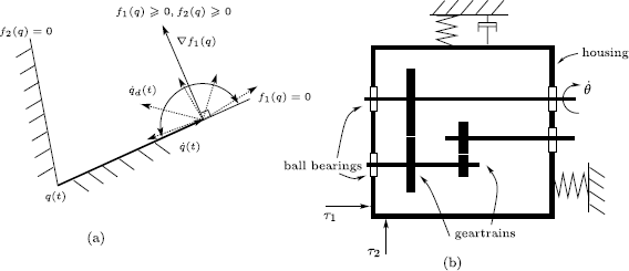
(a) The set of desired trajectories. (b) Gearbox system
-
3.
It is interesting to explore what happens when \(V(0)=0 \Leftrightarrow\ \dot{\tilde{q}}(0)=0\ \mbox{and}\ \tilde{q}(0)=0\). According to the above, \(V(t)=0\) for all \(t \geq 0\) if conditions (52) and (54) are satisfied. Since we have assumed that \(\dot{q}_{d}(\cdot)\) is continuous, so is \(\dot{q}(\cdot)\) and there is no impact. We therefore attain here the limitation of working with a motion controller and continuous desired velocities. However, if \(V(0)\neq 0\) then impacts may occur despite condition (52) and nothing guarantees from the above analysis that they vanish.
-
4.
Assume now that \(q_{d}(\cdot)\) is absolutely continuous, \(\dot{q}_{d}(\cdot)\) is right-continuous of local bounded variations with discontinuities at impact times \(t_{k}\). Then
$$\begin{aligned} \begin{aligned} \sigma_{V}(t_{k}) & =T_{L}(t_{k})+T_{L,d}(t_{k})+ \frac{1}{2}\biggl[\dot{q}_{d}\bigl(t_{k}^{+} \bigr)^{T}\tilde{M}(t_{k})\dot{q}_{d} \bigl(t_{k}^{+}\bigr)-\frac{1}{2}\dot{q}_{d} \bigl(t_{k}^{-}\bigr)^{T}\tilde{M}(t_{k}) \dot{q}_{d}\bigl(t_{k}^{-}\bigr)\biggr] \\ &\quad {} -\bigl[\dot{q}\bigl(t_{k}^{+}\bigr)M \bigl(q(t_{k})\bigr)\dot{q}_{d}\bigl(t_{k}^{+} \bigr)-\dot{q}\bigl(t_{k}^{-}\bigr)M\bigl(q(t_{k}) \bigr)\dot{q}_{d}\bigl(t_{k}^{-}\bigr)\bigr], \end{aligned} \end{aligned}$$(56)where \(\tilde{M}(t_{k})=M(q(t_{k}))-M(q_{d}(t_{k}))\), \(T_{L,d}(t_{k})=\frac{1}{2}\dot{q}_{d}(t_{k}^{+})^{T}M(q_{d}(t_{k})) \dot{q}_{d}(t_{k}^{+})- \frac{1}{2}\dot{q}_{d}(t_{k}^{-})^{T}M(q_{d}(t_{k}))\dot{q}_{d}(t_{k}^{-})\) is the desired kinetic energy loss, and \(T_{L}(t_{k})\) is the kinetic energy loss. If \(\dot{q}_{d}(\cdot)\) obeys the same impact law as \(\dot{q}(\cdot)\), then \(T_{L,d}(t_{k}) \leq 0\). Assume that \(\tilde{q}(0)=0\) and \(\dot{\tilde{q}}(0)=0\), \(f(q(0))> 0\). Then \(V(t)=0\ \Rightarrow\ \tilde{q}(t)=0\) and \(\dot{\tilde{q}}(t)=0\) for all \(t \in [0,t_{0})\). From (56) one has \(\sigma_{V}(t_{0})=0\) since both \(\dot{q}(\cdot)\) and \(\dot{q}_{d}(\cdot)\) jump at \(t_{0}\) with the same impact mapping. Let condition (54) hold, then \(V(\cdot)\) keeps vanishing during persistent contact. We infer that \(\tilde{q}(t)=0\) and \(\dot{\tilde{q}}(t)=0\) for all \(t \geq 0\). The next step is to analyse the closed-loop behaviour with initial tracking error. The idea is that if \(V(0)>0\) then the third and fourth terms between brackets in (56) may be upperbounded by a function \(\epsilon(V(0))\) of the initial error, with \(\epsilon(0)=0\). We conjecture that if impacts are separated enough (existence of a uniform large enough dwell-time, whose size depends on \(V(0)\)), then local stability may be shown, though the semi-negativeness of \(\dot{V}(\cdot)\) outside impacts is a weak property. For the sake of briefness, this is left as a future work. We nevertheless point out two cases in which impacts are separated: \(e_{\mathrm{n}}=0\) (plastic collisions) and \(e_{\mathrm{n}}=1\) (elastic collisions). In the first case, an impact is followed by a persistent contact phase. In the second case, it follows from [6, Proposition 4.11] that there exists a dwell-time separating impacts, which depends on the initial velocity.
-
5.
It is clear that the developments in Sects. 5 and 6 hold each time there is only one joint with clearance and all the other joints are actuated. The case of multiple clearances is more involved, though the numerical results in [4] indicate that PD, feedback linearization and passivity-based controllers possess remarkable robustness when applied to a four-bar system with one, two or three joint clearances. We may consider the system in Fig. 7(a), with joints \(J_{1}\), \(J_{2}\) and \(J_{3}\) actuated, and dynamics in (34). Mimicking Sect. 5, let us apply the same controller as (48) to subsystem \(S_{1}\) in (34)(a):
$$ \tau_{1}=M_{1}(q_{1})\ddot{q}_{1,d}+C_{1}(q_{1}, \dot{q}_{1})\dot{q}_{1,d}+G_{1}(q_{1})-K_{v} \dot{\tilde{q}}_{1}-K_{p}\tilde{q}_{1}. $$(57)We are led to analyse the stability with the Lyapunov candidate function (see (50) and (37)), that is, \(V(\tilde{q}_{1},\dot{\tilde{q}}_{1},q_{4},q_{5},\dot{q}_{4},\dot{q}_{5})=\frac{1}{2}\dot{\tilde{q}}_{1}^{T}M_{1}(q_{1})\dot{\tilde{q}}_{1}+\frac{1}{2}\tilde{q}_{1}^{T}K_{p}\tilde{q}_{1}+\frac{1}{2}\dot{q}_{4}^{T}M_{4}\dot{q}_{4}+U_{4}(q_{4})+\frac{1}{2}\dot{q}_{5}^{T}M_{5}\dot{q}_{5}+U_{5}(q_{5})\). After a few calculations we obtain \(\sigma_{V}(t_{k})=T_{L}(t_{k})-\dot{q}_{1,d}(t_{k})^{T}M_{1}(q_{1})\sigma_{\dot{q}_{1}}(t_{k})\) instead of (51), where \(T_{L}(t_{k})\) denotes the system’s kinetic energy loss. The variation of the term \(\dot{q}_{1,d}(t_{k})^{T}M_{1}(q_{1})\sigma_{\dot{q}_{1}}(t_{k})\) which by the impact dynamics equals \(\dot{q}_{1,d}(t_{k})^{T}{\mathcal{M}}_{14}(q_{1}(t_{k}),q_{4}(t_{k}))p_{\mathrm{n},u,14}(t_{k})\) is not easy to characterize through a simple condition as (52). During persistent contact phases, both controllers in (57) and (36) are equal, and doing the same calculations as in Sect. 5 we obtain along the closed-loop system’s trajectories: \(\dot{V}(t) \leq -\dot{\tilde{q}}_{1}^{T}K_{v}\dot{\tilde{q}}_{1}-\dot{q}_{1,d}(t)^{T}{\mathcal{M}}_{14}(q_{1},q_{4})\lambda_{\mathrm{n},14}(t)\). Again, the second term on the right-hand side is not guaranteed to be non-positive without further constraints on the desired trajectory. In case of regulation the desired velocity \(\dot{q}_{d}\) vanishes, and we can follow the same lines as in Sect. 5. Same ideas can be applied to the six-bar system in Fig. 6(a) with dynamics in (20)–(22), where one may choose to apply a torque \(\tau_{2}\) at joint \(J_{4}\), or not, and to the linkage in Fig. 3. In such cases it will be crucial to analyse the system’s performance as a function of how many and where actuators and sensors are mounted, and of clearances size. Indeed, these parameters will change the set of closed-loop fixed points, hence the precision of the system. Getting back to trajectory tracking, this preliminary analysis suggests that slow enough desired trajectories, or desired trajectories which switch between zero and non-zero (with a dwell-time allowing for \(V\) to be a non-monotonic Lyapunov function) should guarantee some kind of closed-loop stability property, even in the presence of multiple clearances.

7 Conclusions
Systems with joint clearance occupy a particular place within the set of controlled Lagrangian systems with unilateral constraints and impacts. Clearances are hard disturbances which augment the system’s dimension and add collisions and contact forces. Hence the major issues for the control of such systems, are the underactuation and the fact that the available output usually consists of partial positions and velocities, because measuring the whole state of the system with joint clearance is often technologically and economically impossible. There are two main control objectives, namely designing “simple” feedback controllers which possess some robustness w.r.t. mechanical play, or designing specific controllers which “compensate” for clearances and guarantee high accuracy. Most likely there does not exist a universal controller for systems with joint clearance because the choice of a control input depends on many parameters like system’s dimension, the number of joints with clearances, the size of the clearances, the contact parameters (restitution coefficients, friction), the precision and the number of sensors, the control objective—regulation, tracking, robustness, accuracy improvement, the degree of actuation, etc. In this paper we have reviewed and analysed three important families of feedback controllers: impactless with persistent contact, using impacts in a juggling systems framework, and PD + for regulation and tracking. Let us end with some open issues and comments (the list being obviously non-exhaustive):
-
1.
(State observers) Existing state observers [40, 56] measure the whole position vector \(q\) and estimate \(\dot{q}\), which does not really help in our case. As an example consider the mechanism in Fig. 4(b), actuated at \(J_{1}\) and with clearances at the other joints. Is it possible to design an observer which estimates part of the state of subsystem \(S_{2}=(\mathbf{B}_{2},\mathbf{B}_{3})\) (sensors may be mounted at some joints), from measurements of the state of subsystem \(S_{1}=(\mathbf{B}_{1})\)? Certainly contact phases and impacts have to be used (see [7, 40] for observability through the impacts).
-
2.
(Positive, switching, finite-time controls) Control with signed (non-negative) inputs stems from the unilaterality of the constraint and is present in Sects. 3 and 4. They may be signed impulsive inputs (in case of jugglers), or signed bounded inputs (in case of persistent contact). An interesting path is to investigate in which way the canonical dynamics in (26) could be used in the framework of persistent contact control of Sect. 3. Also the problem of stabilization using controllers which switch between several kinds of sub-controllers (persistent contact, with impacts, PD+), could enlarge the scope of applications of the above results, see Remark 4. Finite-time convergent schemes (like sliding-mode control [14, Sect. 7.5.5]) would be worth investigating as well. The time-discretization is also an important subject for contact tasks.
-
3.
(Accuracy) The set ℰ of equilibrium points that stems from the PD + gravity compensation input (Sect. 5), and consequently the accuracy of the closed-loop system, are influenced by the degree of actuation. Consider as an example the 6-bar system in Fig. 6(a): how does the addition/deletion of an actuator at joint \(J_{4}\) (the joints \(J_{1}\), \(J_{2}\) and \(J_{6}\) being actuated) modify the set of closed-loop equilibria? Studying the influence of the clearance-free system degree of actuation on the closed-loop accuracy (in addition to stability) is a crucial topic.
-
4.
(Vibrations active control) When the clearances are small enough, it is intuitively clear that the dynamical effects due to clearances could be assimilated to vibrations. Vibration analysis associated with ball bearings clearance may be found in [21, 32]. This could be used in a gearbox system as in Fig. 8(b) with clearances in the ball bearings and in the geartrains and imposed angular velocity \(\dot{\theta}\), with control inputs \(\tau_{1}\) and \(\tau_{2}\) designed to compensate for the vibration effects on the housing dynamics. However, this departs from the point of view adopted in this article and consequently this is not analysed.
Notes
In general, the dynamics could be written using Newton–Euler formalism. However, for control purposes the Lagrangian framework is the most suitable one; see, e.g. [18].
Hence, \(\dot{q}(t^{+})=\dot{q}(t)\) for all \(t \geq 0\).
Let us recall that the CoRs can be chosen non-constant, e.g. velocity dependent, to improve the model capabilities.
However, one does not necessarily have \(w_{c}(q(t),\dot{q}(t),\tau(t)) \leq 0\). All vector inequalities are understood as being componentwise.
More realistic gap functions would be with \(\alpha_{i}=\alpha_{i}(\theta_{2})\) depending on teeth geometry. We keep the simplest form in this short example.
From the Fundamental Principle of Dynamics, the CoM’s dynamics of a material system depends only on the external forces acting on the system.
It is, however, worth pointing out that even though existence conditions can be analysed, the explicit calculation of the zero dynamics may be hard.
References
Acary, V.: Projected event-capturing time-stepping schemes for nonsmooth mechanical systems with unilateral contact and Coulomb’s friction. Comput. Methods Appl. Mech. Eng. 256, 224–250 (2013)
Acary, V., Brogliato, B.: Numerical Methods for Nonsmooth Dynamical Systems. Applications in Mechanics and Electronics. Lecture Notes in Applied and Computational Mechanics, vol. 35. Springer, Berlin (2008)
Addi, K., Brogliato, B., Goeleven, D.: A qualitative mathematical analysis of a class of linear variational inequalities via semi-complementarity problems: applications in electronics. Math. Program. 126(1), 31–67 (2011)
Akhadkar, N., Acary, V., Brogliato, B.: Analysis of collocated feedback controllers for four-bar planar mechanisms with joint clearances. Multibody Syst. Dyn. 38(2), 101–136 (2016)
Ames, A.D., Galloway, K., Sreenath, K., Grizzle, J.W.: Rapidly exponentially stabilizing control Lyapunov functions and hybrid zero dynamics. IEEE Trans. Autom. Control 59(4), 876–891 (2014)
Ballard, P.: Formulation and well-posedness of the dynamics of rigid body systems with perfect unilateral constraints. Philos. Trans. R. Soc. Lond. A 359(1789), 2327–2346 (2001)
Baumann, M., Leine, R.I.: A synchronization-based state observer for impact oscillators using only collision time information. Int. J. Robust Nonlinear Control 26, 2542–2563 (2016)
Bernstein, D.S.: Matrix Mathematics. Theory, Facts, and Formulas with Application to Linear Systems Theory. Princeton University Press, Princeton (2005)
Blumentals, A., Brogliato, B., Bertails-Descoubes, F.: The contact problem in Lagrangian systems subject to bilateral and unilateral constraints,with or without sliding Coulomb’s friction: a tutorial. Multibody Syst. Dyn. 38, 43–76 (2016)
Bourgeot, J.M., Brogliato, B.: Tracking control of Lagrangian complementarity systems. Int. J. Bifurc. Chaos 15(6), 1839–1866 (2005)
Brogliato, B.: Absolute stability and the Lagrange–Dirichlet theorem with monotone multivalued mappings. Syst. Control Lett. 51(5), 343–353 (2004)
Brogliato, B.: Inertial couplings between unilateral and bilateral holonomic constraints in frictionless Lagrangian systems. Multibody Syst. Dyn. 29(3), 289–325 (2013)
Brogliato, B.: Kinetic quasi-velocities in unilaterally constrained Lagrangian mechanics with impacts and friction. Multibody Syst. Dyn. 32(2), 175–216 (2014)
Brogliato, B.: Nonsmooth Mechanics. Models, Dynamics and Control, third edn. Communications and Control Engineering. Springer, Berlin (2016)
Brogliato, B., Zavala-Rio, A.: On the control of complementary-slackness mechanical juggling systems. IEEE Trans. Autom. Control 45(2), 235–246 (2000)
Brogliato, B., Niculescu, S.I., Orhant, P.: On the control of finite-dimensional mechanical systems with unilateral constraints. IEEE Trans. Autom. Control 42(2), 200–215 (1997)
Brogliato, B., Mabrouk, M., Zavala-Rio, A.: On the controllability of linear juggling mechanical systems. Syst. Control Lett. 55, 350–367 (2006)
Brogliato, B., Lozano, R., Maschke, B., Egeland, O.: Dissipative Systems Analysis and Control. Theory and Applications, 2nd edn. Communications and Control Engineering. Springer, London (2007)
Byrnes, C.I., Isidori, A.: Asymptotic stabilization of minimum phase nonlinear systems. IEEE Trans. Autom. Control 36(10), 1122–1337 (1991)
Chang, S.L., Tsai, L.W.: On the redundant-drive backlash-free robotic mechanisms. ASME J. Mech. Des. 115, 247–254 (1993)
Changqing, B., Qingyu, X.: Dynamic model of ball bearings with internal clearance and waviness. J. Sound Vib. 294, 23–48 (2006)
Chevallereau, C., Westervelt, E.R., Grizzle, J.W.: Asymptotically stable running for a five-link, four-actuator, planar bipedal robot. Int. J. Robot. Res. 24(6), 431–464 (2005)
Duarte, F., Machado, J.T.: Describing function of two masses with backlash. Nonlinear Dyn. 56, 409–413 (2009)
Facchinei, F., Pang, J.S.: Finite-Dimensional Inequalities and Complementarity Problems, vol. I. Springer Series in Operations Research. Springer, Berlin (2003)
Flores, P., Ambrosio, J., Claro, J.P., Lankarani, H.: Kinematics and Dynamics of Multibody Systems with Imperfect Joints. Lecture Notes in Applied and Computational Mechanics, vol. 34. Springer, Berlin (2008)
Flores, P., Koshy, C., Lankarani, H., Ambrosio, J., Claro, J.: Numerical and experimental investigation on multibody systems with revolute joint clearance joints. Nonlinear Dyn. 65(4), 383–398 (2011)
Galeani, S., Menini, L., Potini, A., Tornambè, A.: Trajectory tracking for a particle in elliptical billiards. Int. J. Control 81(2), 189–213 (2008)
Glocker, C.: Set-Valued Force Laws. Lecture Notes in Applied Mechanics, vol. 1. Springer, Berlin (2001)
Glocker, C.: An introduction to impacts. In: Haslinger, J., Stavroulakis, G. (eds.) Nonsmooth Mechanics of Solids. CISM Courses and Lectures, vol. 485 pp. 45–102. Springer, New York (2006)
Guan, Y., Li, M., Lim, T., Jr, W.S.: Comparative analysis of actuator concepts for active gear pair vibration control. J. Sound Vib. 269, 273–294 (2004)
Hiriat-Urruty, J.B., Lemaréchal, C.: Fundamentals of Convex Analysis. Grundlehren text Editions. Springer, Berlin (2000)
Jang, G., Jeong, S.: Vibration analysis of a rotating system due to the effect of ball bearing waviness. J. Sound Vib. 269, 709–726 (2004)
Koshy, C., Flores, P., Lankarani, H.: Study of the effect of contact force model on the dynamic response of mechanical systems with dry clearance joints: computational and experimental approaches. Nonlinear Dyn. 73(1), 325–338 (2013)
Krinner, A., Thümmel, T.: Non-smooth behaviour of a linkage mechanism with revolute clearance joints. In: New Advances in Mechanisms, Transmissions and Applications. Proceedings of the Second Conference MeTrApp 2013. Mechanisms and Machine Science, vol. 17, pp. 233–241 (2014)
Lagerberg, A., Egardt, B.: Backlash estimation with application to automotive powertrains. IEEE Trans. Control Syst. Technol. 15(3), 483–493 (2007)
Lancaster, P., Tismenetsky, M.: The Theory of Matrices, 2nd edn. Academic Press, Orlando (1985)
Leine, R.I., van de Wouw, N.: Stability and Convergence of Mechanical Systems with Unilateral Constraints. Lecture Notes in Applied and Computational Mechanics, vol. 36. Springer, Berlin (2008)
Mata-Jimenez, M., Brogliato, B.: Analysis of PD and nonlinear control of mechanical systems with dynamic backlash. J. Vib. Control 9(1), 119–156 (2003)
McClamroch, N., Wang, D.: Feedback stabilization and tracking of constrained robots. IEEE Trans. Autom. Control 33(5), 419–426 (1988)
Menini, L., Tornambé, A.: Velocity observers for non-linear mechanical systems subject to non-smooth impacts. Automatica 38, 2169–2175 (2002)
Menini, L., Tornambè, A.: Control of (otherwise) uncontrollable linear mechanical systems through non-smooth impacts. Syst. Control Lett. 49(4), 311–322 (2003)
Menini, L., Possieri, C., Tornambé, A.: On the computation of the continuous-time reference trajectory for mechanical juggling systems. In: Proc. IEEE 54th Annual Conference on Decision and Control, Osaka, Japan, pp. 145–150 (2015)
Morarescu, C.I., Brogliato, B.: Trajectory tracking control of multiconstraint complementarity Lagrangian systems. IEEE Trans. Autom. Control 55(6), 1300–1313 (2010)
Moreau, J.J.: Unilateral contact and dry friction in finite freedom dynamics. In: Moreau, J.J., Panagiotopoulos, P. (eds.) Nonsmooth Mechanics and Applications. CISM Courses and Lectures, pp. 1–82. Springer, New York (1988)
Müller, A.: Internal preload control of redundantly actuated parallel manipulators–its application to backlash avoiding control. IEEE Trans. Robot. 21(4), 668–677 (2005)
Nguyen, N., Brogliato, B.: Multiple Impacts in Dissipative Granular Chains. Lecture Notes in Applied and Computational Mechanics, vol. 72. Springer, Berlin (2014)
Nordin, M., Gutman, P.: Controlling mechanical systems with backlash—a survey. Automatica 38, 1633–1649 (2002)
Nordin, M., Galic, J., Gutman, P.: New models for backlash and gear play. Int. J. Adapt. Control Signal Process. 11, 49–63 (1997)
Paden, B., Panja, R.: Globally asymptotically stable ‘PD+’ controller for robot manipulators. Int. J. Control 47(6), 1697–1712 (1988)
Paoli, L., Schatzman, M.: Penalty approximation for dynamical systems submitted to multiple non-smooth constraints. Multibody Syst. Dyn. 8(3), 347–366 (2002)
Pereira, C., Ramalho, A., Ambrosio, J.: A critical overview of internal and external cylinder contact force models. Nonlinear Dyn. 63(4), 681–697 (2011)
Pfeiffer, F., Glocker, C.: Multibody Dynamics with Unilateral Contacts. Nonlinear Science. Wiley, New York (1996)
Reyhanoglu, M., van der Schaft, A., McClamroch, N., Kolmanovsky, I.: Dynamics and control of a class of underactuated mechanical systems. IEEE Trans. Autom. Control 44(9), 1663–1671 (1999)
Saperstone, S., Yorke, J.: Controllability of linear oscillatory systems using positive controls. SIAM J. Control 9(2), 253–262 (1971)
Spong, M.W., Kelly, R., Ortega, R.: Comments on “Adaptive manipulator control: a case study”. IEEE Trans. Autom. Control 35(6), 761–762 (1990)
Tanwani, A., Brogliato, B., Prieur, C.: Observer design for unilaterally constrained Lagrangian systems: a passivity-based approach. IEEE Trans. Autom. Control 61(9), 2386–2401 (2016)
Thuemmel, T., Rossner, M.: Introduction to modelling and parameter identification methodology of linkages by measurements and simulation. In: Proceedings of 13rd World Congress in Mechanisms and Machine Science, Guanajuato, Mexico, 19–25 June, pp. IMD-123 (2011)
Thümmel, T., Ginzinger, L.: Measurements and simulations of a crank and rocker mechanism including friction, clearance and impacts. In: Proceedings of IXth Intern. Conf. on the Theory of Machines and Mechanisms, August 31–September 02, Liberec, Czech Republic (2004)
van de Wouw, N., Leine, R.I.: Attractivity of equilibrium sets of systems with dry friction. Nonlinear Dyn. 35(1), 19–39 (2008)
Varedi, S., Daniali, H., Dardel, M., Fathi, A.: Optimal dynamic design of a planar slider–crank mechanism with a joint clearance. Mech. Mach. Theory 86, 191–200 (2015)
Xiao, H., Shao, Y., Brennan, M.: On the contact stiffness and nonlinear vibration of an elastic body with a rough surface in contact with a rigid surface. Eur. J. Mech. A, Solids 49, 315–328 (2015)
Yan, S., Xiang, W., Zhang, L.: A comprehensive model for 3D revolute joints with clearances in mechanical systems. Nonlinear Dyn. 80(1), 309–328 (2015)
Zavala-Rio, A., Brogliato, B.: On the control of a one degree-of-freedom juggling robot. Dyn. Control 9, 67–90 (1999)
Zavala-Rio, A., Brogliato, B.: Direct adaptive control design for one-degree-of-freedom complementary-slackness jugglers. Automatica 37, 1117–1123 (2001)
Author information
Authors and Affiliations
Corresponding author
Rights and permissions
About this article

Cite this article
Brogliato, B. Feedback control of multibody systems with joint clearance and dynamic backlash: a tutorial. Multibody Syst Dyn 42, 283–315 (2018). https://doi.org/10.1007/s11044-017-9585-4
Received:
Accepted:
Published:
Issue Date:
DOI: https://doi.org/10.1007/s11044-017-9585-4