Home automation - an IoT based system to open security gates using number plate recognition and artificial neural networks

Abstract

This paper proposed a system that automatically opens security gates. A system is designed and implemented to automatically open security gates for vehicles using Licence Plate Recognition. Image processing is used to extract the licence plate and characters, and an Artificial Neural Network is used to perform Optical Character Recognition on licence plate characters. Internet of Things principles are introduced to the system to allow for web and mobile application integration. A proximity sensor is designed to detect vehicles and to start the recognition process. An ambient light sensor and control circuit is developed to control ambient lighting conditions using an ambient light source. The neural network achieved an accuracy of 88% on training data and 93% on licence plate characters. A unique strong point of the system is the ability to monitor and control the system using a web interface or mobile application. The system is also able to produce mobile notifications regarding security gate access attempts.

1 Introduction

Access control at security gates is typically implemented in a manner that requires user input. Traditional implementations for vehicle access require the use of a pressure plate, remote control, keypad or a Radio Frequency Identification (RFID) tag, which could cause inconvenience for a user or have security concerns. It is desired for the access control process to be automated to save time and increase convenience. Home automation has become more popular over the years since it allows devices to work together to automatically complete tasks with the goal of simplifying daily routines [17]. Another emerging technology is known as the Internet of Things (IoT) which is best described as connecting ordinary objects, appliances, sensors or actuators to the Internet to perform tasks which could support the home automation process [25]. To overcome the limitations of traditional access control systems, the system should be incorporated into a home automation system using IoT techniques.

To improve on the limitations of traditional access control for vehicles, a method to improve on convenience as well as security should be considered. Recently the use of cameras to validate access for vehicles is increasing. Images are used to identify vehicles and Optical Character Recognition (OCR) extract licence plate data to perform access control [16]. The method of detecting and extracting character data from a licence plate using image acquisition and OCR is also known as Licence Plate Recognition (LPR) [12]. Using LPR for access control eliminates user interaction and promotes automation. Limiting factors of traditional access control methods includes that pressure plates do not provide security but only detection, RFID tags could be stolen and are inconvenient to use in rainy weather and a remote control has the disadvantage of being battery operated or the signal could be reproduced [12]. When considering these limitations, it becomes apparent that a LPR system is ideal to use for automated access control by integrating it via IoT principles into a home automation system.

The LPR process relies on a system of image acquisition to find and recognise licence plate characters. When examining a LPR system from a high level of design abstraction it consists of the following two characteristics: detecting the region of interest (ROI) of the licence plate in an image, and the detection of licence plate characters within the ROI [4, 12]. A more in depth description is a system that follows the following order of operation: (1) image acquisition; (2) number plate extraction; (3) character segmentation and (4) character recognition [20].

This paper discusses the design and implementation of a system to automatically open security gates using LPR and an Artificial neural networks (ANN) for OCR. The hardware of the system is designed from first principles. For image processing, a combination of open source and first principle software is used. The ANN is designed from first principles in the C++ language. A web-interface and mobile application is developed as part of incorporating IoT principles. The findings and results of the accuracy and validity of the design is also discussed.

This paper applied sensors, wireless P2P communication, and 3G technologies to present the design and development of a home automation for number plate recognition.

The scientific contribution of the proposed system lies in the design and development of Artificial Neural Network and partially image processing algorithms from first principles to be used for character identification within the license plate recognition system. However, none of the existing related works which are detailed in the next section have addressed the details of implementation from first principles with high accuracy but mainly libraries and off the shelf components were used.

This paper is organised as follows. Section 2 describes some related work to successfully complete this project. Section 3 provides an overview of the system that was developed. Within Section 4, the design and implementation of the system can be found, where a solution was implemented with regards to functionality and cost effectiveness. The results and findings throughout the design and implementation phase is summarised in Section 5. Some proposed future work and research regarding the design is discussed in Section 6, with the conclusion in Section 7.

2 Related works

Various solutions of extracting a ROI of a licence plate exist, but the process could be difficult due to different background objects, colours and conditions. A solution proposed in [4] states that the features of a licence plate is known such as shape, height and width. This can be used to ease the detection of the ROI. This solution also incorporates edge detection as the shape of a licence plate is rectangular. It should be noted that the solution in this is not robust since only edges of a certain colour are detected which could lead to weak performance in dark situations. Another solution is proposed by [15], where canny edge detection forms the basis of the licence plate detection. This method works by first resizing an image which is then converted to greyscale. A binary threshold operation occurs next to aid the edge detection algorithm. Filtering is applied to the image and an edge detection algorithm detects edges within the modified image. The detected edges can be used to determine the ROI. A method proposed in [12], follows the following order of operation to determine the ROI of an image containing a licence plate: (1) convert the image to greyscale; (2) perform a threshold operation (convert to a binary image); (3) perform filtering whilst preserving edges; and (4) Sobel edge detection to reduce noise whilst detecting edges. Overall it can be seen that the detection of a licence plate within an image is somewhat trivial, and in all cases, is solved on a high-level design as follows: (1) input an image; (2) pre-processing; (3) image filtering (4) edge detection or more specifically rectangle detection and finally (5) extraction. These steps are also illustrated in a method proposed by [14].

Using the ROI, an image containing a licence plate can be produced. To detect individual characters, a segmentation algorithm should be applied to this image. The purpose of a segmentation algorithm is to separate the characters contained within the image of a licence plate into separate objects [19]. The separate characters are then recognised by a recognition algorithm. Horizontal and vertical projection and extracting characters from horizontal segments is the method described by [18] to extract characters from the licence plate ROI. To implement this, histogram-based segmentation could be implemented to promote simplicity and ease of implementation [19]. An algorithm iterates for the number of horizontal pixels in the ROI of the licence plate. Each vertical pixel is counted to produce a histogram containing the number of vertical pixels at each horizontal position. The histogram is stored in a data container. By iterating through the histogram in the data container, the start and stop pixel positions for characters can be determined, allowing segmentation to take place. Each character is saved as a separate image for use in the recognition algorithm. This is also known as vertical projection.

Character recognition can be divided into two main categories. The categories consist of online and offline methods. Online character recognition involves the recognition of characters written in real time such as character recognition on a smartphone or writing tablet. This method is not intended for LPR which consist of a fully complete image to recognise. Offline character recognition however recognises a predefined image such as a scanned document or image which is ideal for the LPR process. Furthermore, offline character recognition can consist of methods, such as clustering, feature extraction, pattern matching or ANN’s [5]. According to [24], another method for OCR in the case of LPR is the hidden Markov model. The use of an ANN should prove advantageous in the LPR situation since ANN’s are proven tools in finding pattern solutions and require less formal statistical training than other methods for OCR [23].

A possible solution of integrating an LPR system is to detect the presence of an approaching vehicle, then checking the authentication of the vehicle on a local database and opening a garage door if the vehicle has access permission [1]. The approach of this system is ideal with the limitation of local database integration. For an integrated home automation LPR system, Internet connectivity is a requirement. Various design techniques exist for the five steps of the LPR processes above which will be described in more detail. The novelties within this paper includes: Integration of ANN with web-hosted storage to eliminate local database integration as a failsafe, the ability to integrate with existing gate motors on the market, improving on traditional access control for personal use whilst promoting cost effectiveness and integrating IoT principles, and finally the design of a cost-effective proximity sensor to detect the presence of a vehicle.

3 System overview

The proposed approach is to, (1) detect the presence of a vehicle using a proximity sensor; (2) adjust the ambient light if necessary using an ambient light sensor and ambient light source; (3) acquire an image of the front of a vehicle with a USB based camera; (4) extract the licence plate; (5) extract the characters; (6) recognise and validate characters using an ANN; (7) open the security gate using the gate interface; (8) integrate IoT principles into the project. A high-level system overview can be seen in Fig. 1. For the main processor, an Odroid C2 computer is used. It is a mobile, powerful and cost effective solution that provides various interface technologies for future system expansion. The system is connected to the Internet using a 3G dongle. The Odroid communicates wirelessly to the gate interface via wireless transceiver modules in order to send commands capable of opening an existing security gate. An overview of the software design for the system can be seen in Fig. 2.

Fig. 1

System hardware overview

Fig. 2

System software overview

4 System design

4.1 Proximity sensor

For the system to start, it should be able to detect if a vehicle is present. This is important to save system resources. We designed and implement a proximity sensor using an IR based distance sensor which provides an analogue voltage as output that is proportional to the distance measured. The sensor is powered using 4.5–5.5 V Direct Current (DC). When the output voltage to distance curve of the sensor is studied, it is found that the output voltage of the sensor (v _{d i s t} ) lies within the rage, 0.5 V ≤ v _{d i s t} ≤ 2.6 V DC with minor fluctuations with different colour objects. When examining the output voltage of the sensor and taking into consideration the specifications of the ADC of the Odroid (maximum ADC voltage 1.8 V), it is clear that some circuit conditioning is necessary in order to safely interface the proximity sensor with the Odroid at a maximum signal voltage of 1.8 V. An ideal solution is to condition the distance meter output to a digital signal, meaning the signal should be off at 0 V, or on at 1.8 V. As presented in [21], a voltage comparator is used. Background theory of voltage comparators states the following. Given the inverting input (v _n ), non-inverting input (v _p ) and output voltage (v _o ) of an operational amplifier, v _o will latch to a high state (on) if v _p > v _n , otherwise v _o will latch to a low state (off). The output voltage curve of the distance sensor was measured to determine the threshold voltage to set for v _n , since the sensor voltage, v _{d i s t} is connected to v _p of the operational amplifier. The following measurements in Table 1 are obtained using a digital multimeter.

Table 1 Distance to voltage relationship of distance sensor

As Table 1 indicates, the voltage the sensor produces decreases as the distance increases, thus we used this property to detect proximity - knowing with the voltage being high, an object is in proximity. We power the circuit using 12 V, regulated down to 5 V using a 5 V fixed-voltage regulator (LM7805 series). To set a trigger voltage, the values in Table 1 is studied. Since the sensor detects distances less than 150 cm, we chose to set the threshold voltage at 200 mV. The threshold voltage is produced using a simple voltage divider, tapped from the regulated 5 V. This can be seen in (1), where R2 is chosen as 1 kΩ, and R1 is calculated as 24 kΩ. To safely interface the digital voltage with the Odroid, a variable-voltage regulator (LM317 series) is used. To set a maximum voltage of 1.8 V, (1) is used to set the resistance values for the regulator.

$$\begin{array}{@{}rcl@{}} \begin{array}{llllllll} V_{desired} &= V_{in}\left( \frac{R2}{R2+R1} \right)\\ 0.2 &= 5 \left( \frac{1000}{1000+R1} \right) \\ R1 &= 24\ k{\Omega} \end{array} \end{array} $$

(1)

In the case of the regulator calculation in (2), R1 _{r e g} is chosen as 680 Ω, and R2 _{r e g} is calculated as 300 Ω (which is used as a guideline to come close to 1.8 V).

$$\begin{array}{@{}rcl@{}} \begin{array}{llllllll} V_{odroid} &= 1.25 \left( 1+\frac{R2_{reg}}{R1_{reg}} \right)\\ 1.8 &= 1.25 \left( 1+\frac{R2_{reg}}{680} \right)\\ R2_{reg} &= 300\ {\Omega} \end{array} \end{array} $$

(2)

Initial prototyping testing on veroboard yielded inconsistent distance triggering results and after debugging it was found that due to a long 12 V power line, noise was present on the power rail. This was fixed by adding a capacitor at the 12 V power input to the circuit. The value for this capacitor is empirically determined as C _{n o i s e} = 100 n F. The final circuit diagram can be seen in Fig. 3, and a printed circuit board (PCB) layout is also designed and manufactured for this design.

Fig. 3

Proximity sensor schematic

The proximity sensor software is hosted on the Odroid. The Odroid periodically checks the input from the proximity sensor, and if a vehicle is detected, a flag is set on the Odroid to indicate the presence of a vehicle. If the flag was set, the next stage of software execution in the main system is started - that is image acquisition. In Fig. 4, the software flow of the proximity sensor can be seen. In the sample phase, an average of 50 samples are taken to filter out any present noise.

Fig. 4

Proximity sensor software flow

The final developed PCB of the proximity sensor can be seen in Fig. 5, with the sensor enclosure in Fig. 6.

Fig. 5

Proximity sensor populated PCB

Fig. 6

Proximity sensor and enclosure

4.2 Ambient light sensor and control circuitry

After the proximity of a vehicle is detected, a photo needs to be captured of the vehicle to acquire an image of its licence plate. For the system to be able to capture images in a range of ambient lighting conditions, an ambient light sensor and ambient light control circuit are designed, which consists of hardware and software components explained below.

After the proximity sensor is implemented, one ADC remained unused on the Odroid, thus the ambient light sensor can be implemented using an LDR. It is chosen to make use a reference voltage produced by the Odroid’s General-purpose input/output (GPIO) pins. The GPIO voltage is V _{g p i o} = 3.3 V. Since the ADC of the Odroid supports of a maximum voltage of 1.8 V, a resistor divider is constructed to produce a reference voltage, V _{r e f} = 1.8 V from V _{g p i o} . This can be seen in (3), where R2 is chosen as R2 = 1 kΩ and R1 is calculated as R1 = 833 Ω.

$$\begin{array}{@{}rcl@{}} \begin{array}{llllllll} V_{ref} &= V_{gpio} \left( \frac{R2}{R1+R2} \right) \\ 1.8 &= 3.3 \left( \frac{1000}{R1 + 1000} \right)\\ R1 &= 833\ {\Omega} \end{array} \end{array} $$

(3)

The LDR configuration can be seen in Fig. 7, the final circuit diagram for the ambient light sensor and ambient light control circuitry. The LDR is used in a resistor divider configuration with a resistor (R _g = 100 kΩ) to ground. Since the properties of an LDR produces a very large resistance in dark environments, and a low resistance in light environments, the LDR output voltage (V _{l d r} ) will change using resistor divider properties and the ADC of the Odroid measures V _{l d r} to determine the ambient lighting conditions. Measurements taken using a digital multimeter indicates that at very bright conditions, an LDR resistance of R _{l d r} ≤ 200 Ω is produced, and in dark conditions, R _{l d r} ≥ 2 MΩ. To see the effects of the ambient light conditions on V _{l d r} , (4) is used.

$$\begin{array}{@{}rcl@{}} \begin{array}{llllllll} V_{ldr} &= V_{ref} \left( \frac{R_{g}}{R_{ldr}+R_{g}} \right)\\ V_{ldr} &= 1.8 \left( \frac{100000}{R_{ldr}+ 100000} \right) \end{array} \end{array} $$

(4)

Fig. 7

Ambient light sensor and control circuitry schematic

Considering (4), it can be seen that if it is very dark, the voltage V _{l d r} that the ADC measures is low, and if it is light, the voltage is high. Since it is possible to measure the ambient light, a method is developed to turn the ambient light source on and off. We used a relay (PCH-112D2H), with a 12 V D C coil with a series resistance of R _{c o i l} = 260 Ω. A method to switch high voltage and high current applications using a small voltage is with the use of a BC337-40 NPN transistor. In Table 2, important characteristics of the transistor can be seen.

Table 2 Transistor properties

The maximum current rating of the relay is enough to drive the ambient light source (LED). The current required by the relay coil is measured to be 46 m A. This is also known as the collector current (I _c ). Given the value of I _c , the information in Table 2, and the voltage of an Odroid pin V _{o d r o i d} = 3.3V, a value for a base resistor (R _b ) is calculated to control the amount of current flowing through the base of the transistor (I _b ). This is shown in (5) and (6).

$$\begin{array}{@{}rcl@{}} \begin{array}{llllllll} I_{c} &= \beta \times I_{b}\\ 46\times10^{-3} &= 250 \times I_{b} \\ I_{b} &= 184\ \mu A \end{array} \end{array} $$

(5)

$$\begin{array}{@{}rcl@{}} \begin{array}{llllllll} R_{b} &= \frac{V_{odroid} - V_{be}}{I_{b}}\\ R_{b} &= \frac{3.3-1.2}{184\times 10^{-6}}\\ R_{b} &= 11.41\ k{\Omega} \end{array} \end{array} $$

(6)

Connecting a relay to a microcontroller or board such as the Odroid requires some protection circuitry. As stated in [7], changing current in a coil creates a voltage, thus if current in a coil changes rapidly, a high voltage is induced. Since a relay changes on and off states very rapidly, it is important to include protection circuitry known as a transient suppression network to protect sensitive electronics (in this case the Odroid). A simple protection diode (D1) is used in parallel over the relay coil. The diode minimises the induced voltage that could harm the Odroid.

The final design, including all values calculated in this section is shown in Fig. 7. Software to measure the ambient light and enable the relay to power the ambient light source was developed. The flow of the software can be seen in Fig. 8. In the sampling stage, averaging was applied to ensure that noise was filtered out. In Fig. 9, the populated PCB can be seen, and in Fig. 10, the enclosure can be seen.

Fig. 8

Ambient light sensor and control circuitry software flow

Fig. 9

Ambient light sensor and control circuitry populated PCB

Fig. 10

Ambient light sensor and control circuitry enclosure

4.3 Ambient light source

The ambient light source is used to improve ambient lighting conditions if it is too dark. LED’s are chosen as the light source due to low power consumption and minimal heat build-up. A set of 3 × 3 LED strips is used. The LED’s are powered by the ambient light sensor and control circuitry at 12 V. An enclosure with a two-pin socket and plug is constructed to house the light source. The ambient light source did not need a software component since it is controlled by the hardware and software of the ambient light sensor and control circuitry after an ambient light test is conducted. If the light source is activated, it is deactivated directly after the image acquisition phase of the system. In Fig. 11, the ambient light source that is implemented can be seen.

Fig. 11

Ambient light source

4.4 Camera

The camera that is chosen for the system had to satisfy some specifications such as cost and ease of installation, whilst also producing quality images with a satisfactory resolution to be able to identify licence plate characters at a distance of at least 2 meters from the camera. The Odroid USB-CAM 720P is used, a USB web-cam with a resolution of 1280 × 720. Refer to Fig. 12. With this camera, images are readable at 2-4 m in the day.

Fig. 12

Camera for the system

4.5 Image processing

The image processing software is used to convert the image taken in the acquisition phase to a format that could be used by the ANN to detect characters. A mixture of open-source helper functions and first principle software design is used to complete this part of the system. The image processing included the following categories.

• Image pre-processing.

• Licence plate segmentation.

• Licence plate character segmentation.

• Image conversion to ANN readable format.

With the start of the image processing, the original captured image are read into a matrix O. The size of the matrix is defined as [x × y], where x is the horizontal resolution of the image, and y the vertical resolution. Each element of the matrix (p _{y x} ), represents a pixel of the image, where every value p _{y x} is a vector of size [1 × 3], containing colour information of the pixel. Thus, colour information in each value of p _{y x} could take on three values known as blue, green and red (BGR). Each BGR value could be in the range such that p _b ,p _g ,p _r ∈ [0,225]. An example of the matrix can be seen in (7) with, x = 1280 and y = 720. An example of a pixel value can be seen in (8).

$$\begin{array}{@{}rcl@{}} \mathbf{O} &=& \left[\begin{array}{llllllll} \mathbf{p_{11}} & \mathbf{p_{12}} & {\dots} & \mathbf{p_{1x}}\\ \mathbf{p_{21}} & \mathbf{p_{22}} & {\dots} & \mathbf{p_{2x}}\\ {\vdots} & {\vdots} & {\ddots} & \vdots\\ \mathbf{p_{y1}} & \mathbf{p_{y2}} & {\dots} & \mathbf{p_{yx}} \end{array}\right] \end{array} $$

(7)

$$\begin{array}{@{}rcl@{}} \mathbf{p_{yx}} &=& \left[\begin{array}{llllllll} p_{b} & p_{g} & p_{r} \end{array}\right] \end{array} $$

(8)

At this stage of the image pre-processing, colour information is of no value, thus a greyscale operation is applied to the image. The greyscale image is the same size as O, but the pixel vector is changed to a size [1 × 1], where each pixel only consists of a single value, p ∈ [0,255]. Thus p = g r e y s c a l e(p _{y x} ), where p is the value of the grayscale pixel. Two methods are used for the greyscale operation, the first one is the greyscale function of OpenCV. The algorithm converts the original image (O) to a greyscale image (O _g ). The parameter CV_BGR2GRAY, is a global constant indicating the BGR colour to greyscale operation.

The second method for greyscale is the design of a greyscale function. According to the International Telecommunications Union (ITU), various implementations of greyscale exist. The ITU-R BT.709-6 [10] method is implemented. An algorithm is developed to convert the colour image O to greyscale O _g , using the coefficients proposed in ITU-R BT.709-6, where each grey pixel (p) is calculated by

$$\begin{array}{@{}rcl@{}} p = (0.0722\times B) + (0.7152\times G) + (0.2126\times R) \end{array} $$

(9)

The greyscale image of the licence plate, O _g , is given to an edge detector algorithm. Edge detection is a process in image processing that is used to detect boundary changes in images. Edge detection works by detecting sudden changes in reflectance, brightness or depth, and is used in various computer vision applications [2]. According to [3], the steps to completing Canny edge detection involves:

• 1. Smoothing the image and filtering out noise using a Gaussian filter.

• 2. Calculate edge strength or absolute size of the edge (G) and angle (𝜃), thus giving an intensity gradient G ∠ 𝜃.

• 3. Applying non-maximum suppression (thinning of the edge line).

• 4. Applying hysteresis.

After performing edge detection on O _g , the edge detection result is saved as O _e .

The method that we chose to detect a licence plate is known as contour detection. A contour can be defined as an outline that represents, or bounds a shape. Since edge detection is applied to O _g , the greyscale image, and produces the result O _e , finding a contour that represents the outline of a licence plate is easier than using only O, the original image. An OpenCV function (findcontours) to detect contours is used. A vector is produced containing all the contours in the image (O _e ). It is saved as output. Given the vector (output) containing the detected contours, an algorithm that validates each contour to a set of rules are developed. The rules are set to define a valid licence plate, and includes the following regarding a plate: width, height, area and aspect ratio. The following rules were applied to get a valid licence plate.

• 1. The plate candidate width needs to be greater than its height.

• 2. The plate candidate area needs to be satisfactory.

• 3. The plate candidate aspect ratio needs to be satisfactory.

• 4. Finally, a function counts internal contours of the plate candidate, and if it is satisfactory, the plate is saved into a matrix (O _p ).

The image processing upto this stage can be seen in Fig. 13, where the licence plate extraction is illustrated.

Fig. 13

Licence plate extraction example

To start character detection, the image of the licence plate is processed to improve the readability of the licence plate characters. Thresholding (binarization) is applied on the greyscale of the licence plate, O _p . An algorithm is designed to iterate through each horizontal and vertical pixel of O _p . Since a greyscale image is made out of pixels with a 1 × 1 vector in the range p ∈ [0,255], a cut-off value is chosen as T h r e s h o l d = 200, thus any pixel with a value lower is turned off, and any pixel with a value higher is turned on, saving the result in O _b . An example can be seen in Fig. 14.

Fig. 14

Binarization of licence plate

Two methods are implemented to extract a character, the first is the design of a character extraction platform using horizontal and vertical projection. The vertical projection can be seen in Fig. 15 and is used to cut out the letters. In Fig. 16, the horizontal projection for the character “C” can be seen, and is used to remove remaining white space. Vertical projection counts vertical pixels at each horizontal position to determine character positions from histogram peaks. Each detected peak is then also processed by the horizontal projection algorithm to produce the final result of a vector full of characters (O _c ). O _c is defined in (10), where c _n is an image of an extracted character, and n is the number of characters in the licence plate.

$$\begin{array}{@{}rcl@{}} \mathbf{O_{c}} &=& \left[\begin{array}{llllllll} \mathbf{c_{1}}&\mathbf{c_{2}}& {\dots} & \mathbf{c_{n}} \end{array}\right] \end{array} $$

(10)

Fig. 15

Vertical projection example

Fig. 16

Horizontal projection example

In addition to this an alteration of the contour detection algorithm is also applied to the licence plate to find contours (possible characters). Valid characters are defined by the following rules (South African licence plates).

• 1. Character width needs to be less than letter height.

• 2. Character area in range, a r e a ∈ [1700,4000]

• 3. Given that valid licence plate Character should have the dimensions 35 m m × 75 m m, the aspect ratio rule is chosen to be in a range, a s p e c t r a t i o ∈ [1.2,3].

Regardless of the method, the character detection and extraction procedure can be seen in Fig. 17. Finalising the character extraction algorithm, each extracted character was resized to a normalised size of 8 × 8 pixels, and binary inverted.

Fig. 17

Character extraction and normalisation

In Fig. 18, the extracted “C” of the licence plate can be seen. Due to the resize operation, the image is blurred, meaning it is now a greyscale image again. An image to text algorithm is designed to write scaled pixel values to a comma separated text file using (11). A scaled value of s c a l e d = 0, represents a black pixel, 0 < s c a l e d < 1 represents a grey pixel, whilst s c a l e d = 1 represents a white pixel. The algorithm converts all n characters in O _c to the text file, where each c _n is represented on a new line, and each line contained the scaled pixel values of a c _n .

$$\begin{array}{@{}rcl@{}} scaled &= \frac{pixel\ value}{255} \end{array} $$

(11)

Fig. 18

Extracted character “C”

An example for the line calculated for the character “C” in Fig. 18 can be seen in (12), where the line is displayed in matrix form using a modulo operation of 8. Each c _n is thus represented as a matrix of 8 × 8, or as a line of 64 numbers that are comma separated in a text file for example: 0,0.6,1,1,1,1,1,0,0,1,1,0,0……,0.

$$\begin{array}{@{}rcl@{}} \mathbf{line} &=& \left[\begin{array}{llllllll} 0 & 0.6 & 1 & 1 & 1 & 1 & 1 & 0 \\ 0 & 1 & 1 & 0 & 0 & 1 & 1 & 0 \\ 0.9 & 1 & 0.6 & 0 & 0 & 1 & 1 & 0 \\ 0.9 & 1 & 0.6 & 0 & 0 & 0 & 0 & 0 \\ 1 & 1 & 0.6 & 0 & 0 & 0 & 0 & 0 \\ 1 & 1 & 0.6 & 0 & 0 & 0 & 1 & 0.9 \\ 0.9 & 1 & 1 & 0 & 0 & 1 & 1 & 0 \\ 0 & 0 & 1 & 1 & 1 & 1 & 0 & 0 \end{array}\right] \end{array} $$

(12)

4.6 Character recognition using an artificial neural network

It should be noted that the term ANN and neural network refers to the same concept. Conventional computers are extremely fast and efficient in completing tasks and instructions that were programmed for them. The human brain, although operating magnitudes slower than a computer, are in cases far better in solving complex visual problems [34]. This phenomenon has driven the advancement and development of better ANN’s over the years, and is why an ANN is chosen to solve the visual problem of OCR on licence plate characters.

According to [34], a neural network can be defined as a physical cellular system which can acquire, store, and utilize experimental knowledge. ANN’s can thus complement existing computers to solve complex patterns, as well as learn by experience. An ANN is built upon the idea that we can to an extent build an artificial network with some of the power of the biological brain. In theory, this is possible by constructing an interconnected mesh of nodes called neurons. The mesh is organised into various layers, interconnecting the neurons using weights. The weights can be modified in a process called learning, to improve the accuracy of the network. The architecture of the ANN will be discussed later. An example of a neuron is shown in Fig. 19.

Fig. 19

Architecture of a neuron

A neuron consists of a number of inputs (x ₁…x _n ), weights (w ₁…w _n ), a summing junction (Σ), a bias (b), an activation function (f), and an output (y). The output of the summing junction can be seen in (13), and the output of a single neuron can be seen in (14).

$$\begin{array}{@{}rcl@{}} sum = {\sum}_{k = 1}^{n} \left( w_{k}\times x_{k}\right)+ b \end{array} $$

(13)

$$\begin{array}{@{}rcl@{}} y = f \left( sum \right) \end{array} $$

(14)

The activation function (f) is used to limit the output of the summing junction in a range that is determined by the chosen function. Various activation functions exist, but the log-sigmoid function is chosen. Using the log-sigmoid function, s u m ∈I R, and f(s u m) ∈ (− 1,1). The log-sigmoid function can be seen in (15).

$$\begin{array}{@{}rcl@{}} f \left( x \right) = \frac{1}{1+e^{-x}} \end{array} $$

(15)

All the neurons should be initialised by assigning values to their weights and biases. To assign values to weights and biases, the use of a uniform random number generator with mean (μ = 0) and standard deviation (σ = 1) is used, and scaled using (16). The initialisation of the initial weights and biases are a crucial part of the ANN initialisation [34].

$$\begin{array}{@{}rcl@{}} random = random \times \frac{1}{\sqrt{n}} \end{array} $$

(16)

Given the architecture of a neuron, a mesh can be constructed. This mesh is known as an ANN, and can be seen in Fig. 20. Each of the nodes in the ANN architecture are neurons, with all the components in Fig. 19. The inputs (X), number of hidden neurons, number of hidden layers, and outputs (Y) of the neural network can be scaled to any number. In the input layer, there can be 1 to j inputs. There can be any number from 1 to n hidden layers, each with a different number of hidden neurons such as i or k. The output layer can also consist of any number such as 1 to m outputs.

Fig. 20

Architecture of a neural network

As seen in Fig. 20, each neuron is connected to all neurons in the next layer. The connections are known as weights. Given an input vector X to the network, each neuron performs the calculation in (14). The calculations propagates through the network in a process called forward propagation to produce the output vector Y, where X is defined in (17) and Y in (18). Generalised formulas for the outputs of the neurons in the network can be seen in (19), (20), (21) and (22).

$$\begin{array}{@{}rcl@{}} \mathbf{X} &=& \left[\begin{array}{llllllll} x_{1}\\ x_{2}\\ \vdots\\ x_{j} \end{array}\right] \end{array} $$

(17)

$$\begin{array}{@{}rcl@{}} \mathbf{Y} &=& \left[\begin{array}{llllllll} y_{1}\\ y_{2}\\ \vdots\\ y_{j} \end{array}\right] \end{array} $$

(18)

$$\begin{array}{@{}rcl@{}} y_{j} = x_{j} \end{array} $$

(19)

$$\begin{array}{@{}rcl@{}} y_{i} = f\left[ \sum \left( w_{ji}\times y_{j} \right) + b_{i} \right] \end{array} $$

(20)

$$\begin{array}{@{}rcl@{}} y_{k} = f\left[ \sum \left( w_{ik}\times y_{i} \right) + b_{k} \right] \end{array} $$

(21)

$$\begin{array}{@{}rcl@{}} y_{m} = f\left[ \sum \left( w_{km}\times y_{k} \right) + b_{m} \right] \end{array} $$

(22)

After the outputs of all the neurons is calculated and the output vector Y is produced, a single forward propagation pass is completed. At this stage, the error between Y and a desired output (D) should be calculated in order to “train” the ANN, where D is defined in (23). By altering the weights of the network, the output vector will change. Using this property of ANN’s, mathematics is used to minimise the error at the output of the ANN through a process known as training. In short, the training process is done by giving the ANN an input X, propagating the input through the ANN using (20) to (22), and finally, determining an error at the ANN output. The error value is used in calculations to alter the weights and biases of the ANN to lower the error at the output.

$$\begin{array}{@{}rcl@{}} \mathbf{D} &=& \left[\begin{array}{llllllll} d_{1}\\ d_{2}\\ \vdots\\ d_{m} \end{array}\right] \end{array} $$

(23)

The error of an output (y _m ) is defined in (24), and the total error at Y is used to measure the performance of the ANN. The training process of an ANN is the process where a large set of training data is given to the ANN as inputs at X. The desired outputs are known and continuously compared to the actual outputs of the ANN. The ANN keeps going through the forward and back propagation stages while adjusting the weights and biases. The error at the output of the ANN is calculated using the Mean Squared Error (MSE) algorithm after each epoch,¹ using a test dataset.² The MSE Equation can be seen in (25), where e is the epoch number, m is the output number. As the ANN trains, and M S E _e+ 1 > M S E _e , the training process is stopped, and the ANN is declared as converged.³ The weights and biases of epoch e is used for the ANN.

$$\begin{array}{@{}rcl@{}} error_{m} = d_{m} - y_{m} \end{array} $$

(24)

$$\begin{array}{@{}rcl@{}} MSE_{e} = \frac{1}{m}{\sum}_{m}^{} \left( d_{m} - y_{m} \right)^{2} \end{array} $$

(25)

To update the weights and biases of the ANN, the following calculations should be used. At the output of the ANN, the error of each neuron is described as a delta (δ _m ) value, as shown in (26), where the derivative of f is used to minimise the error. The variable, s u m _m , is calculated using (13). Given f in (15), f ^′ can be calculated as shown in (27).

$$\begin{array}{@{}rcl@{}} \begin{array}{llllllll} \delta_{m} &= \left( d_{m} - y_{m}\right) \times f^{\prime}(sum_{m})\\ &= \left( d_{m} - y_{m}\right) \times y_{m} \left( 1-y_{m}\right) \end{array} \end{array} $$

(26)

$$\begin{array}{@{}rcl@{}} \begin{array}{llllllll} f^{\prime}(x) &= \frac{\left( 1+e^{-x}\right) \left( 0\right) - \left( -e^{-x}\right) \left( 1\right) }{\left( 1+e^{-x}\right)^{2}}\\ &= \frac{e^{-x}}{\left( 1+e^{-x}\right)^{2}}\\ &= \frac{1}{1+e^{-x}}\times \frac{e^{-x}}{1+e^{-x}}\\ &= \frac{1}{1+e^{-x}}\times \left( \frac{1+e^{-x}}{1+e^{-x}} - \frac{1}{1+e^{-x}} \right)\\ &= \frac{1}{1+e^{-x}}\times \left( 1-\frac{1}{1+e^{-x}}\right)\\ &= f(x)\left( 1-f(x)\right) \end{array} \end{array} $$

(27)

A gradient for each weight (Δw _{k m} ) and bias Δb _m at the output is then calculated using (28) and (29). A learning rate (η) is used to control the the intensity of the gradient. The updated weights and biases are shown in (30) and (31).

$$\begin{array}{@{}rcl@{}} \begin{array}{llllllll} {\Delta} w_{km} = \eta \times \delta_{m} \times y_{k} \end{array} \end{array} $$

(28)

$$\begin{array}{@{}rcl@{}} \begin{array}{llllllll} {\Delta} b_{m} = \eta \times \delta_{m} \times 1 \end{array} \end{array} $$

(29)

$$\begin{array}{@{}rcl@{}} \begin{array}{llllllll} w_{km}^{new} = w_{km}^{old} + {\Delta} w_{km} \end{array} \end{array} $$

(30)

$$\begin{array}{@{}rcl@{}} \begin{array}{llllllll} b_{m}^{new} = b_{m}^{old} + {\Delta} b_{m} \end{array} \end{array} $$

(31)

At any hidden layer for example layer n, the weights and biases are updated by calculating error values (δ _k ) as shown in (32), where f ^′ is calculated in (27).

$$\begin{array}{@{}rcl@{}} \begin{array}{llllllll} \delta_{k} &= f^{\prime}(sum_{k})\times {\sum}_{m}^{} \left( w_{km}\times \delta_{m} \times y_{k} \right)\\ &= y_{k}\left( 1-y_{k}\right)\times {\sum}_{m}^{}\left( w_{km} \times\delta_{m} \times y_{k}\right) \end{array} \end{array} $$

(32)

To update the weights for the hidden neurons, gradients are calculated for each weight value, as well as bias for each hidden neuron. For hidden layer n this is shown in (33), and (34). The updated weights and gradients are shown in (35) and (36).

$$\begin{array}{@{}rcl@{}} \begin{array}{llllllll} {\Delta} w_{ik} = \eta \times \delta_{k} \times y_{i} \end{array} \end{array} $$

(33)

$$\begin{array}{@{}rcl@{}} \begin{array}{llllllll} {\Delta} b_{k} = \eta \times \delta_{k} \times 1 \end{array} \end{array} $$

(34)

$$\begin{array}{@{}rcl@{}} \begin{array}{llllllll} w_{ik}^{new} = w_{ik}^{old} + {\Delta} w_{km} \end{array} \end{array} $$

(35)

$$\begin{array}{@{}rcl@{}} \begin{array}{llllllll} b_{k}^{new} = b_{k}^{old} + {\Delta} b_{k} \end{array} \end{array} $$

(36)

For any number of hidden layers, the process stays the same, only updating the indices correctly. All the weights and biases of the ANN should be updated, starting at the output vector and working backwards using back propagation to the input vector. The process is repeated until the end of an epoch. After each epoch, (25) is applied and if necessary the training is stopped to prevent over fitting of data.

When applying the theoretical data of the ANN, software is developed as shown in Fig. 21.

Fig. 21

Software flow of the ANN (training and running)

To train the ANN, the Chars74K dataset of computer font characters are used. The character images is first extracted using the projection methods described in Section 4.5. Each character is normalised to a resolution of 8 × 8, as well as converted to text, where a comma separated text file is generated with each line representing a character. An output vector is also declared to represent each training character as shown in (37). The size of 36 is derived by the number of characters in “0-9” and “A-Z”. Each element l represents an alpha-numeric character.

$$\begin{array}{@{}rcl@{}} \mathbf{LUT} &=& \left[\begin{array}{llllllll} l_{1} & l_{2} & l_{3} & {\dots} & l_{36} \end{array}\right] \end{array} $$

(37)

In training mode, the network architecture is created with the size for X (64), hidden neurons and Y (36) as said above. The weights and biases of the ANN are then initialised using a uniform random number generator known as the Marsaglia polar method,⁴ which produced normally distributed random numbers with σ = 1 and μ = 0 [8], scaled using (16). It is important to initialise the random seed of C+ + on program start-up, otherwise the same results would have been produced on each program execution. For training, 35280 samples are used, and for testing, 1296 samples are used.

After all weights and biases are initialised with random numbers, the process of training the ANN is started. Due to the large number of outputs of the ANN, we chose to implement a method called batch-learning for the ANN rather than normal incremental training [9]. Batch-learning works by defining a variable (b a t c h_s i z e).

Forward propagation is used to calculate neuron outputs using (19), (20) and (22). Delta values are calculated using (26) and (32). The gradient values for weights and biases are calculated using (28), (29), (33) and (34). The calculated gradients are summed for b a t c h_s i z e iterations. After the batch, the average gradients are calculated and used to update the weights and biases using (30), (31), (35) and (36). If an epoch is not completed, a new batch is started. It can clearly be seen that the training process is faster since the weights and biases are only updated for every b a t c h_s i z e iterations within the training data.

The b a t c h_s i z e is developed to be easily changeable to obtain the most effective b a t c h_s i z e. If an epoch is reached, the MSE of the ANN is checked using a set of testing data running only forward propagation. The MSE is calculated as in (25). If the MSE of an epoch (e + 1) is greater than the MSE of a previous epoch (e), the training process is stopped. If the MSE of an epoch (e + 1) is smaller than the MSE of a previous epoch (e), the training would continued. Once the training is stopped due to the MSE test, the trained network is saved to text-files containing the weights and biases for the complete network to be used in future OCR iterations. The final training of the ANN had the following properties, with an error curve showing the progression of training using the MSE and epoch as shown in Fig. 22. The values were determined empirically.

• 1. X, the input vector size: 64

  Fig. 22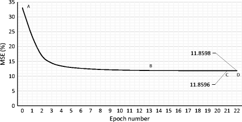

  

  The error curve of the ANN with parameters as above

• 2. Number of hidden layers: 1

• 3. Number of hidden neurons: 128

• 4. Y, the output vector size: 36

• 5. Batch size: 19

• 6. Learning rate η: 1.1

In Fig. 22, it can be seen that as the number of epochs increased, the errors the ANN made on the testing data decreased. At A, in the first epoch (epoch 0), the ANN made an error of 33%. At B, the error curve started to flat out at the 13th epoch. The ANN parameters are saved at the 21st epoch, since the error at epoch 22 is bigger that the error at epoch 21. The final MSE value at epoch 21 is 11.8596%, thus the ANN had an accuracy of 100 − 11.8596 = 88.15% when solving individual characters.

After the training process and saving ANN parameters for epoch 21, OCR could be executed automatically, or by running the ANN again with no command line inputs. The OCR part of the ANN worked by first reading in the saved ANN weights and biases of the trained ANN. Then, the ANN is constructed with the required amount of inputs, hidden neurons, and outputs. Given a licence plate with characters saved in a text file (“nn_inputs”) or represented by (10) as O _c , the ANN ran for the amount of characters (c _n ) that are present in O _c , identifying a character for each forward propagation iteration. To identify a single character, the input vector X is set to the first line of “nn_inputs”. Then forward propagation is applied, producing outputs at all neurons, and finally producing the output vector, Y. The output vector indicated a value of certainty for each character.

In testing, it is found that the ANN had an accuracy of 93% for licence plate characters (similar to individual character testing). The OCR part of the ANN is optimised by linking it to the web-hosted content component. The licence plate validation worked by checking vehicle access rights in a database table.

It should however be noted that recent studies incorporate the use of Sparse Graph Representation (SGR) algorithms such as shown in [26] and [28]. They can be used for classification or with noisy or large-scale data. Although we implemented a trivial neural network for this paper, SGR algorithms should definitely be considered for future implementations.

4.7 Web-hosted content

A web server is setup to host a website, and a MySQL database containing tables for vehicle access rights and system parameters. The website and database had a level of security [22] which required a user name and password for access. Various HTML, PHP and JSON scripts are implemented to accept requests from the website, as well as serve as a communication backbone for an Android application. The website and Android application is used to:

• 1. Open the gate.

• 2. Add or remove vehicle licence plates.

• 3. View system access logs.

• 4. Toggle a lockdown mode.

In addition to this, the functionality of push notifications are built into the Android application to offer the ability to notify the user about all system access attempts. The Google Firebase platform is used to achieve this. The software flow of the application can be seen in Fig. 23. The user interface of the application can be seen in Fig. 24, and examples of the push notification functionality can be seen in Fig. 25.

Fig. 23

Flow diagram for the flow of the Android software

Fig. 24

User interface of Android application

Fig. 25

Android application push notifications

4.8 Gate interface

The gate interface is designed as a stand-alone wireless module, which communicated with the main processor (Odroid) via two ESP8266 wireless transceiver modules (client and server). The client gate interface module consisted of an ESP8266 that is connected to the Odroid via the UART interface running at 115200 baud. Whenever a gate open request is received on the Odroid, the command is sent to the server gate interface via a wireless P2P link. An overview of the gate interface can be seen in Fig. 26, where the hardware of the gate interface is shown.

Fig. 26

Gate interface overview

Most gate motors on the market offer the functionality to be opened by an external device such as an indoor intercom. The motors are designed to have a terminal that if shorted to a common terminal, the gate will open. Using this knowledge, a gate interface circuit is designed and implemented as a stand-alone module to the main system (Odroid). We designed the gate interface to accept a command to open the gate over a wireless P2P connection [11] from the Odroid, and then open the gate as in the gate interface part of Fig. 26. The gate interface consisted of a ESP8266, a microcontroller [27], and a relay circuit. To open the gate the 8-byte validation code below was used.

$$\begin{array}{@{}rcl@{}} \begin{array}{llllllll} Code &= 10101010 \end{array} \end{array} $$

(38)

To open the gate, a transistor is used to activate a relay. Since the digital pin voltage of the microcontroller is 3.3 V, the same as the Odroid, the transistor and relay implementation of the ambient light sensor [33] and control circuitry is implemented and adapted for the gate interface. For the transistor [13], the values from (5) and (6) is used to calculate a base resistor (R _b = 11.41 kΩ). A protection diode (D _{p r o c} ) is also installed in parallel to the relay coil to protect the microcontroller and ESP8266 module. The gate interface module is powered using 12 V, since most gate motors have a 12 V backup battery. An LM317 voltage regulator is used to regulate the battery voltage, V _{b a t} = 12 V down to a regulated voltage, V _{r e g} = 3.3 V. The calculation for voltage regulation can be seen in (39), where the output resistor is chosen as R _{o u t} = 680 Ω, and the voltage adjust resistor is calculated as R _{a d j} = 1.12 kΩ.

$$\begin{array}{@{}rcl@{}} \begin{array}{llllllll} V_{reg} &= 1.25 \left( 1 + \frac{R_{out}}{R_{adj}} \right)\\ 3.3 &= 1.25 \left( 1 + \frac{680}{R_{adj}} \right)\\ R_{adj} &= 1.12\ k{\Omega} \end{array} \end{array} $$

(39)

The schematic of the server side gate interface can be seen in Fig. 27. The final gate interface PCB layout can be seen in Fig. 28. The enclosure of the gate interface can be seen in Fig. 29.

Fig. 27

Final schematic of gate interface circuitry (server)

Fig. 28

Populated PCB of server gate interface

Fig. 29

Server gate interface enclosure

4.9 Final system

The final implemented system and components can be seen in Fig. 30, where the main system containing the Odroid can be seen on the left, and the various sensors an the right.

Fig. 30

Final implemented system

5 Results

5.1 Proximity sensor

Using a tape measure, the line of sight of the proximity sensor was broken at intervals of 20 cm (using a piece of white paper). The output of the proximity sensor was measured on the digital multimeter and on the Odroid to test its maximum detection range. It was found that the proximity sensor could detect the presence of a vehicle within its designed range of 140 cm. More surprisingly, it could detect vehicles up to a maximum distance of 179 cm.

5.2 Ambient light sensor and control circuitry

The ambient light sensor is used to measure ambient light intensities, and if necessary, turn on an ambient light source. Within Table 3, measurements taken with a digital multimeter were compared to measurements in software.

Table 3 Ambient light sensor voltages

The ambient light was activated in dark to moderate light ambient conditions as expected. It was observed that the licence plates were readable, but vehicle headlights posed some problems regarding visibility in the night.

5.3 Gate interface

The gate interface was able to successfully communicate with the main system up to a distance of 40 m, and it was able to successfully integrate with existing gate motors on the market.

5.4 Neural network training

The trained ANN had an accuracy of 88.15% on the training data. In Fig. 22, the training curve of the ANN can be seen, where the final MSE and accuracy were achieved after 21 epochs.

5.5 Licence plate and character extraction, and character recognition

Licence plate and character extraction had individual accuracies of 87% and 97.6% respectively. It was found that licence plates in good (legal) conditions did not pose any problems for licence plate extraction and character extraction. It was found that illegally mounted and damaged plates made the licence plate and character extraction process more difficult. The camera that was used was cost-effective, although low light and colour representation was compromised. Due to this fact, difficulties were present in extracting characters in dark ambient conditions with the presence of vehicle head lights, as well as difficulties identifying all the characters in a Mpumalanga licence plate. Overall it was found that the ANN had an accuracy of 88.15% for recognising the computer font training characters, and 93% for identifying individual licence plate characters. Depending on the quality of an image, the ANN could mistake for example a “0” and an “O”, or an “1” and an “I”, thus an error correction algorithm was applied to the ANN, after which it could identify 100% of a licence plate’s characters, 80% of the time.

6 Future work

The system is designed to allow for future add-ons and improvements. It is believed that the system could function as an outdoor hub for IoT devices for instance outside a house. Since the system is able to open a security gate using an ANN to perform character recognition, it is suggested that facial recognition be implemented for future work to the project. Facial recognition could be used at smaller security gates to automate the entrance process of people.

It is also suggested to connect the system to existing CCTV feeds that may exist at shopping centres or business parks. using this suggested method, gate automation could be easily implemented at remote locations. In addition to this, video compression techniques can also be applied in order to save transmission bandwidth. As explained in [29,30,31] and [32], High Efficiency Video Coding (HEVC), a high coding efficiency standard can be used to accomplish this. It should be noted however that the HEVC video coding standard saves transmission bandwidth with the cost of greater computational overhead at both transmission ends.

To fully utilise the power of IoT, an iOS application could also be developed with the same control, monitor, and notification abilities as the Android application. With another important consideration being the lightweight messaging protocol MQTT with similar application such as [6]. Incorporating MQTT will ensure easy integration with existing home automation platforms.

7 Conclusion

Vehicle licence plates could successfully be validated using the ANN with an accuracy of 93% on identifying the individual characters of a licence plate, and 88.15% on identifying the individual characters from the training data set. The improved accuracy on the individual licence plate characters is due to the licence plate characters being of uniform nature, unlike the training data being of alternating computer fonts.

For the image processing, the final accuracies of the licence plate extraction and character extraction was 87% and 97.6% respectively, directly adversely effected by the quality of the captured images.

The proximity sensor achieved to detect objects for a range up to 179 cm with small variations due to the colour and texture of the objects to detect, whilst the ambient light sensor was able to differentiate between dark and light ambient lighting conditions.

The gate interface could connect to the main system with communication being reliable and without errors up to 40 m.

The implemented web-hosted content worked as designed to attribute to IoT principles with functionality to register and deregister vehicles, check system logs, open a gate, and toggle a system lockdown mode.

References

Ahmed A U, Masum T M, Rahman M M (2014) Design of an automated secure garage system using license plate recognition technique. Int J Intell Syst Appl 6 (2):22
Bovik A C (2011) Digital image processing. Tata McGraw Hill Education
Canny J (1986) A computational approach to edge detection. IEEE Trans Pattern Anal Mach Intell 8(6):679–698
Chang S L, Chen L S, Chung Y C, Chen S W (2004) Automatic license plate recognition. IEEE Trans Intell Transp Syst 5(1):42–53
Dedgaonkar S, Chandavale A, Sapkal A (2012) Survey of methods for character recognition. Int J Eng Innov Technol 1(5):180–189
Dhar P, Gupta P (2016) Intelligent parking cloud services based on iot using mqtt protocol. In: 2016 International conference on automatic control and dynamic optimization techniques (ICACDOT), pp 30–34
Fowler K R, Fowler K (1996) Electronic instrument design: architecting for the life cycle. Oxford University Press on Demand
Gilli M, Schumann E (2011) Numerical methods and optimization in finance. Academic Press
Hagan M T, Demuth H B, Beale M H, De Jesu̇s O (1996) Neural network design, 2nd edn. PWS Publishing Company, Boston
International Telecommunication Union (2002) Parameter values for the HDTV standards for production and international programme exchange BT Series Broadcasting service. Recommendation ITU-R BT.709-5, vol 5, pp 3–5
Jaco Prinsloo R M (2016) Accurate vehicle location system using rfid, an internet of things approach. Sensors MDPI 16(1):1–24
Jayalakshmi P, Kumar T R (2013) Automatic license plate recognition using computer vision for door opening. Int J Emerg Trends Electr Electron 4(2):65–68
Jaco Prinsloo R M (2016) Vehicle trajectory prediction based on hidden markov model. KSII Trans Internet Inf Sys 10(5):3150–3170
Kaur S (2013) Analysis of software engineering models for sorftware development and quality management. Int J Soft Comput Softw Eng 3(3):94–97
Mousa A (2012) Canny edge-detection based vehicle plate recognition. Int J Signal Process Image Process Pattern Recogn 5(3):1–8
Neto E C, Rebouċas E S, Moraes J L, Gomes S L, Filho P P R (2015) Development control parking access using techniques digital image processing and applied computational intelligence. Latin Amer Trans IEEE (Revista IEEE America Latina) 13(1):272–276
Nunes R (2004) A web-based approach to the specification and programming of home automation systems. In: Electrotechnical Conference, 2004. MELECON, 2004. Proceedings of the 12th IEEE Mediterranean, vol 2, pp 693–696
Ondrej M, Zboril V, Frantisek, Martin D (2007) Algorithmic and mathematical principles of automatic number plate recognition systems. Brno University of Technology, pp 20–22
Phillips D (1994) Image processing in C, vol 2. Citeseer
Rashid M M, Musa A, Rahman M A, Farahana N, Farhana A (2012) Automatic parking management system and parking fee collection based on number plate recognition. Int J Mach Learn Comput 2(2):93–98
Sergio F (2001) Design with operational amplifiers and analog integrated circuits, 3rd edn. McGraw-Hill Education
Tianhe Gong P C T C, Huang H (2016) Secure two party distance computation protocol based on privacy homomorphism and scalar product in wireless sensor networks. Tsinghua Sci Technol 21(2):385–396
Tu J V (1996) Advantages and disadvantages of using artificial neural networks versus logistic regression for predicting medical outcomes. J Clin Epidemiol 49:1225–1231
Van Heerden R (2002) Hidden Markov models for robust recognition of vehicle licence plates. South Africa, University of Pretoria
Wang C, Daneshmand M, Dohler M, Mao X, Hu R Q, Wang H (2013) Guest editorial - special issue on internet of things (IoT): architecture, protocols and services. IEEE Sensors J 13(10):3505–3508
Xu Y, Zhang D, Yang J, Yang J Y (2011) A two-phase test sample sparse representation method for use with face recognition. IEEE Trans Circ Syst Vid Technol 21(9):1255–1262
Xue Z, Du P, Li J, Su H (2016) Trackt: accurate tracking of rfid tags with mm-level accuracy using first-order taylor series approximation. AD Hoc Netw 53 (1):132–144
Xue Z, Du P, Li J, Su H (2017) Sparse graph regularization for hyperspectral remote sensing image classification. IEEE Trans Geosci Remote Sens 55(4):2351–2366
Yan C, Zhang Y, Xu J, Dai F, Li L, Dai Q, Wu F (2014) A highly parallel framework for hevc coding unit partitioning tree decision on many-core processors. IEEE Signal Process Lett 21(5):573–576
Yan C, Zhang Y, Xu J, Dai F, Zhang J, Dai Q, Wu F (2014) Efficient parallel framework for hevc motion estimation on many-core processors. IEEE Trans Circ Syst Video Technol 24(12):2077–2089
Yan C, Zhang Y, Dai F, Wang X, Li L, Dai Q (2014) Parallel deblocking filter for hevc on many-core processor. Electron Lett 50(5):367–368
Yan C, Zhang Y, Dai F, Zhang J, Li L, Dai Q (2014) Efficient parallel hevc intra-prediction on many-core processor. Electron Lett 50(11):805–806
Zhongqin Wang R W P L, Ye N (2016) Tmicroscope: behavior perception based on the slightest rfid tag motion. Elektronika ir Elektrotechnika 22(2):114–122
Zurada J M (1992) Introduction to artificial neural systems. West Publishing
Acknowledgements
This work is supported in part by the National Research Foundation, South Africa (grant numbers: IFR160118156967 and RDYR160404161474). The authors would like thank Mr. Arun Jose Cyril for editing revised version of this paper.
Author information
Authors and Affiliations
Corresponding author
Rights and permissions
About this article
Cite this article
Cowdrey, K., Malekian, R. Home automation - an IoT based system to open security gates using number plate recognition and artificial neural networks. Multimed Tools Appl 77, 20325–20354 (2018). https://doi.org/10.1007/s11042-017-5407-1
Received:
Revised:
Accepted:
Published:
Issue Date:
DOI: https://doi.org/10.1007/s11042-017-5407-1