
Abstract
We investigate the fundamental relation between entropy production rate and the speed of energy exchange between a system and baths in classical Markov processes. We establish the fact that quick energy exchange inevitably induces large entropy production in a quantitative form. More specifically, we prove two inequalities on instantaneous quantities: one is applicable to general Markov processes induced by heat baths, and the other is applicable only to systems with the local detailed-balance condition but is stronger than the former one. We demonstrate the physical meaning of our result by applying to some specific setups. In particular, we show that our inequality is tight in the linear response regime.
Notes
Here, one may feel that for a cyclic process of a macroscopic heat engine the initial and final states are considered to be the same only in the macroscopic sense, and its microscopic probability distribution is not expected to be the same (i.e., \(p_{w,0}=p_{w,\tau }\) is a non-realistic assumption for macroscopic engines). However, fortunately, what we have utilized in our derivation is only the following weaker conditions that both the Shannon entropy and the energy expectation value are the same between the states at \(t=0\) and \(t=\tau \):
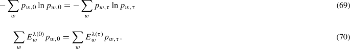
Hence, if the Shannon entropy and energy do not change between the initial and the final states, our trade-off inequality (73) is still valid even when other microscopic details are changed between the initial and the final states.
This entropy is defined in thermodynamic sense. Because the entropy production in stochastic thermodynamics contains the entropy increase of baths as in the thermodynamic sense and the Shannon entropy of the systems is assumed to be invariant, this definition of \({\varDelta }S\) is consistent with the definition of entropy production in stochastic thermodynamics.

References
Evans, D.J., Cohen, E.G.D., Morriss, G.P.: Probability of second law violations in shearing steady states. Phys. Rev. Lett. 71, 2401 (1993)
Kurchan, J.: Fluctuation theorem for stochastic dynamics. J. Phys. A Math. Gen. 31, 3719 (1998)
Jarzynski, C.: Hamiltonian derivation of a detailed fluctuation theorem. J. Stat. Phys. 98, 77 (2000)
Mahan, G.D., Sofo, J.O.: The best thermoelectric. Proc. Natl Acad. Sci. U.S.A. 93, 7436 (1996)
Mahan, G.D., Sales, B., Sharp, J.: Thermoelectric materials: New approaches to an old problem. Phys. Today 50, 42 (1997)
Majumdar, A.: Thermoelectricity in semiconductor nanostructures. Science 303, 777 (2004)
Snyder, G.J., Toberer, E.R.: Complex thermoelectric materials. Nat. Mater. 7, 105 (2008)
Casati, G., Mejía-Monasterio, C., Prosen, T.: Incresing thermoelectric efficiency: a dynamic systems approach. Phys. Rev. Lett. 101, 016601 (2008)
Shiraishi, N.: Attainability of Carnot efficiency with autonomous engines. Phys. Rev. E 92, 050101 (2015)
Tajima, H., Hayashi, M.: Finite-size effect on optimal efficiency of heat engines. Phys. Rev. E 96, 012128 (2017)
Shiraishi, N.: Stationary engines in and beyond the linear response regime at the Carnot efficiency. Phys. Rev. E 95, 052128 (2017)
Benenti, G., Casati, G., Saito, K., Whitney, R.S.: Fundamental aspects of steady-state conversion of heat to work at the nanoscale. Phys. Rep. 694, 1 (2017)
Benenti, G., Saito, K., Casati, G.: Thermodynamic bounds on efficiency for systems with broken time-reversal symmetry. Phys. Rev. Lett. 106, 230602 (2011)
Allahverdyan, A.E., Hovhannisyan, K.V., Melkikh, A.V., Gevorkian, S.G.: Carnot cycle at finite power: attainability of maximal efficiency. Phys. Rev. Lett. 111, 050601 (2013)
Campisi, M., Fazio, R.: The power of a critical heat engine. Nat. Commun. 7, 11895 (2016)
Ponmurugan, M.: Attainability of maximum work and the reversible efficiency from minimally nonlinear irreversible heat engines. arXiv:1604.01912 (2016)
Polettini, M., Esposito, M.: Carnot efficiency at divergent power output. Europhys. Lett. 118, 40003 (2017)
Johnson, C.V.: Approaching the Carnot limit at finite power: an exact solution. Phys. Rev. D 98, 026008 (2018)
Curzon, F.L., Ahlborn, B.: Efficiency of a Carnot engine at maximum power output. Am. J. Phys. 43, 22 (1975)
Andresen, B., Berry, R.S., Ondrechen, M.J., Salamon, P.: Thermodynamics for processes in finite time. Acc. Chem. Res. 17, 266 (1984)
Sothmann, B., Büttiker, M.: Magnon-driven quantum-dot heat engine. Europhys. Lett. 99, 27001 (2012)
Brandner, K., Saito, K., Seifert, U.: Strong bounds on Onsager coefficients and efficiency for three-terminal thermoelectric transport in a magnetic field. Phys. Rev. Lett. 110, 070603 (2013)
Brandner, K., Seifert, U.: Multi-terminal thermoelectric transport in a magnetic field: bounds on Onsager coefficients and efficiency. New J. Phys. 15, 105003 (2013)
Balachandran, V., Benenti, G., Casati, G.: Efficiency of three-terminal thermoelectric transport under broken time-reversal symmetry. Phys. Rev. B 87, 165419 (2013)
Brandner, K., Seifert, U.: Bound on thermoelectric power in a magnetic field within linear response. Phys. Rev. E 91, 012121 (2015)
Yamamoto, K., Entin-Wohlman, O., Aharony, A., Hatano, N.: Efficiency bounds on thermoelectric transport in magnetic fields: the role of inelastic processes. Phys. Rev. B 94, 121402 (2016)
Brandner, K., Saito, K., Seifert, U.: Thermodynamics of micro-and nano-systems driven by periodic temperature variations. Phys. Rev. X 5, 031019 (2015)
Proesmans, K., Van den Broeck, C.: Onsager coefficients in periodically driven systems. Phys. Rev. Lett. 115, 090601 (2015)
Proesmans, K., Cleuren, B., Van den Broeck, C.: Linear stochastic thermodynamics for periodically driven systems. J. Stat. Mech. P023202 (2016)
Pietzonka, P., Seifert, U.: Universal trade-off between power, efficiency and constancy in steady-state heat engines. Phys. Rev. Lett. 120, 190602 (2018)
Sekimoto, K., Sasa, S.-I.: Complementarity relation for irreversible process derived from stochastic energetics. J. Phys. Soc. Jpn. 66, 3326 (1997)
Aurell, E., Gawȩdzki, K., Mejía-Monasterio, C., Mohayaee, R., Muratore-Ginanneschi, P.: Refined second law of thermodynamics for fast random processes. J. Stat. Phys. 147, 487 (2012)
Raz, O., Subaşı, Y., Pugatch, R.: Geometric heat engines featuring power that grows with efficiency. Phys. Rev. Lett. 116, 160601 (2016)
Barato, A.C., Seifert, U.: Thermodynamic uncertainty relation for biomolecular processes. Phys. Rev. Lett. 114, 158101 (2015)
Gingrich, T.R., Horowitz, J.M., Perunov, N., England, J.L.: Dissipation bounds all steady-state current fluctuations. Phys. Rev. Lett. 116, 120601 (2016)
Gingrich, T.R., Rotskoff, G.M., Horowitz, J.M.: Inferring dissipation from current fluctuations. J. Phys. A Math. Theor. 50, 184004 (2017)
Pietzonka, P., Ritort, F., Seifert, U.: Finite-time generalization of the thermodynamic uncertainty relation. Phys. Rev. E 96, 012101 (2017)
Horowitz, J.M., Gingrich, T.R.: Proof of the finite-time thermodynamic uncertainty relation for steady-state currents. Phys. Rev. E 96, 020103 (2017)
Dechant, A., Sasa, S.: Current fluctuations and transport efficiency for general Langevin systems. J. Stat. Mech. 063209 (2018)
Dechant, A., Sasa, S.: Fluctuation-response inequality out of equilibrium. arXiv:1804.08250 (2018)
Shiraishi, N., Saito, K., Tasaki, H.: Universal trade-off relation between power and efficiency for heat engines. Phys. Rev. Lett. 117, 190601 (2016)
Cover, T.M., Thomas, J.A.: Elements of Information Theory. Wiley, New York (1991)
Taneja, I.J.: Bounds on triangular discrimination, harmonic mean and symmetric chi-square divergences. arXiv:math/0505238 (2005)
Shiraishi, N., Sagawa, T.: Fluctuation theorem for partially masked nonequilibrium dynamics. Phys. Rev. E 91, 012130 (2015)
Shiraishi, N., Ito, S., Kawaguchi, K., Sagawa, T.: Role of measurement-feedback separation in autonomous Maxwell’s demons. New J. Phys. 17, 045012 (2015)
Shiraishi, N., Matsumoto, T., Sagawa, T.: Measurement-feedback formalism meets information reservoirs. New J. Phys. 18, 013044 (2016)
Shiraishi, N., Saito, K.: Incompatibility between Carnot efficiency and finite power in Markovian dynamics. arXiv:1602.03645 (2016)
Van Kampen, N.G.: Stochastic Process in Physics and Chemistry, 3rd edn. Elsevier, Amsterdam (2007)
Breuer, H.-P., Petruccione, F.: The Theory of Open Quantum Systems. Oxford University Press, Oxford (2002)
Shiraishi, N., Tajima, H.: Efficiency versus speed in quantum heat engines: rigorous constraint from Lieb–Robinson bound. Phys. Rev. E 96, 022138 (2017)
Perarnau-Llobet, M., Wilming, H., Riera, A., Gallego, R., Eisert, J.: Strong coupling corrections in quantum thermodynamics. Phys. Rev. Lett. 120, 120602 (2018)
Funo, K., Shiraishi, N., Saito, K.: Speed limit for open quantum systems. arXiv:1810.03011 (2018)
Brandner, K., Hanazato, T., Saito, K.: Thermodynamic bounds on precision in ballistic multi-terminal transport. Phys. Rev. Lett. 120, 090601 (2018)
Macieszczak, K., Brandner, K., Garrahan, J.P.: Unified thermodynamic uncertainty relations in linear response. Phys. Rev. Lett. 121, 130601 (2018)
Shiraishi, N.: Finite-time thermodynamic uncertainty relation do not hold for discrete-time Markov process. arXiv:1706.00892 (2017)
Proesmans, K., Van den Broeck, C.: Discrete-time thermodynamic uncertainty relation. Europhys. Lett. 119, 20001 (2017)
Shiraishi, N., Funo, K., Saito, K.: Speed limit for classical stochastic processes. Phys. Rev. Lett. 121, 070601 (2018)
Siegel, A.: Differential-operator approximations to the linear Boltzmann equation. J. Am. Phys. 1, 378 (1960)
Van den Broeck, C., Kawai, R., Meurs, P.: Microscopic analysis of a thermal Brownian motor. Phys. Rev. Lett. 93, 090601 (2004)
Fruleux, A., Kawai, R., Sekimoto, K.: Momentum transfer in nonequilibrium steady states. Phys. Rev. Lett. 108, 160601 (2012)
Seifert, U.: Stochastic thermodynamics, fluctuation theorems, and molecular machines. Rep. Prog. Phys. 75, 126001 (2012)
Acknowledgements
We are grateful to Hal Tasaki for fruitful discussion. He was a co-author in the joint work [41], and contributed to deriving several relations. NS was supported by Grant-in-Aid for JSPS Fellows JP17J00393. KS was supported by JSPS Grants-in-Aid for Scientific Research (No. JP25103003, JP16H02211 and JP17K05587).
Author information
Authors and Affiliations
Corresponding author
Appendices
Appendix A: Analysis with Linear Irreversible Thermodynamics
In this appendix, we clarify the fact that if time-reversal symmetry is broken the linear irreversible thermodynamics does not prohibit the existence of a heat engine with the Carnot efficiency at finite power [13]. We consider a stationary system with two kinds of flux \(J_1\) and \(J_2\) with corresponding thermodynamic forces \(X_1\) and \(X_2\). We set \(J_2\) to heat flux and \(X_2:=1/T_L-1/T_H\), \(J_1\) to another flux which flows against the thermodynamic force \(X_1\) (i.e., \(X_1J_1\le 0\) and \(X_2J_2\ge 0\)). The power and efficiency are given by \(\dot{W}:=-X_1J_1T\) and \(\eta :=-X_1J_1T/J_2\).
We consider a system with a magnetic field B. In this system, the linear expansion of the flux J is written as
where L is the Onsager matrix. The Onsager reciprocity relation tells \(L_{12}(B)=L_{21}(-B)\), and in general \(L_{12}(B)\ne L_{21}(B)\). In the remainder of this appendix, since we consider only systems with a magnetic field B, we omit the parameter B. The entropy production rate \(\dot{S}:=J_1X_1+J_2X_2\) is calculated as
Because the second law of thermodynamics claims \(\dot{S}\ge 0\) for any \(X_1\) and \(X_2\), by setting \(X_1=-(L_{12}+L_{21})X_2/2L_{11}\), we find that the coefficient of the second term of Eq. (A.3) is nonnegative:
This condition suggests that the entropy production rate is bounded by a quadratic term:
We now investigate the condition for the Carnot efficiency \(\dot{S}=0\). We first consider the case with time-reversal symmetry (i.e., \(L_{12}=L_{21}\)). In this case, Eq. (A.5) reduces to
which looks very similar to Eq. (38), and clearly shows that the Carnot efficiency \(\dot{S}=0\) is achievable only when power is zero: \(\left| J_1\right| =0\).
We next consider the case without time-reversal symmetry. Equation (A.3) suggests that \(\dot{S}=0\) holds if and only if the following two conditions
are satisfied simultaneously. Then, if \(L_{12}\ne L_{21}\), for any L satisfying \(L_{22}-{(L_{12}+L_{21})^2}/{4L_{11}}=0\) and any nonzero \(X_2\), there exists nonzero \(X_1=-{(L_{21}+L_{12})X_2}/{2L_{11}}\) satisfying Eq. (A.8). We note that \(X_2\ne 0\) and \(L_{21}-L_{12}\ne 0\) directly imply finite power: \(J_1\ne 0\). Since the second condition (A.8) can be always satisfied by setting nonzero \(X_1\) and \(X_2\) properly as long as \(L_{12}\ne L_{21}\), the remaining question is whether the first condition (A.7) is realizable under \(L_{12}\ne L_{21}\). However, within the framework of the linear irreversible thermodynamics, there is no a priori reason to exclude the possibility of \(L_{22}-{(L_{12}+L_{21})^2}/{4L_{11}}=0\) with \(L_{12}\ne L_{21}\).
This clearly shows that finite power and the Carnot efficiency is compatible under a magnetic field. We, however, should note that the above analysis only shows that the linear irreversible thermodynamics does not formally exclude the possibility of a heat engine with the Carnot efficiency at finite power, and does not show that there indeed exists such a heat engine. In fact, as seen in the main part of this paper, by taking into account microscopic details of the system, we find that the Carnot efficiency and finite power are incompatible.
Appendix B: Discretization and Continuum Limit of Kramers Equation and Hamilton’s Equation
In this appendix, we provide the detailed procedure of the discretization and continuum limit for continuous systems, which is briefly discussed in Sect. 2.1.2. Same as Sect. 2.1.2, we consider a Markov process of a single particle in one-dimensional continuous space described by the following Kramers equation:
where x and p are the position and momentum of the particle. We remark that stochastic Markov processes obtained through the system size expansion always take this form of equation [48].
The right-hand side of Eq. (B.1) is decomposed into the Hamiltonian part
and the dissipative part
The former is equivalent to Hamilton’s equation:
The latter is equivalent to the following Langevin equiation:
Here, \(\xi (t)\) represents the white Gaussian noise. The first term represents the viscous resistance, and the second term represents stochastic thermal noise. The equivalence of the Langevin equation and the Fokker-Planck equation is shown in many textbooks [48].
We first consider the discretized transition matrix corresponding to the dissipative part. The transition matrix from a state with momentum p to \(p\pm \varepsilon \) is given by Eq. (11), which reappears below:
We shall show that this transition rate indeed reproduces the dissipative part (B.3). Expanding the transition matrix in \(\varepsilon \) as
with \(A:=\gamma /\beta \varepsilon ^2\), the master equation with Eq. (B.7) becomes
Taking \(\varepsilon \rightarrow 0\) limit, we recover the Kramers equation:
Hence, the discretization with the transition rate (B.7) indeed reproduces the time-evolution of (B.3).
We next consider the discretized transition matrix corresponding to the Hamiltonian part. This discretization draws the \(p-x\) phase space as the \(\varepsilon \times \varepsilon '\) lattice. A single state is determined by a pair of position and momentum, (x, p). Supposing \(p>0\) and \(F(x,p)>0\), we set the transition matrix of (x, p) as Eqs. (9) and (10), which reappear below:
We remark that the inverse transitions of the above transitions do not occur (i.e., \(R_{ (x,p),(x,p+\varepsilon )}=0\) and \(R_{(x,p),(x+\varepsilon ',p)}=0\)). The master equation reads
whose continuum limit \(\varepsilon , \varepsilon ' \rightarrow 0\) reproduces the Liouville operator
Hence, the discretization with the transition rates (B.12) and (B.13) indeed reproduce the time-evolution of (B.2).
Appendix C: Proof of Lemma 1
We recast the Lemma 1:
with \(c_0=8/9\). In the following, we shall show the proof of this inequality.
Proof
We first show an inequality
for any \(a,b >0\). This inequality is equivalent to
with \(u:=b/a\). Since \(h(1)=0\), it is enough to show that the derivative of h(u)
satisfies \(h'(u)\ge 0\) for \(u\ge 1\) and \(h'(u)\le 0\) for \(0<u\le 1\).
We first show \(h'(u)\le 0\) for \(0<u\le 1\). In \(0<u\le 1\), both
and
hold due to \(c_0<1\), which directly implies \(h'(u)\le 0\).
We next show \(h'(u)\ge 0\) for \(u\ge 1\). In \(u\ge 1\), both
and
hold due to \(c_0\le 8/9\), which directly implies \(h'(u)\ge 0\).
Combining them, we obtain the inequality (C.2), whose sum over all i is equivalent to the desired inequality (43):
\(\square \)
Appendix D: Proof of Lemma 2
We recast the Lemma 2 below:
In the following, we shall show the proof of this inequality.
Proof
Due to the symmetry, we set \(a>b\) without loss of generality. (In case of \(a=b\), Eq. (D.1) is obviously satisfied.) The inequality (D.1) is equivalent to
This relation directly follows from the downward-convexity of the function 1 / x:
\(\square \)
Appendix E: Inequality on Relative Entropy
We derived an inequality between relative entropy and triangular discrimination (43) in Sect. 4.1.1. The obtained inequality is better than the existing one [43]:
However, our coefficient \(c_0=8/9\) is still not the best one. We here seek the best coefficient.
The crucial relation in the derivation is
We consider the maximum of c satisfying the above inequality for any \(a,b>0\). As shown in Appendix C, this inequality is equivalent to
with \(u>0\). The local minimum of h(u) for \(c>8/9\) is calculated as
We denote the second solution by \(u^*(c)\). Because \(h(1)=0\), \(h(u^*(c))\ge 0\) is the necessary and sufficient condition for \(h(u)\ge 0\). The relation \(h(u^*(c))\ge 0\) is solved numerically as
whose right-hand side is the best coefficient for the inequality between relative entropy and triangular discrimination:
We remark that the above coefficient is tightest because a nontrivial pair of probability distributions \(p_1=1/(1+u^*(c^*))\), \(p_2=u^*(c^*)/(1+u^*(c^*))\), \(q_1=u^*(c^*)/(1+u^*(c^*))\), \(q_2=1/(1+u^*(c^*))\) achieves its equality.
Appendix F: Finiteness of \(\varvec{\varTheta }\)
In this appendix, we show that \(\varTheta \) is finite under some physically-plausible assumptions.
1.1 Upper Bound of \(\varvec{\varTheta }^{(1)}\)
We here derive some upper bounds of \(\varTheta ^{(1)}\). We first bound \(\varTheta _\mu ^{(1)}\) defined in Eq. (54) as
Here, \(R_\mathrm{max}\) is the maximum of the absolute value of the diagonal elements of the transition matrix (i.e., \(|R_{ww}^{\mu , \lambda (t)}|\le R_\mathrm{max}\) for all w and t), and \(\left[ \frac{d}{dt}\right] _\mu \) represents time derivative in case that the time evolution is induced only by \(R^{\mu , \lambda (t)}\). In the above calculation, we used the fact that \(R^{\mu , \lambda (t)}\) keeps the distribution \(p_{w^{-i}}\). Because the fluctuation of the energy of the ith particle \(\langle ({\varDelta }E_w^{\mu , \lambda (t)})^2\rangle _{t,w^{-i}}\) and its time derivative are expected to be finite in physical systems, the above relation implies that \(\varTheta ^{(1)}_\mu \) is finite if the diagonal elements of the transition matrix is bounded above.
In some cases, we can obtain the upper bound of \(\varTheta ^{(1)}_\mu \) even though the diagonal elements of the transition matrix is unbounded. To treat this situation, we again consider a system where only the particle i is movable and other particles are fixed at \(w^{-i}\). We introduce a quantity \(E_w^{i,\lambda (t)}\) which is the energy of the particle i under the condition that other particles are fixed at \(w^{-i}\). Note that \(E_w^{i,\lambda (t)}=O(1)\) with respect to the number of particles M. We now state some requirements on the system. First, we assume that the conditional probability distribution decays exponentially with energy: \(p_{w^i,t|w^{-i}} \le C_1\cdot e^{-a E_w^{i,\lambda (t)}}\) with constants \(C_1\) and a. This condition means that the probability distribution is not so far from a canonical distribution. We also assume that both the diagonal term of the transition matrix and the number of states of the ith particle below a certain energy \(\Omega _{w^i|w^{-i}} (E)\) increase only polynomially with respect to energy: \(|R_{ww}^{\mu , \lambda (t)}|\le C_2 (E_w^{i,\lambda (t)})^b\) and \(\Omega _{w^i|w^{-i}} (E)\le C_3 E^c\) with constants \(C_2\), \(C_3\), b and c, where \(\mu =(i,\nu )\). These conditions are expected to be satisfied in small systems with a finite number of particles including master-Boltzmann systems [58,59,60]. Under the aforementioned assumptions, \(\varTheta _\mu ^{(1)}\) is bounded above as
where the integral \(\int _0^\infty dx x^{2+c+b}e^{-ax}\) is obviously finite.
1.2 Thermodynamic Limit
The obtained inequalities (38) and (41) are still meaningful even in the thermodynamic limit. In other words, the inequalities provide a nontrivial prediction for macroscopic systems.
The inequalities contain three terms, the heat current \(J^\mathrm{q}\), the entropy production rate \(\dot{\sigma }\), and the coefficient \(\varTheta \). The former two terms are proportional to the system size V or the particle number M (More precisely, \(J^\mathrm{q}_\nu \), \(\hat{\sigma }\) and \(\varTheta \) are proportional to the volume of the region interacting with baths). We first consider the case of \(\varTheta =\varTheta ^{(2)}\). Because the number of states \(w'\) satisfying \(R_{w'w}\ne 0\) is proportional to M with fixed \(w=(w^1, \ldots ,w^M)\) and \((E_w-E_{w'})^2=O(1)\) is independent of M, \(\varTheta ^{(2)}\) is also proportional to M. We next confirm that \(\varTheta ^{(1)}\) is proportional to M. A single particle energy fluctuation \(({\varDelta }E_w^{\mu , \lambda (t)})^2\) defined in Eq. (40) is independent of M, which leads to \(\varTheta ^{(1)}_\mu =O(1)\). Then, since \(\varTheta ^{(1)}\) is the summation of it over \(\mu \), \(\varTheta ^{(1)}\) is proportional to M. We remark that because \(C_1=O(1/M)\), \(C_2=O(1)\), and \(C_3=O(M)\), the upper bound (F.2) also scales in proportion to M.
We note that \(\varTheta ^{(1)}\) is proportional to M because we did not employ the energy fluctuation of the whole system \({\varDelta }E_w^{\lambda (t)}:=E_w^{\lambda (t)}-\left\langle E\right\rangle _t\) itself, but to decompose it into the contribution from each particle in the definition of \(\varTheta ^{(1)}\). In fact, if we define \(\varTheta '\) by using \({\varDelta }E_w^{\lambda (t)}\) as
then (although the inequality \(\sum _\nu |J^\mathrm{q}_\nu | \le \sqrt{\varTheta ' \dot{\sigma }}\) still holds) this coefficient \(\varTheta '\) is proportional to \(M^2\). This is because the energy fluctuation of the whole system \({\varDelta }E_w^{\lambda (t)}\) has variance of order \(O(\sqrt{M})\). In this case, the inequality in the thermodynamic limit gives no information more than the second law of thermodynamics.
Appendix G: Extension of Eq. (86) to the Case of Finite Time Interval
Using the techniques that we have introduced, we can derive a similar but still different relation to the thermodynamic uncertainty relation. To this end, we consider a process in a finite-time interval \(0\le t\le \tau \) in stationary state with the local detailed-balance condition. Owing to the local detailed-balance condition, the entropy production rate is written as
We denote a single trajectory of time evolution in \(0\le t\le \tau \) by \(\varGamma \) and its time-reversal by \(\varGamma ^\dagger \). We also denote the probability density for the realization of \(\varGamma \) by \(P(\varGamma )\). The average of a stochastic variable is denoted by \(\left\langle \cdot \right\rangle \). It is well known that the total entropy production \(\varSigma :=\int _0^\tau dt \dot{\sigma }(t) =\tau \dot{\sigma }\) is written as [61]
Let \(X(\varGamma )\) be a time-asymmetric stochastic variable (i.e., \(X(\varGamma )=-X(\varGamma ^\dagger )\)), which includes any current of a conserved quantity. Then, X satisfies the following theorem:
Theorem 5
In a Markov process with finite time interval \(\tau \), we have
Here, we normalize the Boltzmann constant to unity.
Proof
We employ the same technique as the derivation of Eq. (41). With noting \(\int d\varGamma X(\varGamma )P(\varGamma )=-\int d\varGamma X(\varGamma ^\dagger )P(\varGamma )\) due to the time-asymmetric property of X, we transform \(\left| \left\langle X\right\rangle \right| ^2\) as
In a similar manner to Eq. (50), we have the following expression of the entropy production:
Finally, inserting the following relation
into Eq. (G.4), we arrive at the desired inequality:
\(\square \)
Appendix H: Efficiency of Thermoelectric Transport
We here briefly see how to define efficiency in a stationary thermoelectric transport system considered in Sect. 7.2. Same as Sect. 7.2, we consider two heat-particle baths with inverse temperatures and chemical potentials \(\beta _1, \mu _1\) and \(\beta _2, \mu _2\), respectively. We set \(\beta _1<\beta _2\), \(\mu _1<\mu _2\). The heat and particle currents from the bath 1 to 2 are denoted by \(J^\mathrm{q}\) and \(J^\mathrm{n}\), both of which we assume positive. Namely, the particle current \(J^\mathrm{n}\) flows against chemical potential gradient, which we regard as work.
In a cyclic process, efficiency is defined as \(W/Q_\mathrm{H}\) with \(Q_\mathrm{H}\) as heat absorption from the hot bath. We now define the counterpart of \(Q_\mathrm{H}\) in thermoelectric transport. Because particles themselves have their own energy in the form of chemical potential, we subtract this from heat current and regard \(J^\mathrm{q}-\mu _1J^\mathrm{n}\) as the counterpart of \(Q_\mathrm{H}\). Thus, we define efficiency in thermoelectric transport as
where we defined \({\varDelta }\mu :=\mu _2-\mu _1>0\) and assumed \(J^\mathrm{q}-\mu _1J^\mathrm{n}>0\).
We now confirm that the efficiency is indeed bounded by the Carnot efficiency
The above inequality is equivalent to
which is transformed into the nonnegativity of entropy production rate
Appendix I: Failure of Finite-Time Thermodynamic Uncertainty Relation in Relaxation Process
We show that the thermodynamic uncertainty relation \(\left\langle {\varDelta }X^2\right\rangle \varSigma \ge 2\left\langle X \right\rangle ^2\) holds only in stationary system, and cannot be extended to relaxation processes with time-independent transition matrix satisfying local detailed-balance condition.
Consider a stochastic process on two states \(w\in \{ 1,2\}\) with the same energy. The transition matrix thus satisfies \(R_{12}=R_{21}\). We set X as time integration of probability current from 1 to 2. Suppose that the initial distribution at \(t=0\) is \(p_1(0)=1\) and \(p_2(0)=0\), and consider the long time limit \(t\rightarrow \infty \), where the distribution relaxes to equilibrium distribution \(p_1(\infty )=p_2(\infty )=1/2\).
Straightforward calculation tells
Hence, \(\left\langle {\varDelta }X^2\right\rangle \varSigma =(\ln 2)/4< 1/4\) and \(2\left\langle X \right\rangle ^2 =1/2\), which obviously violates the extended thermodynamic uncertainty relation in relaxation processes.
Rights and permissions
About this article

Cite this article
Shiraishi, N., Saito, K. Fundamental Relation Between Entropy Production and Heat Current. J Stat Phys 174, 433–468 (2019). https://doi.org/10.1007/s10955-018-2180-0
Received:
Accepted:
Published:
Issue Date:
DOI: https://doi.org/10.1007/s10955-018-2180-0