Nonintersecting Brownian Motions on the Half-Line and Discrete Gaussian Orthogonal Polynomials

Abstract

We study the distribution of the maximal height of the outermost path in the model of N nonintersecting Brownian motions on the half-line as N→∞, showing that it converges in the proper scaling to the Tracy-Widom distribution for the largest eigenvalue of the Gaussian orthogonal ensemble. This is as expected from the viewpoint that the maximal height of the outermost path converges to the maximum of the Airy₂ process minus a parabola. Our proof is based on Riemann-Hilbert analysis of a system of discrete orthogonal polynomials with a Gaussian weight in the double scaling limit as this system approaches saturation. We consequently compute the asymptotics of the free energy and the reproducing kernel of the corresponding discrete orthogonal polynomial ensemble in the critical scaling in which the density of particles approaches saturation. Both of these results can be viewed as dual to the case in which the mean density of eigenvalues in a random matrix model is vanishing at one point.

Appendices

Appendix A: Proof of Lemmas 2.1 and 3.1

The proofs of Lemmas 2.1 and 3.1 are based on the following estimate of the rate of convergence of a Riemann sum, which is slightly sharper than the a priori rate of O(ε).

Lemma A.1

Let f(x ₁,…,x _n ) be an analytic function of n variables. Let the functions A _k (x ₁,…,x _n ) be defined recursively via

$$ A_{k}(x_1,\dots,x_n)=\sum _{j=1}^n \frac{\partial }{\partial {x}_j} A_{k-1}(x_1,\dots ,x_n), \qquad A_0 = f. $$

(A.1)

Suppose that

(A.2)

Then as ε→0,

$$ \int\cdots\int_{\mathbb {R}^n} f(x_1, \dots, x_n)\, dx_1 \cdots dx_n-\varepsilon ^n\sum _{x_1, \dots, x_n \in \varepsilon \mathbb {Z}}f(x_1, \dots, x_n)=O \bigl(\varepsilon ^4\bigr). $$

(A.3)

Proof

A multi-integral my be estimated by writing

(A.4)

Expanding each integrand on the RHS as a Taylor series and integrating term by term, this becomes

$$ \sum_{x_1, \dots, x_n \in \varepsilon \mathbb {Z}} \biggl[\varepsilon ^n f+ \frac{A_1}{2}\varepsilon ^{n+1}+\frac{A_2}{6}\varepsilon ^{n+2}+ \frac{A_3}{24}\varepsilon ^{n+3}+O\bigl(\varepsilon ^{n+4}\bigr) \biggr], $$

(A.5)

where

$$ f\equiv f(x_1,\dots,x_n), \qquad A_k\equiv A_j(x_1, \dots, x_n). $$

(A.6)

Thus the error in the Riemann sum is given by

$$ \begin{aligned}[b] & \int\cdots \int_{\mathbb {R}^n} f\, dx_1 \cdots dx_n-\sum_{x_1, \dots, x_n \in \varepsilon \mathbb {Z}} \varepsilon ^n f \\ &\quad =\varepsilon ^n \sum_{x_1, \dots, x_n \in \varepsilon \mathbb {Z}} \biggl[\frac{A_1}{2}\varepsilon +\frac{A_2}{6}\varepsilon ^{2}+ \frac{A_3}{24}\varepsilon ^{3}+O\bigl(\varepsilon ^{4}\bigr) \biggr] \\ &\quad = \biggl(\varepsilon ^n \sum_{x_1, \dots, x_n \in \varepsilon \mathbb {Z}} A_1 \biggr)\frac{\varepsilon }{2}+ \biggl(\varepsilon ^n \sum _{x_1, \dots, x_n \in \varepsilon \mathbb {Z}} A_2 \biggr)\frac{\varepsilon ^2}{6} \\ &\qquad{}+ \biggl(\varepsilon ^n \sum_{x_1, \dots, x_n \in \varepsilon \mathbb {Z}} A_3 \biggr)\frac{\varepsilon ^3}{24}+O\bigl(\varepsilon ^4\bigr). \end{aligned} $$

(A.7)

If (A.2) holds, then by the same argument,

$$ \begin{aligned}[c] \varepsilon ^n\sum _{x_1, \dots, x_n \in \varepsilon \mathbb {Z}} A_1(x_1, \dots, x_n)&=- \biggl(\varepsilon ^n \sum_{x_1, \dots, x_n \in \varepsilon \mathbb {Z}} A_2 \biggr)\frac{\varepsilon }{2}- \biggl(\varepsilon ^n \sum _{x_1, \dots, x_n \in \varepsilon \mathbb {Z}} A_3 \biggr)\frac{\varepsilon ^2}{6}+O \bigl(\varepsilon ^3\bigr), \\ \varepsilon ^n\sum_{x_1, \dots, x_n \in \varepsilon \mathbb {Z}} A_2(x_1, \dots, x_n)&=- \biggl(\varepsilon ^n \sum _{x_1, \dots, x_n \in \varepsilon \mathbb {Z}} A_3 \biggr)\frac{\varepsilon }{2}+O\bigl( \varepsilon ^2\bigr), \end{aligned} $$

(A.8)

and (A.7) can be written as

(A.9)

 □

Let us first apply this result to the proof of Lemma 3.1. By rescaling we can write (1.34) as

(A.10)

where

$$ \varepsilon =\pi\sqrt{\frac{r}{2n}}. $$

(A.11)

We have here an explicit prefactor times a Riemann sum for the function

$$ f(x_1, \dots, x_n)=\prod_{1\le j < k \le n} (x_k -x_j)^2 \exp \Biggl\{ -\sum _{j=1}^n x_j^2 \Biggr\}, $$

(A.12)

which is exactly the integrand in (1.56). One may easily check then that

$$ \begin{aligned}[c] A_1(x_1, \dots, x_n)&=-2(x_1+\cdots+x_n)f(x_1, \dots, x_n), \\ A_2(x_1, \dots, x_n)&=2f(x_1, \dots, x_n) \bigl(2(x_1+\cdots+x_n)^2-n \bigr) \\ &=-2 \bigl(A_1(x_1, \dots, x_n) (x_1+\cdots+x_n)+nf(x_1, \dots,x_n) \bigr). \end{aligned} $$

(A.13)

It is easy to see that A ₁ has the symmetry A ₁(x ₁,…,x _n )=−A ₁(−x ₁,…,−x _n ), from which it follows that

$$ \int\cdots\int_{\mathbb {R}^n} A_1(x_1, \dots, x_n)\, dx_1 \cdots dx_n=0. $$

(A.14)

It is a simple exercise to integrate by parts to see that

$$ \int\cdots\int_{\mathbb {R}^n} A_2(x_1, \dots, x_n) \,dx_1 \cdots dx_n=0. $$

(A.15)

It then follows that as r→0,

$$ \begin{aligned}[b] Z_n^{(\mathit{DOPE})}(r)&= \biggl(\frac{2}{\pi^2 n r} \biggr)^{n^2/2} Z_n^{(\mathit{GUE})} \bigl(1+O\bigl(\varepsilon ^4\bigr) \bigr) \\ &= \biggl(\frac{2}{\pi^2 n r} \biggr)^{n^2/2} Z_n^{(\mathit{GUE})} \biggl(1+O \biggl(\frac{r^2}{n^2} \biggr) \biggr). \end{aligned} $$

(A.16)

Taking logarithms gives (3.2).

We now prove Lemma 2.1 in the absorbing case. The proof in the reflecting case is nearly identical. Using symmetry about the origin and a rescaling of (1.15), we get

$$ \begin{aligned}[b] \mathbb{P} \Bigl(\max_{0<t<1} b_N^{(\mathit{BE})}(t)<M \Bigr) =& \frac{2^{N(N+1)}}{N! \pi^{N/2} \prod_{k=0}^{N-1} (2k+1)!} \\ &{}\times \Biggl(\varepsilon ^N \sum_{\mathbf{x} \in(\varepsilon \mathbb {N})^N} \bigl(\Delta \bigl(\mathbf{x}^2\bigr) \bigr)^2 \Biggl(\prod _{j=1}^N x_j^2 \Biggr)\exp \Biggl\{-\sum_{j=1}^N x_j^2 \Biggr\} \Biggr), \end{aligned} $$

(A.17)

where

$$ \varepsilon =\frac{\pi}{M\sqrt{2}}. $$

(A.18)

We again have an explicit prefactor times a Riemann sum for the integral

$$ \int_0^\infty\cdots\int _0^\infty \bigl(\Delta \bigl(\mathbf{x}^2 \bigr) \bigr)^2 \Biggl(\prod_{j=1}^N x_j^2 \Biggr)\exp \Biggl\{-\sum _{j=1}^N x_j^2 \Biggr\} \,dx_1\cdots dx_N. $$

(A.19)

This integral is the partition function for the Laguerre unitary ensemble. Its value is known (see e.g., [24]), and it exactly cancels the prefactor, so that

$$ \lim_{M \to\infty} \mathbb{P} \Bigl(\max_{0<t<1} b_N(t)<M \Bigr)=1. $$

(A.20)

Lemma A.1 also holds for multi-integrals over $\mathbb {R}_{+}^{n}$, that is if we replace ℝⁿ with ℝ₊ and ℤ with ℕ, and we can thus use Lemma A.1 with

$$ f(x_1, \dots, x_N)= \bigl(\Delta \bigl(\mathbf{x}^2\bigr) \bigr)^2 \Biggl(\prod _{j=1}^N x_j^2 \Biggr)\exp \Biggl\{-\sum_{j=1}^N x_j^2 \Biggr\}. $$

(A.21)

It is not difficult to see that in this case the condition (A.2) is satisfied. Indeed, notice that for any j=1,2,…,N,

$$ \int_0^\infty \biggl( \frac{\partial }{\partial {x}_j} f(x_1, \dots, x_N) \biggr) \,dx_j = -f(x_1,\dots,x_{j-1},0,x_{j+1}, \dots,x_N)=0. $$

(A.22)

Furthermore, notice that

$$ \frac{\partial }{\partial {x}_j} f(x_1, \dots, x_N)=\exp \Biggl\{-\sum_{k=1}^N x_k^2 \Biggr\} \Biggl( \prod _{k=1}^N x_k \Biggr) P(x_1, \dots, x_N) $$

(A.23)

for some polynomial P. It follows that, for any j=1,2,…,N,

$$ A_1(x_1,\dots,x_{j-1},0,x_j, \dots,x_N)=0, $$

(A.24)

and thus

$$ \int_0^\infty \biggl( \frac{\partial }{\partial {x}_j} A_1(x_1, \dots, x_N) \biggr)\, dx_j = -A_1(x_1, \dots,x_{j-1},0,x_j,\dots,x_N)=0. $$

(A.25)

(A.22) and (A.25) imply (A.2), and thus Lemma A.1 applies. It follows that

$$ \mathbb{P} \Bigl(\max_{0<t<1} b_N^{(\mathit{BE})}(t)<M \Bigr) =1+O\bigl(\varepsilon ^4\bigr)=1+O\bigl(M^{-4}\bigr). $$

(A.26)

In the scaling $M=\sqrt{\frac{2N}{a}}$ this becomes, as a→0,

$$ \mathbb{P} \Bigl(\max_{0<t<1} b_N^{(\mathit{BE})}(t)<M \Bigr) =1+O\bigl(\varepsilon ^4\bigr)=1+O \biggl(\frac{a^2}{N^2} \biggr). $$

(A.27)

Taking the logarithm proves Lemma 2.1. □

Appendix B: Proof of Lemma 2.3

If the parameter a is such that

$$ a<1-n^{-\delta }, \quad0<\delta <\frac{2}{3}, $$

(B.1)

then by (1.45) and (4.50) the jump matrix for X _n (z) about the origin is exponentially small in n, and therefore the asymptotic expansion for X _n (z) comes from the jumps on the circles ∂D(±b,ε). We need to calculate this expansion up to an error of the order n ⁻³. Instead of doing this directly, which is rather tedious, let us proceed by comparing our discrete orthogonal polynomials with their continuous brethren, the monic scaled Hermite polynomials $\{P_{j}^{(c)}(x)\}_{j=0}^{\infty}$, for which we have exact formulas. These polynomials satisfy the orthogonality condition

$$ \int_{-\infty}^{\infty} P_j^{(c)}(x)P_k^{(c)}(x)e^{-n\frac{a\pi ^2x^2}{2}} \,dx=h_k^{(c)} \delta _{jk}. $$

(B.2)

The superscript (c) stands for continuous. The continuous orthogonal polynomials $P_{n}^{(c)}$ can be characterized in terms of the following Riemann-Hilbert problem. We seek a matrix $\mathbf{P}_{n}^{(c)}(z)$ satisfying the following properties.

• (1) $\mathbf{P}_{n}^{(c)}(z)$ is analytic on ℂ∖ℝ.

• (2) For any real x,

  

  (B.3)

• (3) As z→∞,

  

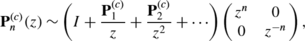  (B.4)

  where $\mathbf{P}^{(c)}_{k}$, k=1,2,… , are some constant 2×2 matrices.

This problem has the unique solution

(B.5)

The normalizing constants $h_{n}^{(c)}$ can be found as

$$ h_n^{(c)}=-2\pi i \bigl[\mathbf{P}^{(c)}_1 \bigr]_{12},\qquad \bigl(h_{n-1}^{(c)} \bigr)^{-1}=-\frac{ [\mathbf{P}^{(c)}_1 ]_{21}}{2\pi i}. $$

(B.6)

We can make a series of transformations to $\mathbf{P}_{n}^{(c)}$ to arrive at a small norm problem. Define $\mathbf{T}_{n}^{(c)}$ from the equation

$$ \mathbf{P}^{(c)}_n(z)=e^{\frac{nl}{2}\sigma_3}\mathbf{T}^{(c)}_n(z)e^{n(g(z)-\frac{l}{2})\sigma_3}, $$

(B.7)

and $\mathbf{S}_{n}^{(c)}$ as

(B.8)

Then the matrix $\mathbf{X}_{n}^{(c)}$ can be defined as

(B.9)

The jump matrices for $\mathbf{X}_{n}^{(c)}(z)$ are exponentially close to those for X _n (z), and therefore, by (4.85) and (4.86), $\mathbf{X}_{n}^{(c)}(z)$ and X _n (z) are exponentially close to each other. We are interested in the off diagonal terms of the matrix $\mathbf{X}_{1}^{(c)}$, where

$$ \mathbf{X}_n^{(c)}(z)=I+\frac{\mathbf{X}_1^{(c)}}{z}+O \bigl(z^{-2}\bigr). $$

(B.10)

One can easily see that

$$ \begin{aligned}[c] \bigl[\mathbf{X}_1^{(c)} \bigr]_{12}&= \bigl[\mathbf{P}_1^{(c)} \bigr]_{12}e^{-nl}-[\mathbf{M}_1]_{12} =-\frac{h_n^{(c)}}{2\pi i} \bigl(\pi^2 a e\bigr)^n - \frac{i}{\pi\sqrt{a}}, \\ \bigl[\mathbf{X}_1^{(c)} \bigr]_{21}&= \bigl[\mathbf{P}_1^{(c)} \bigr]_{21}e^{nl}-[ \mathbf{M}_1]_{21} =-\frac{2\pi i}{h_{n-1}^{(c)}(\pi^2 a e)^n}+\frac{i}{\pi\sqrt {a}}. \end{aligned} $$

(B.11)

The constants $h_{n}^{c}$ and $h_{n-1}^{(c)}$ are known exactly:

$$ h_{n}^{(c)}=\frac{n! \sqrt{2\pi}}{(\sqrt{na} \pi)^{2n+1}}, \qquad h_{n-1}^{(c)}=\frac{(n-1)! \sqrt{2\pi}}{(\sqrt{na} \pi)^{2n-1}}. $$

(B.12)

It follows that

$$ \begin{aligned}[c] & \bigl[\mathbf{X}_1^{(c)} \bigr]_{12}=- \frac{i}{\pi\sqrt{a}} \biggl(1- \biggl(\frac{e}{n} \biggr)^n \frac{n!}{\sqrt{2\pi n}} \biggr), \\ &\bigl[\mathbf{X}_1^{(c)} \bigr]_{21}=\frac{i}{\pi\sqrt{a}} \biggl(1- \biggl(\frac {n}{e} \biggr)^n\frac{\sqrt{2\pi}}{\sqrt{n} (n-1)!} \biggr). \end{aligned} $$

(B.13)

Applying Stirlings formula, we find that

$$ \begin{aligned}[c] \bigl[\mathbf{X}_1^{(c)} \bigr]_{12}=\frac{i}{\pi\sqrt{a}} \biggl(\frac {1}{12n}+ \frac{1}{288n^2} -\frac{139}{51840 n^3} +O\bigl(n^{-4}\bigr) \biggr), \\ \bigl[\mathbf{X}_1^{(c)} \bigr]_{21}= \frac{i}{\pi\sqrt{a}} \biggl(\frac {1}{12n}-\frac{1}{288n^2} - \frac{139}{51840 n^3} +O\bigl(n^{-4}\bigr) \biggr) . \end{aligned} $$

(B.14)

Let us now return to the discrete system of orthogonal polynomials. The normalizing constants are given as

$$ \begin{aligned}[c] h_{n,n}&=\frac{2}{\sqrt{a}} \biggl( \frac{1}{\pi^2 a e} \biggr)^n \bigl(1-[\mathbf{X}_1]_{12} \pi \sqrt{a} i \bigr) , \\ h_{n,n-1}^{-1}&=\frac{1}{2\sqrt{a}\pi^2} \bigl({\pi^2 a e} \bigr)^n \bigl(1+[\mathbf{X}_1]_{21}\pi \sqrt{a} i \bigr). \end{aligned} $$

(B.15)

Since X _n and $\mathbf{X}_{n}^{(c)}$ are exponentially close to each other, we may use the above expansion for X ₁, obtaining

$$ \begin{aligned}[c] h_{n,n}&=\frac{2}{\sqrt{a}} \biggl( \frac{1}{\pi^2 a e} \biggr)^n \biggl(1+\frac{1}{12n}+ \frac{1}{288n^2} -\frac{139}{51840 n^3} +O\bigl(n^{-4}\bigr) \biggr), \\ h_{n,n-1}^{-1}&=\frac{1}{2\sqrt{a}\pi^2} \bigl({\pi^2 a e} \bigr)^n \biggl(1-\frac{1}{12n}+\frac{1}{288n^2} + \frac{139}{51840 n^3} +O\bigl(n^{-4}\bigr) \biggr). \end{aligned} $$

(B.16)

Let us also note that in this asymptotic regime, by a similar argument, we find that the recurrence coefficients $A_{n,k}^{(\alpha )}(a)$ are exponentially close to zero, as they vanish for Hermite polynomials.

Appendix C: Deformation Equations for Orthogonal Polynomials

In this appendix, we prove the deformation equations (1.36) and (2.2). These equations are in fact quite general, and we present the proof for a general class of orthogonal polynomials. Let $\{p_{k}(x)\}_{k=0}^{\infty}$ be a system of monic polynomials satisfying the orthogonality condition

$$ \int_\mathbb {R}p_k(x)p_j(x)e^{-ax^2} \,d\mu(x)=h_k \delta _{jk}, $$

(C.1)

where dμ(x) is any measure on ℝ such that the system of orthogonal polynomials exists. We consider deformations of this system with respect to the parameter a. Let us write the three term recurrence equation, explicitly noting the dependence of each recurrence coefficient on the parameter a:

$$ xp_k(x)=p_{k+1}(x)+A_k(a)p_k(x)+B_k(a)p_{k-1}(x), \quad B_k(a)=\frac {h_k(a)}{h_{k-1}(a)}. $$

(C.2)

Notice that, since the polynomials p _k are monic, $\frac{\partial }{\partial a} p_{k}(x)$ is a polynomial of degree strictly less than k, and thus its integral against $p_{k}(x) e^{-ax^{2}}\, d\mu(x)$ is zero. Thus if we differentiate (C.1) with respect to a in the case j=k, apply the three term recurrence twice and integrate, we obtain

$$ h_k'(a)=-h_k (B_{k+1}+A_{k}+B_k ), $$

(C.3)

or equivalently

$$ \frac{\partial }{\partial a} \log h_k = -A_k- \frac{h_{k+1}}{h_k}- \frac {h_{k}}{h_{k-1}}, $$

(C.4)

where we have suppressed the notation which explicitly indicates dependence on a.

Let us use c _k,j to denote the coefficient of the x ^j term in the polynomial p _k (x), so that

$$ p_k(x)=x^k+c_{k,k-1} x^{n-1} +c_{k,k-2} x^{n-2}+ \cdots. $$

(C.5)

These coefficients depend on the parameter a, and by matching the coefficients of the x ^k term in (C.2), we see that

$$ A_k(a)=c_{k,k-1}-c_{k+1,k}. $$

(C.6)

To arrive at a deformation equation for A _k consider (C.1) with j=k−1. Differentiating with respect to a and disregarding the term for which the integral vanishes gives

$$ \int_\mathbb {R}\biggl[\frac{\partial }{\partial a} \bigl(p_k(x) \bigr) p_{k-1}(x) -x^2 p_{k-1}(x)p_k(x) \biggr]e^{-ax^2} \,d\mu(x)=0. $$

(C.7)

Applying the three term recursion twice and integrating, we obtain

$$ \biggl(\frac{\partial }{\partial a} c_{k,k-1} \biggr) h_{k-1}=A_kh_k+A_{k-1}B_k h_{k-1}. $$

(C.8)

Combining (C.6) with (C.8) both as it is written and with k↦k+1, we find

$$ A_k'(a)=B_k (A_k+A_{k-1} ) - B_{k+1} (A_{k+1}+A_{k}). $$

(C.9)

We now use (C.3) and (C.9) to differentiate (C.4) once more, obtaining

$$ \frac{\partial ^2}{\partial {a}^2} \log h_k=I_{k+1}-I_k, $$

(C.10)

where

$$ I_k=B_k \bigl(B_{k+1}+B_{k-1}+ (A_{k-1}+A_k )^2 \bigr). $$

(C.11)

It follows that the sum

$$ \sum_{k=0}^{n-1} \frac{\partial ^2}{\partial {a}^2} \log h_k $$

(C.12)

telescopes and its value is I _n −I ₀. But I ₀=0, and thus the sum (C.12) is simply I _n . After a change of variable, this proves (1.36).

We now prove (2.2). In the case that the measure of orthogonality is even, the recurrence coefficients A _k vanish, and we have

$$ I_k=B_kB_{k+1}+B_kB_{k-1} $$

(C.13)

and

$$ \begin{aligned}[c] &\sum_{k=0}^{N-1} \frac{\partial ^2}{\partial {a}^2} \log h_{2k}=\sum_{k=0}^{N-1} B_{2k+1}B_{2k+2}-B_{2k}B_{2k-1}; \\ &\sum _{k=0}^{n-1} \frac{\partial ^2}{\partial {a}^2} \log h_{2k+1}=\sum_{k=0}^{n-1} B_{2k+2}B_{2k+3}-B_{2k}B_{2k+1} \end{aligned} $$

(C.14)

which are again telescoping sums, and we obtain (2.2) after a change of variables.

References

Baik, J., Deift, P., Johansson, K.: On the distribution of the length of the longest increasing subsequence of random permutations. J. Am. Math. Soc. 12(4), 1119–1178 (1999)
Baik, J., Jenkins, R.: Limiting distribution of maximal crossing and nesting of Poissonized random matchings, preprint. arxiv.org/abs/1111.0269
Baik, J., Kriecherbauer, T., McLaughlin, K.T.-R., Miller, P.D.: Discrete Orthogonal Polynomials. Asymptotics and Applications. Ann. Math. Studies, vol. 164. Princeton University Press, Princeton and Oxford (2007)
Baik, J., Rains, E.M.: Symmetrized random permutations. In: Bleher, P.M., Its, A.R. (eds.) Random Matrix Models and Their Applications. MSRI Publications, vol. 40. Cambridge University Press, Cambridge (2001)
Bleher, P.M., Its, A.: Double scaling limit in the random matrix model: the Riemann-Hilbert approach. Commun. Pure Appl. Math. 56(4), 433–516 (2003)
Bleher, P.M., Its, A.: Asymptotics of the partition function of a random matrix model. Ann. Inst. Fourier 55(6), 1943–2000 (2005)
Bleher, P.M., Liechty, K.: Uniform asymptotics for discrete orthogonal polynomials with respect to varying exponential weights on a regular infinite lattice. Int. Math. Res. Not. rnq081v2–rnq081 (2010)
Chester, C., Friedman, B., Ursell, F.: An extension of the method of steepest descents. Proc. Camb. Philos. Soc. 53(3), 599–661 (1957)
Claeys, T., Kuijlaars, A.: Universality in the double scaling limit in random matrix models. Commun. Pure Appl. Math. 59(11), 1573–1603 (2006)
Corwin, I., Hammond, A.: Brownian Gibbs property for Airy line ensembles, preprint. arXiv:1108.2291
Corwin, I., Quastel, J., Remenik, D.: Continuum statistics of the Airy2 process, preprint. arxiv.org/abs/1106.2717
Crescimanno, M., Naculich, S.G., Schnitzer, H.J.: Evaluation of the free energy of two-dimensional Yang-Mills theory. Phys. Rev. D 54, 1733–1746 (1996)
Deift, P.: Orthogonal Polynomials and Random Matrices: A Riemann-Hilbert Approach. Courant Lecture Notes in Mathematics, vol. 3 (1999)
Deift, P., Its, A., Krasovsky, I.: Asymptotics of the Airy-kernel determinant. Commun. Math. Phys. 278(3), 643–678 (2008)
Deift, P., Li, L.C., Tomei, C.: Toda flows with infinitely many variables. J. Funct. Anal. 64, 358–402 (1985)
Deift, P., Kriecherbauer, T., McLaughlin, K.T.-R., Venakides, S., Zhou, X.: Uniform asymptotics for polynomials orthogonal with respect to varying exponential weights and applications to universality questions in random matrix theory. Commun. Pure Appl. Math. 52, 1335–1425 (1999)
Deift, P., Nanda, T., Tomei, C.: Ordinary differential equations and the symmetric eigenvalue problem. SIAM J. Numer. Anal. 20(1), 1–22 (1983)
Deift, P., Zhou, X.: A steepest descent method for oscillatory Riemann-Hilbert problems. Asymptotics for the MKdV equation. Ann. Math. 137, 295–368 (1993)
Deift, P., Zhou, X.: Asymptotics for the Painlevé II equation. Commun. Pure Appl. Math. 48(3), 277–337 (1995)
Douglas, M.R., Kazakov, V.A.: Large N phase transition in continuum QCD2. Phys. Lett. B 319, 219–230 (1993)
Eynard, B.: A concise expression for the ODE’s of orthogonal polynomials, preprint. arXiv:math-ph/0109018
Feierl, T.: The height of watermelons with a wall. J. Phys. A 45, 095003 (2012)
Fokas, A., Its, A., Kapaev, A., Novokshenov, V.: Painlevé Transcendents: The Riemann-Hilbert Approach. AMS Surveys and Monographs, vol. 128 (2006)
Forrester, P.J.: Log-Gases and Random Matrices. Princeton University Press, Princeton (2010)
Forrester, P.J., Majumdar, S.N., Schehr, G.: Non-intersecting Brownian walkers and Yang-Mills theory on the sphere. Nucl. Phys. B 844(3), 500–526 (2011)
Gillet, K.: Asymptotic behaviour of watermelons, preprint. arxiv.org/abs/math/0307204
Hastings, S.P., McLeod, J.B.: A boundary value problem associated with the second Painlevé transcendent and the Korteweg-de Vries equation. Arch. Ration. Mech. Anal. 73, 31–51 (1980)
Its, A., Krasovsky, I.: Hankel determinant and orthogonal polynomials for the Gaussian weight with a jump. In: Baik, J., Kriecherbauer, T., Li, L.C., McLaughlin, K.T.-R., Tomei, C. (eds.) Integrable Systems and Random Matrices. Contemp. Math., vol. 458. Am. Math. Soc., Providence (2008)
Johansson, K.: Discrete polynuclear growth and determinantal processes. Commun. Math. Phys. 242, 277–329 (2003)
Karlin, S., McGregor, J.: Coincidence probabilities. Pac. J. Math. 9, 1141–1164 (1959)
Katori, M., Tanemura, H.: Symmetry of matrix-valued stochastic processes and noncolliding diffusion particle systems. J. Math. Phys. 45, 3058–3085 (2004)
Katori, M., Tanemura, H., Nagao, T., Komatsuda, N.: Vicious walk with a wall, noncolliding meanders, and chiral and Bogoliubuv-de Gennes random matrices. Phys. Rev. E 68, 021112 (2003)
Krasovsky, I.V.: Correlations of the characteristic polynomials in the Gaussian unitary ensemble or a singular Hankel determinant. Duke Math. J. 139(3), 581–619 (2007)
Kobayashi, N., Izumi, M., Katori, M.: Maximum distributions of noncolliding Brownian paths. Phys. Rev. E 78, 051102 (2008)
Moreno-Flores, G., Quastel, J., Remenik, D.: Endpoint distribution of directed polymers in 1+1 dimensions, preprint. arxiv.org/abs/1106.2716
Prähofer, M., Spohn, H.: Scale invariance of the PNG droplet and the Airy process. J. Stat. Phys. 108(5–6) 1071–1106 (2002)
Rambeau, J., Schehr, G.: Distribution of the time at which N vicious walkers reach their maximal height. Phys. Rev. E 83, 061146 (2011)
Schehr, G.: Extremes of N vicious walkers for large N: application to the directed polymer and KPZ interfaces, preprint. arXiv:1203.1658
Schehr, G., Majumdar, S.N., Comtet, A., Randon-Furling, J.: Exact distribution of the maximal height of p vicious walkers. Phys. Rev. Lett. 101, 150601 (2008)
Szegö, G.: Orthogonal Polynomials, 4th edn. Colloquium Publications, vol. 23. Am. Math. Soc., Providence (1975)
Tracy, C., Widom, H.: Level-spacing distribution and the Airy kernel. Phys. Lett. B 305, 115–118 (1993)
Tracy, C., Widom, H.: Level-spacing distribution and the Airy kernel. Commun. Math. Phys. 159, 151–174 (1994)
Tracy, C., Widom, H.: On orthogonal and symplectic matrix ensembles. Commun. Math. Phys. 177, 727–754 (1996)
Tracy, C., Widom, H.: Nonintersecting Brownian excursions. Ann. Appl. Probab. 17(3), 953–979 (2007)
Acknowledgements
I would like to thank Grégory Schehr and Peter Forrester for bringing this problem to my attention, and Schehr for useful correspondence. I would also like to thank Jinho Baik and Peter Miller for discussions, advice, and feedback.
Author information
Authors and Affiliations
Corresponding author