
Abstract
Defining general criteria for the acceptability of defects within industrial components is often complicated, since the specific load conditions and the criticality of the given application should be considered individually. In order to minimize the risk of failure, high safety factors are commonly adopted during quality control. However this practice is likely to cause the rejection of components whose defects would be instead acceptable if a more sound knowledge of the component behaviour were achieved. Parts produced by additive manufacturing (AM) may suffer from various defects, including micro- or macro-holes, delamination and microstructural discontinuities. Such processes, which are specially suitable for one-off components, require robust and reliable inspection before a part is accepted or rejected, since the refusal of even a single part at the end of the production process represents a significant loss. For this reason, it would be very useful to simulate in a reliable way whether a certain defect is truly detrimental to the proper working of the part during operation or whether the component can still be used, despite the presence of a defect. To this purpose, the paper highlights the benefits of a synergistic interaction between Industrial X-ray computed tomography (XCT) and finite element analysis (FEA). Internal defects of additively manufactured parts can be identified in a non-destructive way by means of XCT. Then FEA can be performed on the XCT-based virtual model of the real component, rather than on the ideal CAD geometry. A proof of concept of this approach is proposed here for a reference construct produced in an Aluminium alloy by AM. Numerical results of the proposed combined XCT–FEA procedure are contrasted with experimental data from tensile tests. The findings sustain the reliability of the method and allow to assess its full provisional accuracy for parts of cylindrical geometry designed to operate in the elastic field. The paper moves a step beyond the present application limits of tomography as it is currently employed for AM parts and it evidences instead the possibility of extending the usage of tomography to acceptance testing and prediction of operative behaviour.
1 Introduction
In the past, components made by the layer-by-layer addition of material were mainly considered as visualization tools or used for assembly testing. To the contrary, nowadays AM techniques are establishing themselves as effective methods to produce final parts, including metal ones. Over the last decade, rapid tooling, i.e. the fabrication of moulds and dies, and digital manufacturing, i.e. the direct fabrication of end-usable products or parts from additive machines, have been studied extensively by several researchers. The continuous progress in the field of materials science has made it possible to introduce new metal powders on the market that are adequate for metal end-products, with applications in the aerospace, dental and medical sectors [1, 2].
The main benefit of AM technology is that it enables the flexible production of customized products without introducing any cost penalties during manufacturing. Product customization can lead to an increase in the customers’ perceived product value and, thus, to a greater willingness to pay. This is why firms can charge a price premium [3]. Therefore, a finished AM part has a high perceived value (it is often a one-of-a-kind part), and a rejected part at the end of production represents a significant loss. Since AM parts may suffer from various defects, such as micro- or macro-holes, delamination and discontinuities due to the balling effect, it is important to understand whether a microstructural fault can truly hinder the function of the part during operation or whether it is possible to tolerate the presence of a the defect.
An increasing number of contributions in the literature report that defects of AM parts can be identified in a non-destructive way by means of X-ray computed tomography or XCT [4, 5]. One of the significant advantages of XCT over other non-contact or contact measurement systems is that areal surface parameters as defined in ISO 25178-2: 2012 can be extracted from the internal surfaces of AM components [6]. XCT is currently considered the best experimental approach to investigate the internal features of parts, as for example pores, their morphology and distribution [7, 8]. On the contrary, tomography has not been firmly established as a measurement tool yet, unlike other dimensional metrology methods. Industrial tomography image noise and spatial image resolution have significant effects on the accuracy of measurements. However, some authors have pointed out that the industrial XCT definition is accurate enough to obtain a mathematical model of porous materials that is suitable for predictive behaviour analysis [9].
The present paper moves a first step beyond the current application limits of tomography in AM parts [6], and evidences the possibility of extending tomography to new potential applications, including acceptance testing, verification of expected operative behaviour and assessment of defect acceptability. In fact, the numerical models reconstructed by means of XCT are used as a basis to develop FE simulations that, in this way, are able to account for real microstructural details and defects. In order to validate the model, experimental tests are performed on AlSi10Mg AM parts.
The number of different Al alloys that are available for AM is still rather limited. One reason for this is that Al alloys, unlike Ti alloys, are comparatively easy to machine, and therefore the costs of Al machined parts are comparatively low and the production of Al parts by AM not often economically competitive [10]. Currently, the most common aluminium alloy for AM is AlSi10Mg, which is used to produce strong and high dynamic load-bearing components. As a consequence, AlSi10Mg parts are optimal for use in such areas as aerospace engineering and automotive industry [11].
This paper evidences that, by combining tomography and FEA, it is possible to predict the real behaviour of AM AlSi10Mg parts affected by manufacturing defects, straightforwardly if the part is designed to operate in the elastic range. A proof of concept is given, currently limited to simple geometries. In order to assess the accuracy of the model to simulate the behavior of AM parts with internal discontinuities, two different holes were arbitrarily introduced in cylindrical specimens, namely: a lenticular biconvex shape hole and a spherical one. Relatively simple defect geometries have been chosen in order to assess a first feasibility of the proposed approach. The designed defects were investigated by means of XCT before mechanical testing of the specimens. The possible discrepancies between the designed defects and manufactured defects were collected. XCT data were used to obtain a mathematical model of the as-manufactured part, including defects. The obtained model was then used to predict the behaviour of the defected part when it is subjected to a working load. Finally, the real and simulated performance were compared.
2 Methods
The present paper aims at an initial investigation of a combined XCT–FEA approach to support the decision about the acceptability of an AM part with inner defects. The proposed procedure consists of:
-
XCT scanning of parts built by AM;
-
reconstruction of the numerical model of the as-manufactured part with its possible defects;
-
running of a FE simulation in order to determine the stress values in the as-manufactured part;
-
decision on the acceptability of the part, by taking into account possible stress intensification in the proximity of defects.
In order to attain a proof of concept of the method, the following steps were followed.
-
1.
AlSi10Mg (Table 1) simple cylindrical specimens were manufactured with and without designed defects (Table 2) by EOSINT M 270 (Fig. 1).The specimens were built with the main axis parallel to the growth direction Z. The geometry of the specimens and the shape of the designed defects are relatively simple, as compared to usually more complex ones in the field of AM. This approach was chosen in order to setup the method and to attain a first proof of concept, to be further validated by using more complex shapes.
Table 1 Weight percentage composition of AlSi10Mg Table 2 Used specimens Fig. 1 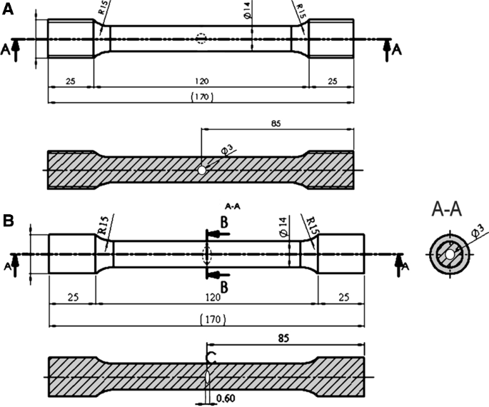
Specimens with designed defects: a spherical defect; b lenticular biconvex defect
-
2.
The specimens were scanned by means of a North Star Imaging X-View CT X5000.

X5000-CT is a seven-axis universal X-ray imaging system that was designed for the inspection of large objects by means of a digital detectors array (DDA). The instrument has the following characteristics [12]:
-
Voltage range 10 kV ÷ 450 kV;
-
Minimum focal spot size < 5 µm;
-
Maximum resolution = 5 µm.
The resolution to be used in the scan was chosen after a preliminary test. A high resolution implies very long acquisition time. In terms of results, the effect of different resolution levels is shown in Fig. 2: a low resolution acquisition (63.5 µm) returns a greater and more blurred defect model than that returned by high resolution (19 µm).

Resolution effect on the detection of defects: a low resolution, i.e. great voxel side; b high resolution, i.e. small voxel size
In order to be attractive for everyday industrial production, the XCT–FEA procedure must be: (i) fast, that is to say requiring the minimum time, and consequently the minimum cost; and (ii) conservative, in the sense that it should avoid the risk of underestimating defects and stress levels. On the contrary, the procedure should guarantee that stress in the proximity of a defect is predicted with a sufficient excess safety margin with respect to what will happen in the worst case in real working conditions. The low resolution acquisition satisfies both requirements, since it requires short measurement times and it also overestimates the real defect size, due to the indeterminacy of the edges.
It was also important to choose an appropriate frame capture rate (FPS frames per second), as this affects the saturation of the detector, i.e. the maximum signal that this can detect without losing information. If too low, the FPS value leads to a low image contrast; if too high, the FPS value causes detector over-saturation, which results in a loss of out-of-signal information at each single voxel. Once the scanning conditions had been established, a calibration scan was performed before the samples were scanned.
The specimens were scanned according to the following parameters:
-
Voltage = 230 kV;
-
Current = 490 μA;
-
Frames per second = 2.6;
-
Specimens orientation = Z = vertical axis;
-
Scanning time = 32 min;
-
Pixel pitch = 0.063 mm.
In accordance with literature data [13], the X-ray beam was filtered during the scanning process using a Cu filter (0.3 mm thick) in order to reduce beam-hardening effects. This filter cuts off the low frequency radiation that is captured by the specimen and which is a source of noise. A Pb filter (0.1 mm thick) was also used for the detector in order to reduce signal scattering.
-
3.
Tomographic data were used to build a FE model, by importing the scan results in the STL file format into ANSYS Workbench. The model was meshed by dedicated tools. In particular, the mesh refining algorithms at the defect area and the connection of the locally refined mesh to the general one required a thorough analysis (Fig. 3b).
Fig. 3 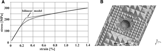
a Experimental stress–strain curve of a specimen without defect and bilinear elastic–plastic model used for the simulations; b mesh refining at a defect zone and connection of the locally refined mesh to the general one
-
4.
Tensile tests were performed in accordance with UNI EN ISO 6892-1:2009. The tensile tests on the specimens without defects allowed to measure the mechanical response of the material. Strain gauges with 0.3 mm grit were mounted onto all the specimens before tensile testing. Two different positions were chosen for each sample: one at the same axial position of the defect, and the other along the specimen axis 40 mm far from the defect, still within the reduced section. Three strain gauges were placed at 120° from each other for each position (Fig. 4). The data from the strain gauges were collected by a 128-channel Vishay System 7000-128-SM. The strain gauge readings and the applied forces were collected for each sample during the tensile test. The strain gauges allowed the maximum strain value and its position to be evaluated. The sampling rate of the data from the strain gauges and that of the testing machine were the same.
Fig. 4 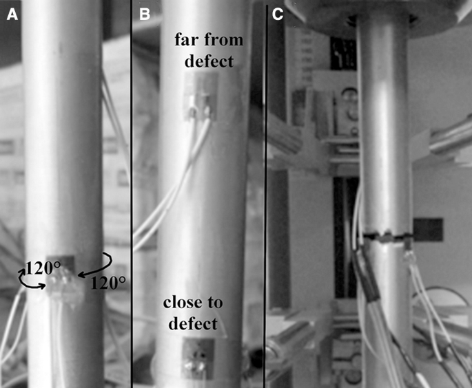
Two different positions on each sample were chosen for mounting the strain gauges: one close to the axial position of the defect and the other 40 mm far from it. Three extensometers were mounted at 120° from each other for each position
-
5.
In the FE environment, a bilinear elastic–plastic material model was chosen to describe the behaviour of the specimens under tensile loading. The equations of the elastic and of the plastic tracts were calculated by matching the experimental stress–strain curves of the specimens without designed defects. The bilinear model can then be used to describe the material within the FE environment and to perform simulations of any other complex geometry. In this paper, after fixing the boundary conditions the simulation was performed and the results were compared with the experimental data obtained for the specimens with defects by using 2000 measured points for each specimen. At each point, the experimental strain value was compared to that predicted by the simulation.


The same procedure was repeated for all the specimens.
3 Results and discussion
A bilinear elastic–plastic model was computed from the experimental stress–strain curves of the specimens without designed defects, as shown in Fig. 3a, and used to describe the response of the material in the following simulations. The adoption of a bilinear elastic–plastic model entails a critical response as a result of the slope variation occurring at the theoretical intersection between the two linear tracts (Fig. 3a). It is possible to assume that probable weaknesses in the simulations will emerge in this area: the bilinear model has in fact different derivatives when the junction is approached from the right or from the left, whereas the experimental curve of the real material has a continuous derivative. In other words, this is an intrinsic limitation that unavoidably originates from the adopted material response model, and therefore its effects will be disregarded when discussing the results of the scanning and modelling procedure. On the other hand, the choice of more complex models is not practically feasible, since it would result in a greater time and computational source consumption.
Figures 5 and 6 show the tensile test results: the values refer to 5 samples for each kind of specimens. The dotted lines in Fig. 5 represent the tensile and yield strength values (Fig. 5), that are reported in the material technical specification. The tensile strength of the samples without designed defects is lower than the nominal tensile strength of the material, while the yield limit is greater than the nominal value stated by the producer [14]. The introduction of a designed defect results in insignificant variations in the yield strength, while variations in the tensile strength are significant and dependent on the shape of the defects. It is worth noting that the introduced defects have different geometries in 3D, but their projections onto the specimen growth plane have the same geometry and the same area.

Mechanical performances of the specimens with and without designed defects: a yield strength; b tensile strength. Dotted lines represent the tensile and yield strength values that are reported in the material datasheet [14]

a Elongation of the specimens with and without designed defects. b Rupture surface of a specimen with designed spherical defect
The experimentally determined elongation at break (Fig. 6a) is 50% lower than that reported in the material datasheet [14]. Elongation at break varies in the presence of defects in the same way as tensile strength does. The introduction of a defect into the specimens under investigation results in a significant loss in elongation that depends on the shape of the defect, even for equal reduction of the effective load-bearing cross-sectional area. Figure 6b shows the rupture surface of a specimen with a designed spherical defect.
Figures 7 and 8 show, for the specimens with designed defects, the predicted strain values obtained by FEA (by applying the material response model shown in Fig. 3a) and compare them to the average value of the measured strains. The average value refers to the medium value of the three strain gauges placed on the same circumference: close to and far from the defects, as shown in Figs. 7 and 8 respectively. In the graphs in Figs. 7 and 8 the bisector is shown as a black solid line and referred to as the trend of “perfect correspondence” between the modeled values and the experimental ones. In all cases, and in both zones, the simulated strain and the measured one are in very good agreement for strain values lower than 0.2%, that is to say in the elastic region. In the 0.2–0.5% measured strain range, the curves show a flex in which they deviate to a shifted linear trend. For values greater than 0.5%, there is a constant shift between the modeled data and the experimental ones. The adoption of the bilinear response model for the material probably generates a deviation at the point of transition between the elastic field and the plastic field. A more sophisticated material model would likely overcome this critical aspect. It is also important to consider that the FE model does not describe the rupture of the specimens. For the area close to the lenticular biconvex defects, the discrepancy between the predicted values and the measured ones tends to increase when the strain increases. In the case of the area close to the spherical defect, and for both graphs showing the results far from the defect zone, the shift between the modelled values and the measured ones tends to be constant when the strain increases. Above 0.5%, the predicted strain and the measured one are de facto linearly correlated, even though there is an offset value. The method is fully reliable for the considered cylindrical geometry in the elastic range, which most industrial components are designed to operate in. Provisional accuracy after the yield point would be possible by an appropriate tuning between the numerical and the experimental results.

Predicted strain obtained by FEA versus the average value of the measured strains in the area close to the defect zone: a spherical defect; b lenticular biconvex defect

Predicted strain obtained by FEA versus the average value of the measured strains in the area far from the defect zone: a spherical defect; b lenticular biconvex defect
Even if there is a rapidly increasing number of studies in the literature aimed at understanding the nature and the source of defects in AM processes [15], in situ monitoring and control solutions make it possible to detect the formation of defects in real time, but they are unable to prevent it. Though instant feed-back mechanisms are implemented, the risk that a defect may develop just before the end of the job causes a serious economic damage. However, not all defects are prejudicial to usage. As a consequence, the prompt detection of the presence of defects and the reliable prediction of their criticality may serve to discriminate if the finished part should be rejected or not. The integrated XCT–FEA-based approach proposed here may effectively serve to the purpose.
Typical lab-based XCT can take up to 30 min to produce a 3D model of an object [16]. From this point of view, checking an AM part by XCT causes an increase in cost and production time, but the efficiency loss associated to this inspection operation may turn to be preferable both to the risk of a rupture in service or to the rejection of defected but still usable part.
4 Conclusion
AlSi10Mg tensile test specimens were manufactured, with and without designed defects, by means of the additive manufacturing technique. Two different types of defects were deliberately introduced during manufacturing, namely: a lenticular biconvex defect and a spherical one. The real numerical model of the samples, including defects, was constructed by means of industrial tomography. The model was used as a basis for FE simulations to predict the behaviour of a component under tensile loading. The use of XCT models having a lower resolution than that needed for the exact definition of internal defects leads to overestimate the stress intensification and gives therefore a higher safety margin. The FEA results were compared to those obtained from a mechanical test. In more detail, the analysis was focused on a first area in close proximity to the defect and on a second area far from the defect. For the considered geometry, the mechanical properties simulated by means of the FEA correlate well with the average of the values experimentally measured in the elastic field. A shift is observed between the modeled data and the experimental ones in the plastic field, but the XCT-based FEA maintains its provisional efficacy. As a conclusion, a proof of concept is provided that an approach based on XCT and FEA could be promising for the acceptance/rejection step of additive manufactured metal parts.
References
Atzeni, E., Salmi, A.: Economics of additive manufacturing for end-usable, metal parts. Int. J. Adv. Manuf. Technol. 62, 1147–1155 (2012)
Mengucci, P., Gatto, A., Bassoli, E., Denti, L., Fiori, F., Girardin, E., Barucca, G.: Effects of build orientation and element partitioning on microstructure and mechanical properties of biomedical Ti-6Al-4 V alloy produced by laser sintering. J. Mech. Behav. Biomed. 71, 1–9 (2017)
Weller, C., Kleer, R., Piller, F.T.: Economic implications of 3D printing: market structure models in light of additive manufacturing revisited Int. J. Prod. Econ. 164, 43–56 (2015)
Xu, Z., Hyde, C.J., Thompson, A., Leach, R.K., Maskery, I., Tuck, C., Clare, A.T.: Staged thermomechanical testing of nickel superalloys produced by selective laser melting. Mater. Des. 133, 520–527 (2017)
Maskery, I., Aboulkhair, N.T., Corfield, M.R., Tuck, C., Clare, A.T., Leach, R.K., Wildman, R.D., Ashcroft, I.A., Hague, R.J.M.: Quantification and characterisation of porosity in selectively laser melted Al–Si10–Mg using X-ray computed tomography. Mater. Charact. 111, 193–204 (2016)
Townsend, A., Senin, N., Blunt, L., Leach, R.K.: Taylor Surface texture metrology for metal additive manufacturing: a review. Precis. Eng. 46, 34–47 (2016)
Seifi, M., Christiansen, D., Beuth, J., Harrysson, O., Lewandowski, J.J.: Process mapping fracture and fatigue behavior of Ti-6al-4v produced by EBM additive manufacturing Ti. In: The 13th World Conference on Titanium Edited by: Adam Pilchak et al. TMS (The Minerals, Metals & Materials Society) (2015)
Thompson, A., Maskery, I., Leach, R.K.: X-ray computed tomography for additive manufacturing: a review. Meas. Sci. Technol. 27, 072001 (2016)
Kerckhofs, G., Pyka, G., Moesen, M., Van Bael, S., Schrooten, J., Wevers, M.: High-resolution microfocus X-ray computed tomography for 3D surface roughness measurements of additive. Adv. Eng. Mater. 15(3), 153–158 (2013)
Herzog, D., Seyda, V., Wycisk, E., Emmelmann, C.: Additive manufacturing of metals. Acta Mater. 117, 371–392 (2016)
SLM Solutions, 3D Metals: AlSi10Mg. https://slm-solutions.com/download-center. Accessed 1 Aug 2018
X-VIEW CT brouchure. https://4nsi.com/brochures/x5000-brochure.pdf. Accessed 1 Aug 2018
Ziółkowski, G., Chlebus, E., Szymczyk, P., Kurzac, J.: Application of X-ray Ct method for discontinuity and porosity detection in 316 l stainless steel parts produced with SLM technology. Arch. Civ. Mech. Eng. 14, 608–614 (2014)
EOS GmbH—Electro Optical Systems Material data sheet. https://www.eos.info/eos_binaries0/eos/8d75e73a9911faca/7a06cf1cc0ad/AlSi10Mg_9011-0024_M290_Material_data_sheet_12-17_en.pdf (2013). Accessed 1 Aug 2018
Grasso, M., Colosimo, B.M.: Process defects and in situ monitoring methods in metal powder bed fusion: a review. Meas. Sci. Technol. 28, 044005 (2017)
Warnett, J.M., Titarenko, V., Kiraci, E., Attridge, A., Lionheart, W.R.B., Withers, P.J., Williams, M.A.: Towards in-process X-ray CT for dimensional metrology. Meas. Sci. Technol. 27, 035401 (2016)
Acknowledgements
The research received financial support by Regione Emilia Romagna under the DL 74/2012.
Author information
Authors and Affiliations
Corresponding author
Rights and permissions
Open Access This article is distributed under the terms of the Creative Commons Attribution 4.0 International License (http://creativecommons.org/licenses/by/4.0/), which permits unrestricted use, distribution, and reproduction in any medium, provided you give appropriate credit to the original author(s) and the source, provide a link to the Creative Commons license, and indicate if changes were made.
About this article

Cite this article
Esposito, F., Gatto, A., Bassoli, E. et al. A Study on the Use of XCT and FEA to Predict the Elastic Behavior of Additively Manufactured Parts of Cylindrical Geometry. J Nondestruct Eval 37, 72 (2018). https://doi.org/10.1007/s10921-018-0525-x
Received:
Accepted:
Published:
DOI: https://doi.org/10.1007/s10921-018-0525-x