Truth Diagrams Versus Extant Notations for Propositional Logic

Abstract

Truth diagrams (TDs) are introduced as a novel graphical representation for propositional logic (PL). To demonstrate their epistemic efficacy a set of 28 concepts are proposed that any comprehensive representation for PL should encompass. TDs address all the criteria whereas seven other existing representations for PL only provide partial coverage. These existing representations are: the linear formula notation, truth tables, a PL specific interpretation of Venn Diagrams, Frege’s conceptual notation, diagrams from Wittgenstein’s Tractatus, Pierce’s alpha graphs and Gardner’s shuttle diagrams. The comparison of the representations succeeds in distinguishing ideas that are fundamental to PL from features of common PL representations that are somewhat arbitrary.

1 Introduction

Truth Diagrams have been designed as a new representational system for propositional logic (PL) (sentential calculus). Representations for PL already exist, including the linear formula notation and truth tables, which are commonly used for reasoning and taught to most students of logic. Historically, several visual notations for propositional logic have also been proposed (some are examined below), so why develop a new representation?

The study of the nature of representational systems has advanced substantially over the last three decades (e.g., Glasgow et al. 1995; Hegarty 2011; Shimojima 2015). Alternative representations for a domain can substantially determine what information is accessible, how easily inferences can be made and even what things can be discovered (Zhang 1997). Poor representations dramatically increase the effort to solve problems (e.g., Cheng 2004), potentially by more than an order of magnitude (Kotovsky et al. 1985). The representation used by a learner not only affects how learning happens and how easily it occurs, but the representation can substantially determine what concepts are acquired and the problem solving methods that are mastered (Cheng 2002, 2011). Recommendations and guidelines for the design of effective representations abound (e.g., Hegarty 2011). Thus, a more principled and systematic approach to the design of a representation for PL is now more feasible than it was in the past. TDs are the outcome of such an effort.

In the field of logic, the potential value of diagrammatic representations is well recognised. For set theory and syllogisms, Euler and Venn diagrams are well-known spatial representations (Euler 1768; Venn 1880/1971). New graphical notations have even recently been invented for syllogisms, such as Englebretsen’s (1992) linear diagrams and Cheng’s (2014) Category Pattern Diagrams, and for sets, such as Set Space Diagrams (Gottfried 2014), which were derived from Cheng’s (2011) Probability Space Diagrams. Historically, diagrammatic representations were considered only to be of heuristic value, but the landmark work of Shin (1995) showed that inference with diagrams can be as rigorous as with sentential notations. Since her work other formal diagrammatic logic representations have been developed (e.g., Howse et al. 2005), but opportunities remain for an improved representation for PL.

As the formula notation currently dominates reasoning and learning about PL, attempts have been made to supplement this sentential notation with alternative representations. For example, Hodges (2001) introduced a tableau method to promote the use of proof trees and Tarski’s World by Barker-Plummer et al. (2008) is a computer simulated blocks world that concretely instantiates formulas.

So TDs aim to provide a more effective representation for PL. The effectiveness of a representation may, in general, be evaluated in at least three ways. The first is epistemic: how completely does a representation encode the full range of concepts associated with the target domain? The second is cognitive and psychological: how well does the representation support the mental access to and the processing of information about the domain? The third is pedagogic: to what extend does a representation support learning? We focus on the first, because it is foundational: representations that do not allow one to express the full range of concepts that are important to a domain will obviously hinder our thinking and learning about the whole domain. The knowledge that a representation should be able to express, in itself, without recourse to other representations, should extend from the primitive elementary concepts to overarching explanations about the fundamental nature of the domain, and all the levels between, such as the laws and principles, key categories of objects, examples of typical and extreme cases, and accounts of how they interrelate.

So, the next (second) section lists the full range of ideas that comprises a good knowledge of PL, conceptual scope criteria, against which the coverage of PL representations may be judged. The third section examines seven existing representations for PL and shows that their coverage is limited in terms of the conceptual scope criteria. Truth Diagrams are introduced in section four and descriptions of the components of the system shows that it satisfies the full range of conceptual scope criteria. The final discussion section considers implications for our general understanding of the nature of PL made possible through the comparison of the representations.

2 Conceptual Scope Criteria

What range of ideas should one possess in order to have a good knowledge of PL? Twenty eight concepts are identified, which are loosely organized into nine thematic groups, and presented in order of increasing sophistication (with examples using the conventional formula notation).

• CS1. Basic elements of PL:

  • CS1.1. Truth values: true, T, and false, F.

  • CS1.2. Variables that stand for propositions; typically represented by letters (e.g., P, Q).

  • CS1.3. Assignment of truth values to propositional variables (e.g., P = T, Q = F).

• CS2. Relations among variables:

  • CS2.1. Expressions of relations among variables (e.g., (P & Q, Q ⇒ R)).

  • CS2.2. Syntactic rules for generating well-formed expressions, which may include legal but odd examples (e.g., ¬(¬(¬(P))), (P & P) & (P & P)).

  • CS2.3. Expressions of relations between relations, such as their equivalence or not (e.g., P ⇒ Q = ¬P v Q).

• CS3. Operators:

  • CS3.1. Operators as procedures to construct relations among variables (connectives; e.g., ¬, &, v, ⇒).

  • CS3.2. Arity of operators (e.g., unary, binary, ternary).

  • CS3.3. Nature of operators (e.g., commutative, associative).

  • CS3.4. The set of operators chosen for a PL system (e.g., (¬, ⇒) versus (¬, &, v, ⇒ ⇔)).

• CS4. Cases:

  • CS4.1. A case (interpretation, model) — a particular combination of truth values assigned to each variable in an expression (e.g., given P & Q; P = T, Q = F; or one truth table row).

  • CS4.2. Assignment of a truth value to a case or relation (e.g., P & Q = T).

  • CS4.3. Contrasting cases (e.g., given P & Q, compare (P = T, Q = F) versus (P = F, Q = T); two columns in a truth table).

• CS5. Inference:

  • CS5.1. Inference rules (e.g., natural deduction, Peirce’s rules of Alpha graphs—see below).

  • CS5.2. Proof of the validity of an inference, including the processes to manage inferences and proofs (e.g., recording the discharge of assumptions).

  • CS5.3. Determining the validity of an inference independently of executing a proof (e.g., truth table test).

  • CS5.4. Overall status of a relation or an inference in terms of its cases (e.g., tautology—all cases are T; satisfiable—at least one case is T; contradiction, all cases are F).

• CS6. Acceptability of the inference system:

  • CS6.1. Meta-variables, so we can conveniently consider whole formulas (e.g., A = P & Q, B = P v Q, A ⇒ B).

  • CS6.2. Soundness (i.e., all inferences from core rules are valid).

  • CS6.3. Completeness (i.e., all tautological formulas can be proved).

• CS7. Justification of the inference rules:

  • CS7.1. Explanation of why the structure of core inference rules yield valid results (e.g., why is v-elimination more complex than &-elimination?).

  • CS7.2. Explanation of why other seemingly plausible rules are not valid (e.g., PvQ ⊢ P is not valid).

  • CS7.3. Explanation of why certain counter-intuitive inferences are valid (e.g., P, ¬P ⊢P; why can anything be inferred from a contradiction?).

• CS8. Overarching concepts: this group includes general notions that underpin the nature of PL, some of which are often not addressed explicitly.

  • CS8.1. The implication operator (⇒), the conditional proof rule and valid inferences (⊢), are closely related. What is the nature of this relation?

  • CS8.2. Unary and binary operators dominate PL; why are ternary and greater arity operators hardly considered in typical texts (see below)?

  • CS8.3. At an elementary level, truth and falsehood are essentially symmetric in PL, but is the emphasis of truth in treatments of PL essentially arbitrary or is it fundamental?

  • CS8.4. Valid inference is prized in logical thinking, but what is the nature of invalid inference and how are the two related?

• CS9. Alternative representations:

  • CS9. How well does a representation aid the comprehension of other representations? For example, does it provide insight into why inference rules are valid in other representations?

The 28 concepts show the richness of ideas that PL encompasses. The reader may wish to add further concepts or treat some as less important, but, as we will see, this list is sufficient to show the widely varying epistemic efficacies of our target representations.

3 Conceptual Scope of Existing PL Representations

Seven representations are presented in three groups: (1) the main notations for PL; (2) early visualizations of PL, without accompanying inference rules; (3) diagrammatic reasoning systems for PL. The grouping, and order of representations within groups, is primarily for the sake of exposition. (The analysis of the systems does not depend on this informal classification nor are any claims made about historical precedence in relation to their coverage of the conceptual scope criteria.)

3.1 Current Notations

The linear formula notation and truth tables are the chief representations for working with and teaching PL. Here, these texts have been selected as a representative sample of the use of these representations: Suppes (1957), Carnap (1958) Lemmon (1965), Brody (1973), Hodges (2001), Barker-Plummer et al. (2008), Barwise et al. (2011). Claims below about the general way in which the formula notation and truth tables are used is in relation to this set of texts.

3.1.1 Formula Notation

The formula notation satisfies many of the conceptual scope criteria but fairs poorly on the later categories. The formula notation represents truth values by capital letters (conceptual criteria CS1.1), propositions are represented by italic letters (CS1.2) and “equations” can be used to assign truth values to variables (e.g., Lemmon 1965). (See previous section for examples in the formula notation.) Operators are represented by symbols whose form are established by convention, and the shapes of (non)commutative operators are often (a)symmetrical, but otherwise are largely arbitrary (CS3.1). The operators are binary connectives (CS2.1) and are applied to formulas to express complex relations including odd examples (see CS2.2, above). Equations can be used to assign a truth values to a formula (CS4.3). Similarly, a truth value may be assigned to a case represented by a collection of equations in parentheses that assigns truth values to variables (CS6.1), so relations among cases can be considered by comparing such collections (CS4.3). Well-formed formulas are constructed by the recursive application of syntactic concatenation rules (CS2.2). Relations among relations may be expressed by equating formulas (CS6.3). Commutativity (or its absence) can be registered by writing formulas, but the expression of other aspects of the nature of operators is more complex (CS3.3).

Treatments of PL typically include negation, conjunction, disjunction, implication, and bi-implication operators (CS3.4). Natural deduction inference rules are normally explained verbally (CS5.1). Derivations in the notation normally requires supplementary notations to manage the process, as in Fig. 1. The centre column contains numbered assumptions and derived formulas; the right column records the inferences applied; the left column notes the assumptions upon which each inference depends (CS5.2). There is no means to verify the validity of a derivation apart from making a proof (CS5.3) (see below for truth tables). To establish the status of a relation (CS5.4), for instance whether it is a theorem, the truth value formulas for each and every case must be laboriously elaborated (CS4.3). These claims about the need for some supplementary representations applies to other approaches to PL, beyond natural deduction, that are centred on a linear formula based notation.

Fig. 1

A sentential proof of Q ⇒ R ⊢ (P&Q) ⇒ (P & R)

At a systemic level, formulas can be treated as objects and represented by meta-variables that in turn can be subjected to operations (CS6.1). These meta-level variables are used for proofs of soundness (CS6.2) and completeness (CS6.3).

The formula notation is not normally used, in itself, to explain the underpinning concepts in the categories CS7 (justifications of inference rules) and CS8 (foundational concepts). Finally, the formula notation is often recruited as a base representation up which to introduce other representations by stating relations but it is more rarely used to explain why other systems work (CS9) (at least in descriptions of the alternative representations sampled and cited below).

3.1.2 Truth Tables

Figure 2 shows examples of truth tables. The values are represented by capital letters (CS1.1). Some columns in the table stand for variables (CS1.2) and others stand for relations (CS3.1). Primitive relations span adjacent columns (CS2.1) and the overall configuration of the columns, with duplication, preserves the structure of more complex relations (CS2.2). Each row is a case (CS4.1) with its specific assignment of truth values given on the left and all possible cases included in the rows. Entries in the table assign values to variables (CS1.3) or to relations (CS4.2), so connections among cases is achieved by pairwise comparisons between cell entries (CS4.3). Judging whether relations are equivalent or otherwise considers all the entries between the selected columns (CS6.3).

Fig. 2

Truth-tables: (1–4) relations: ¬, &, v, ⇒; (5) An inference over formulas: Q ⇒ R ⊢ (P & Q) ⇒ (P & R)

Tables that define operators are shown in Fig. 2.1–4 (CS3.3), so to compare operators we contrast their patterns of Ts and Fs. Truth tables provide a ready means to determine the validity of inferences (CS5.3). In Fig. 2.5, columns 4–6 stand for the premise and columns 7–13 for the result. For a valid inference no case with T under the primary premise operator (column 5) is permitted to have a F under the primary operator of the result (column 10). Truth tables also support assessment of the overall status of an inference (CS5.4).

In summary, of the two current representations, the formula notation clearly satisfies more of the conceptual scope criteria than truth tables. The formula notation does not provide a convenient means to examine cases and independently verify inferences (CS5.3), whereas as this is a strength of truth tables, thus it is no surprise the two representations complement each other in many texts on PL. Neither system easily supports explanations about the conceptual foundations of PL (CS7, CS8), because they do not include notational devices that can be recruited to express ideas at this level (a point that is made clearer in the contrast with the TDs below).

3.2 Visualizations of PL

The representations in this sub-section are called visualizations because they express the PL elements and relations, but do not come with representation specific inference rules. They include Frege’s conceptual notation, a PL interpretation of Venn diagrams, and the diagrams from Wittgenstein’s Tractatus.

3.2.1 Frege’s Conceptual Notation

Frege contributed to the initial development of PL. Figure 3 gives examples in Frege’s Conceptual Notation (Frege 1879/1972). His intention was to minimise the number of elementary operators needed to encode relations (CS3.4), by using components just for negation and implication as primitive operators. Letters are variables (CS1.2). The system does not include letter symbols for truth values (CS1.1) but a plain horizontal line to the right of a variable (Fig. 3.1) asserts that the variable is true and the addition of a vertical descending tick asserts it is false (Fig. 3.2), and acts as a negation operator (CS3.1). An implication relation is represented by the diagram in Fig. 3.3 (CS3.1). Combining ‘L’ shaped lines and ticks (CS2.2) permits the construction of other relations, Fig. 3.4–3.6 (CS2.1). The diagrams may be interpreted in terms of relations other than negation and implication (e.g., shown by the titles of Fig. 3.3–3.6), so the diagrams enable comparison among those relations (CS2.3), but they rather mask the generic character of the relations (CS3.3). The notation does not deal directly with cases (CS4.1-3).

Fig. 3

Examples of Frege’s conceptual notation

3.2.2 Venn Diagrams

Gardner (1983) describes how Venn diagrams can be adapted for PL; Fig. 4 shows examples. He appears to be motivated by the potential of re-using a well-known representation to aid the comprehension of a topic that is conceptually more demanding. Each labelled circle represents a proposition (CS1.1), rather than a set, and shading assigns the truth values to the proposition (CS1.3), where empty (white) is T and shaded (grey) is F (CS1.2). Each pattern of shading encodes a particular relation of the propositions (CS3.1, CS2.1); examples are given in Fig. 4.1. However, note that an expression and its double negation are graphically identical (CS2.3). Each zone in the diagram represents a particular case (CS4.1), so its shading assigns a truth value to the cases (CS4.2), so comparing patterns of shading compares cases (CS4.3). Each pattern may be read as an alternative equivalent relation (CS2.3). Well-formed expression in this representation depends on drawing valid Venn diagrams, which is simple for two and three propositions, but tricky for four using ellipses (CS2.2). Gardner (1983) proposes a method to express relations among relations, by using Venn diagrams as operators, as shown in Fig. 4.3. The top ternary diagrams show two relations and each circle in the diagram below stands for one of the relations, as indicated by the connecting lines. This approach of using circles to represent relations could be generalised to define operators (CS3.1, CS2.1), but Gardner (1983) does not develop this idea.

Fig. 4

Venn diagrams applied to PL: 1 relations; 2 comparing relations; 3 relations among relations

3.2.3 Wittgenstein’s Tractatus Diagrams

Wittgenstein (1961) proposed a diagrammatic representation for PL, in proposition 6.1203 of his Tractatus Logico-Philosophicus; examples are shown in Fig. 5. Hamilton (2001) argues that Wittgenstein’s picture theory of language in the Tractatus was influenced by his training as an engineer, so by analogy it is tempting to speculate that his 2D spatial notation for PL might likewise have been inspired by his experience of the panoply of charts and diagrams typical of a technological education. Figure 5.1 shows Wittgenstein’s representation of the implication relation. The T and F symbols (CS1.1) adjacent to the variables (CS1.2) assign truth values to the variables (CS1.3). The curly brackets identify cases (CS4.1), to which values are assigned by connecting them to a T or F (CS4.2). The particular set of assignments defines the relation between variables (e.g., cf. Fig. 5.1 and 5.2), which, at a stretch, may be taken to be a symbol for the relations in itself (CS2.1). To represent negations of variables the initial truth value assignments are reversed by supplementary labelling (CS3.1 for negation), as shown in Fig. 5.3. Comparing patterns of the lines allows one to contrast cases (CS4.3) (e.g., one variable in Fig. 5.4 is negated), and rules for constructing these diagrams can be stated (CS2.2).

Fig. 5

Wittgenstein’s Tractatus diagrams

Frege’s notation, the Venn diagrams and Wittgenstein’s diagrams illustrate some of the diverse ways that the basic content of PL may be visualised. Venn diagrams use spatial relation among objects to encode relations, Frege’s notation employs shapes of graphical objects and concatenation, and Wittgenstein’s diagrams are network diagrams in which the lines of arbitrary shape make associations and assignments. This diversity suggests that there is ample opportunity for developing alternative visualizations of PL. However, none of the representations cover the later conceptual scope criteria.

3.3 Diagrammatic Reasoning Systems

This subsection considers two systems that demonstrate that graphical representations can be more than mere visualizations but can fully support reasoning about relations and the making of inferences: Gardner’s network diagrams and Pierce’s alpha graphs.

3.3.1 Gardner’s Network Diagrams

Figure 6 shows the network diagrams that Gardner (1958) deliberately designed for greater iconicity than the Venn diagrams and, critically, to be a visualization for truth-value structures with the instructive functionality of truth-tables. A pair of vertical lines represents a variable, Fig. 6.1 (CS1.2). The left line is for the potential assignments of T to the variable, and the right for F (CS1.1). Actual assignments are shown by an ‘X’ on a line, as in Fig. 6.1 and 6.2 (CS1.3). Horizontal lines, shuttles, run between the verticals to encode cases (CS4.1); for example, Fig. 6.3 shows the four cases for a binary relation. Operators (CS3.1) have shuttles for T cases and omit F cases (CS4.2), which produces iconic patterns for relations (CS2.1), which supports comparisons of relations (CS4.3); Fig. 6.4–6.6 represent conjunction, disjunction and implication, respectively. Differences among the patterns reflects the underlying nature of operators (CS3.3), although Gardner claims (p. 64), surprisingly, that the patterns of shuttles in Fig. 6.4 and 6.5 are “symmetrical”, but Fig. 6.6 is not and so it reveals the directionality of implication. A given diagram may be interpreted as representing any of the alternative relations that are consistent with its configuration of cases (CS2.3).

Fig. 6

Gardner’s network diagrams

Gardner gives rules for the construction of the diagrams (CS2.2), although not a formal specification it its syntax and semantics. Such a set of formal syntactic rules will be complex because Gardner embellishes the system with further notational devices. First, to efficiently represent cases involving more than three variables, Gardner introduces a circle to indicate when a shuttle is not merely crossing a vertical but is actually assigning a truth value to a variable, Fig. 6.8. (Although not mentioned by Gardner, this raises possibility of defining ternary and higher order operators, CS3.2). Second, Gardner uses two techniques to record when the truth value of a variable is yet to be determined: (a) a slash, /, on a variable’s vertical line that is considered to be half a cross (cf., Fig. 6.7 and 6.2); (b) a shuttle drawn with a dashed line (e.g., Fig. 6.9). Third, to apply operations to relations, Gardner extends the basic network diagrams to include rotated diagrams (quarter turn anti-clockwise); such as Fig. 6.9, which applies an implication to a conjunction and a disjunction. These vertical shuttles assign values to each set of cases in the argument relations.

The second of the above notational devices are required for Gardner’s method of determining when a given set of relations is valid (CS5.3). The relations are valid, in the sense that a true case exists, when we can find a continuous sequence of shuttles between all the variables. Figure 6.10 is a network diagram for three variables and three binary relations, as labelled. One continuous path exists, so the ends of its shuttles are marked with Xs to show that it is T. Finding a continuous paths is a matter of systematically searching the diagram, but is laborious and challenging for complex diagrams, such as Fig. 6.9 (the value of the dashed shuttles are to be determined), especially when one wishes establish the full status of all the cases in relation (CS5.4).

3.3.2 Pierce’s Alpha Graphs

Pierce develop a diagrammatic notation for PL (see Roberts 1992; Sowa 2011 for tutorials), and also other logics, because he believed in the power of visual representation. The basic elements of his Alpha graph representation are: (a) the plane, or sheet of assertion, which is shown as rectangle in Fig. 7.1 for the sake of depiction (CS1.1); (b) variables for propositions, Fig. 7.2 (CS1.2); (c) closed curves, cuts, Fig. 7.3 (CS1.1). Placing something on the sheet asserts that it is true, Fig. 7.2, and drawing a cut around something makes it false, Fig. 7.4 (CS3.1); in general, a subgraph at an even number of cuts is true and at an odd number of cuts is false. The graphs may be interpreted as standard relations (CS2.1). Constructing graphs implements operators (CS3.1): making a cut is a negation (Fig. 7.4) and drawing particular configurations of cuts over pairs of subgraphs creates binary relations of those subgraphs (Fig. 7.5–7). The general form these configurations may be taken as icons standing for relations (CS2.1) and more complex configurations with multiple variables may be interpreted as higher order relations (e.g., 3 letters at the same level is a ternary conjunction). Pierce’s graphs do not provide a means to assign a truth value to a relation (CS4.2) but the level of nesting of cuts for a variable gives its truth value (even=T, odd=F), so each configuration is one case (CS4.1), and so comparison of configurations are contrasts of alternative cases (CS4.3). The system has syntactic rules for well-formed graphs (e.g., cuts do not overlap) (CS2.2). As the system is essentially based on negations and conjunctions (CS3.4), each graph configuration represents all possible interpretations of the relations among the variables (CS2.3) (e.g., Fig. 7.7 can be read as ¬(P & ¬Q)).

Fig. 7

Pierce’s alpha graphs: 1–7 expressions; 9–12 inference rules

Pierce provides inference rules in the form of graphical transformations (CS5.1), which are on first sight surprisingly different to the rules of natural deduction. The insertion rule permits the introduction of sub-graph at any odd level of cuts (e.g., Fig. 7.9). Erasure allows the deletion of any sub-graph at an even level of cuts (e.g., Fig. 7.10). Iteration permits the introduction of a subgraph identical to an existing subgraph at lower nested level than the original graph, and deiteration does the reverse (e.g. Figure 7.11). Double cut is basically double negation and permits two cuts, with no subgraphs between, to be introduced or deleted. Proofs in the system are conducted by successive transformations of graphs (CS5.2), which Sowa (2011) notes may yield shorter proofs than the formula notation. He also provides soundness and completeness proofs for the system (Sowa 2011) (CS6.2 and 6.3).

Pierce’s alpha system is appealing because of its relative simplicity, but it does not provide an independent means of testing an inference (CS5.3), nor a way to examine the status of relations in terms of cases (CS5.4). Further, it is not obvious how the later conceptual scope criteria can be readily addressed using the system.

These two representations show that graphical systems can, in themselves, support reasoning. Gardner’s network diagrams enable truth-table like assessments of the value of cases and hence assessment of the validity of sets of expressions, but Gardner does not consider how the diagrams might be represented abstractly, so that we can perform proofs using inference rules (CS5.1, CS5.2) and address issues of soundness and completeness (CS6.2, CS6.3). This means that explorations about the basic character of PL could be difficult (CS7-CS9). Pierce’s graphs implement rule based proofs using transformations of the structure of diagrams rather than re-write rules like the formula notation. Pierce considers evaluations of PL expressions in terms of cases using truth-table-like representations (Anellis 2012), and some authors have considered how Alpha graphs might theoretically support the evaluation of cases (White 1984), but it appears that a well-articulated method is yet to be provided. A potential explanation of why neither representation appears able to satisfy the later conceptual scope criteria is that they do not provide methods simultaneously to construct proofs and to examine the status of cases: each representation does one but not the other, rather like the formula notation and truth-tables. How might a representation be designed to encompass proof making and truth-value analysis, in additional to all the lower lever conceptual scope criteria? Truth Diagrams are an attempt to create just such a representational system.

4 Truth Diagrams

Many approaches to the design and assessment of graphical representation have been proposed. Here, Cheng’s (2002, 2011) cognitively motivated Representational Epistemic approach to knowledge visualisation was used to design Truth Diagrams (TDs). The central idea of the approach is to encode the target topic in a representational scheme that makes the fundamental conceptual structure of the target topic transparent. Such conceptual transparency is achieved by first analysing the ideas that permeate the target topic—here, the conceptual scope criteria—in order to identify its core classes of concepts. Then design principles are applied to those classes of concepts in order to create representational schemes that coherently reveal intra-class similarities and differences, and to coherently reveal inter-class similarities and differences; both in a manner that is consistent with the forms of information processing available to humans and the limits of their cognitive capabilities. Previously, the approach has been used to successfully design novel representations for conceptually challenging educational topics (e.g., Cheng 2002, 2011, 2014; Cheng and Shipstone 2003) and to design computer interfaces for complex information intensive problem solving (e.g., Barone and Cheng 2004).

This section introduces the syntax, semantics, expressions and operators of TDs, and the next section considers tests of inferences, proofs and the overall properties of the system.

4.1 Syntax of Elementary TDs

Figure 8 shows examples of basic TDs and to explain the syntax of TDs their graphical components are named in Fig. 9. These are rules of TD structure (CS2.2):

Fig. 8

Unary, binary, ternary and quaternary Truth diagrams

Fig. 9

Syntax of basic TDs (names of graphic components in green)

• A TD is composed of letters, nodes and connectors.

• The italicised letters are arranged horizontally (with regular spacing for readability).

• Nodes are small areas, one above and one below the letters. They are normally imagined, as in Fig. 8, but for the sake of explication are shown as red ellipses in Fig. 9.

• Connectors are lines linking nodes. Each connector intersects just one node at each letter and has straight segments that span pairs of immediately adjacent letters.

• One connector for each possible combination of high or low nodes of each (type of) letter is permitted: the shape of each connector in a TD is unique. Thus, there are 2, 4, 8 and 16 (2¹, 2², 2³, 2⁴) connectors in unary, binary, ternary and quaternary TDs, respectively.

• The style of the connectors is solid and either black or grey.

• A TD can contain more than one instance of a letter; e.g., Fig. 10.1.

  Fig. 10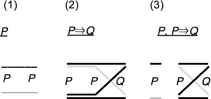

  

  More TD examples

• A connector intersects the nodes at the same level for each instance of the same letter; e.g., in Fig. 10.1 and 10.2 diagonals would be illegal between the Ps.

• The horizontal order of the letters is arbitrary. (Implications of this are elaborated below.)

• Letters in separate TDs are not linked by connectors; e.g., Fig. 10.3.

For ease of interpretation, quaternary and higher arity TDs may be drawn as two (or more) sub-diagrams, with identical orders of letters, but with each sub-diagrams possessing a unique set of connectors that are chosen for convenience. For example, in Fig. 8.4 the right sub-diagram includes connectors that have just one horizontal line running between two neighbouring pairs of variables, and the left sub-diagram has zero, two or three such lines. (Examples below show sub-diagrams with selected sets of connectors actually support interpretation.)

The underlined formula above each TD is a title, and is not strictly a part of the TD.

4.2 Semantics

To explain the semantics of TDs, the graphic elements in Fig. 9 are copied in Fig. 11 and labelled for what they denote:

Fig. 11

Semantics of basic TDs

• Letters are propositional variables (CS1.1).

• Each node represents a truth-value for the variable (CS1.2): high-node T, low-node F (CS1.3).

• The number of the distinct types of variables is the arity of the TD (CS3.2).

• A connector is a case: it constitutes a unique set of truth-value assignments to the variables (CS4.1).

• Connector style represents the overall truth-value assigned to its case (CS4.2). A black connector assigns T: such connectors are “Truth lINES” so are named tines. A grey connector assigns F: being faint they are called faints.

Consider the interpretation of some example connectors in binary and ternary TDs (CS4.3). The top horizontal connector (^{‘–––’}) in Fig. 11.2 is the case P=T, Q=T, which is assigned T. The descending diagonal (‘\’) is case P=T and Q=F, and it is F. In Fig. 11.3, connectors ^{‘––––––’}, ^{‘–––’}\’, ‘\/’ and ‘_ _’ are symbols for TTT, TTF, TFT and FFF, respectively. The top straight tine is T, as is the ‘/\’ tine.

The title of the TD is a suggested interpretation.

4.3 Expressions

TDs are expressively adequate for PL, in the sense that TDs can be generated for any number of variables, and they can encode all possible cases for those variables. Truth values can be assigned to variables in two ways, so a TD for n variables must capture 2ⁿ distinct cases. Each case can be T or F, so ${{2^2}}^{n}$ possible combinations of cases exist for n variables. We show by induction that TDs can encode all possible cases (CS4.1) and all possible combinations of cases (CS4.2) for any number of variables. Imagine a TD for n variables, for example Fig. 12.4 (n=2). To increase the size of the TD by one variable, n+1, we add the variable with its two nodes, Fig. 12.5. Each existing connector must run separately to each new node so we duplicate the original connectors, Fig. 12.6, which doubles their number, and then we complete drawing the new connectors, Fig. 12.7. For our starting case, we can pick Fig. 10.1, a unary TD with one variable, n=1, so there are 2¹=2 cases as required. Thus, by induction, flowing through Fig. 12.2–12.7, a TD of any n will have 2ⁿ cases. Now as a connector may be a just a tine or a faint, the number of combinations of cases is 2 to the power of the number of cases, ${{2^2}}^{n}$, as required.

Fig. 12

Expressive adequacy of TDs

A TD’s pattern of tines and faints expresses a logical relation (CS2.1). Figure 13 shows all four, ${{2^2}}^{1}$, possible unary TDs. (The lines between the TDs and labelled arrows below are explained below.)

Fig. 13

All unary TDs

Figure 14 shows the sixteen, ${{2^2}}^{2}$, possible binary TDs (CS2.1). The title of each is one formula that it represents. The pattern of each TD is a unique iconic symbol for its relation (CS2.1). In particular, TDs of important binary relations are striking patterns: conjunction—top tine only (Fig. 14.1); disjunction—a “stool” (14); implication—‘Z’ (12 or 13); bi-conditional—‘=’ (9); exclusive-or—‘X’ (6); tautology—all tines (15); contradiction—all faints (0). The TDs are arranged in Fig. 14 to reveal various relations among them (CS2.3), and in some ways is a complex analogue to the square of opposition for categorical propositions. The number of tines increases with each successive column of TDs. The TDs on opposites sides of the vertical midline are negations of each other; tines (faints) on one side are faints (tines) on the other (e.g., Fig. 14.0 and 14.15). The TDs along the horizontal midline (14.0, 14.6, 14.9, and 14.15) and at the corners (Fig. 14.1, 14.4, 14.11, and 14.14) are symmetric about their vertical axis, which reflects the commutativity of the represented relations (CS3.3). TDs on opposite sides of the horizontal midline of Fig. 14 are mirror images of each other about their own horizontal midlines (e.g., Fig. 14.11 and 14.14). The lines between pairs of TDs identify inferences, and the classifications at the bottom of the diagram, will be explained below.

Fig. 14

All binary TDs

Ternary TDs have 256, ${{2^2}}^{3}$ = 2⁸, possible permutations of the eight cases. Figure 15 shows four examples. The first two are a ternary conjunction and a ternary disjunction, which distinctively just have a single top tine or just a single bottom faint, respectively; they resemble the equivalent binary TDs (Fig. 14.1 and 14.14). Their symmetry means they also represent (P & Q) & R and (P v Q) v R, respectively, which reflects the associativity of their component binary relations (CS3.3). In contrast, Fig. 15.3 and 15.4 show that the different nesting of the non-associative binary implication operator are dissimilar ternary TDs (CS3.3).

Fig. 15

Some ternary TDs

Figure 8.4 shows one of the 65,536, ${{2^2}}^{4}$ = 2¹⁶, possible quaternary TDs. The pattern of a single top tine or a single bottom faint in binary and ternary TDs holds also for the conjunctive and the disjunctive quaternary TDs, respectively.

4.4 Operators

TD are transformed in various ways, some of which simply change the form of the diagram without affecting the represented relation, whereas others change the form of the TD, the relation among variables and the assignment of truth values to cases.

4.4.1 Letter Operators

The letter relocation operator and the duplicate letter operator work at the level of letters within a TD.

The letter relocation operator exploits the arbitrariness of the relative horizontal location of letters in a TD to sanction the swapping of the position of letters without affecting the interpretation of the TD, provided that the association of connecters with the nodes of each letter remains intact. Figure 16.2 swaps the two variables in Fig. 16.1. Figure 16.3 and 16.4 show relocations of letters in a three letter binary relation.

Fig. 16

Relocation operations

The letter duplication operator introduces an additional copy (or copies) of an existing letter, exploiting the idea that a variable may be represented by one or more letters in a single TD. This is permissible provided that the connectors associated with the original letter are also duplicated. For example, we duplicate P in Fig. 16.1 to get Fig. 16.3 (or Fig. 16.4). Complementarily, this operator permits the erasure of duplicate letters.

These purely syntactic operators usefully transform the surface form of TDs into alternative patterns that may be easier to interpret visually, in order to support the making of inferences (see below).

4.4.2 Heuristic Negation Rules

Two heuristic negation operators are defined. A formal negation rule follows below. The TD negation rule switches the tines of a single TD to faints, and faints to tines, to negate the TD. For example, compare the TDs on opposite sides of Fig. 14. The variable negation rule, works at the level of individual variables. In order to formally construct a TD containing a negated variable, one would first draw the TD for that variable, apply the negation operator to it (see below), and then compose the desired TD. Alternatively, we make take a TD that contains the variable in un-negated form and (for all occurrences of the target letter) simply swap the vertical position of its nodes with their connectors attached. For example, this rule transforms Fig. 14.12–14.14, with the negation of P.

4.4.3 Composition Operators

TD-operators compose given argument TDs to generate result a TD (CS3.1). Figure 17 shows examples of unary, binary and ternary TD-operators (CS3.2). We first consider the structure of TD-operators; Fig. 18 names their components.

Fig. 17

TD-operators for composition: 1–4 unary; 5–8 binary; 9–11 ternary

Fig. 18

Components of 1 unary and 2 binary TD-operators

• TD-operators are drawn within a dotted-line rectangle.

• TD-operators have one or more inputs, which each consist of two lines, one tine above and one faint below a lower-case letter ‘a’. The number of inputs is the arity of the TD-operator, and numbered subscripts distinguish the two or more inputs.

• A TD-operator has one output consisting of a pattern of tines and faints. For a given arity, the pattern is the same as the configuration of connectors in a basic TD. The ends (and intermediate points) of each output line is associated with a unique combination of tines and faints of the input lines.

• The specific pattern of output line styles defines the nature of the operator, as in the examples in Fig. 17.

• The application of a TD-operator matches the styles of connectors for a given case in the argument TDs to its inputs and uses its output line styles to determine the style of the result connectors for that case.

Applying a TD-operator involves four steps, which are illustrated in Figs. 19 and 20.

Fig. 19

Unary TD-operator in action

Fig. 20

Binary TD-operator in action

• (S1) The arity of the result TD equals the number of distinct variables in the arguments. For example, applying a binary operator to a TD in P and Q and a TD in Q and R would generate a ternary TD in P, Q and R.

• (S2) Pick one case, select connectors in the argument(s) for that case and identify the connector in the result that matches the case (connectors run to equivalent nodes for each variable in the argument and result).

• (S3) For the case in S2, use the styles of the argument connectors as inputs to look up the output style, as described above.

• (S4) Apply the style found in step S3 to the result connector identified in step S2.

Steps (2) to (4) are repeated for every case.

Figure 19 shows the application of the negation TD-operator to the high node of TD ¬P. (S1) As the argument is unary, the arity of the result will be one. (S2) Take P’s high node case, for example. (S3) Its connector is a faint, so this is the input to the TD-operator. (S4) The corresponding output style is a tine, so the connector in the result TD becomes a tine. Repeating steps S2 to S4 produces a faint for the other (low-node) case (not shown in Fig. 19). The pattern of connectors in the result is the TD for P.

Figure 20 applies the disjunction binary operator to unary TDs ¬P and Q. (S1) The two variables in the arguments make TD binary result (Fig. 20.1). (S2) Pick, for example, the low-node connectors in both arguments, which matches the bottom connector in the result TD (Fig. 20.2). (S3) The P connector is a tine and the Q connector is a faint, so these are the inputs (Fig. 20.3). (S4) The corresponding result is a tine, so the bottom connector of the result TD is drawn as a tine (Fig. 20.3). Figure 20.4 shows steps S3 to S4 for the high-node P and the low-node Q, which yields the \ faint in the result. The other two cases follow in a similar manner (e.g., Fig. 20.4).

The patterns of lines in the disjunction, conjunction and bi-conditional TD-operators are symmetric (Fig. 17.5, 17.6 and 17.8), so the connector patterns they produce is independent of the order of the arguments, whereas the implication operator is asymmetric so is not commutative (Fig. 17.7). The design of the binary TD-operators deliberately reflects the structure of the binary relations (cf. Figure 17.5–17.8 and Fig. 14.9, 14.11, 14.12, and 14.14). This suggests that other operators could be defined using any of the TD patterns in Fig. 14 (CS3.4); an idea taken up below.

Figure 21 shows the application of disjunction, implication and conjunction operators to various TDs. Here, the arguments and operators are at the top and the results are below, but graphical devices other than spatial layout may be used to show such constructions. The TD-operators are elevated above the mid line of the arguments TDs to reinforce the idea that step S3 applies the operator patterns to the styles of the connectors (and not to their shapes). Users familiar with TD-operators may simply draw the pattern of lines in the dotted rectangle and omit all the other symbols (e.g., Fig. 21.3). In Fig. 21.1 two binary argument TDs share variables, so the result TD contains the same variables and the configuration of connectors is identical to the arguments. Combining of a unary and binary TDs with different variables result in a ternary TD, Fig. 21.2, and the eight connectors of the result TD are generated by combining the high and low connectors of P separately with all four connectors in the binary TD. Exceptionally the lines have been coloured to show their origin; grey for P and green for Q & R. Figure 21.3 provides a contrast with two binary argument TDs sharing one variable, P. As step S2 deals with cases, connectors are only combined when they are at the same node in P, so the resulting ternary has just eight connectors, and not sixteen, even though each argument has four connectors. Again colour shows the origin of the parts of the result connectors.

Fig. 21

TD compositions: 1 (P v Q) v (P & Q), 2P ⇒ (Q & R); 3 (P ⇒ Q) & (P ⇒ R)

4.4.4 Heuristic Composition Rules

The formal application of TD-operators is rather laborious, so quick and simple heuristic rules have been devised. For each binary operator two complementary heuristics are feasible, each succinctly specifying the input conditions for which the output is a tine or a faint. Consider the conjunction operator, Fig. 17.5: a result connector is a tine just when both argument connectors are tines, and a result connector is a faint whenever one or both argument connectors is a faint. For example, in Fig. 21.3, five tines and three faints are given by the two rules, respectively.

Similar rules for disjunction, implication and bi-implication follow by inspection of Fig. 17.6, 17.7 and 17.8.

4.4.5 Decomposition Operators

Decomposition operators work like composition operators with a focus on the connector styles associated with cases, but they split apart one of the argument TDs. Figure 22 shows two examples. The first operator takes an argument TD, a₁ (e.g., a P, Q and R ternary), which could have been assembled from two parts, a_1A (P and Q binary) and a_1B (unary R), whose joint pattern of connectors matches the input pattern to the left of the operator (in the dotted rectangle). The result, r, is one of those potential components, r=a_1A (which happens to be the bi-implication in P and Q). Figure 22.2 is an example with an operator that we will call v-decom, which takes two argument TDs, one of which can be imagined as two parts, a_1A–a_1B (P, and QvR), whose assembly conforms to the pattern to the left of the operator. The other TD, ¬a_1A right (¬P), is the negation of the first of the two parts. From this, the second of the two parts can be obtained, a_1B (QvR). Given an applicable operator for the selected TDs, the application of the decomposition operators follows steps similar to S1-S4, but a preliminary step is needed to find a matching operator for the given TDs.

Fig. 22

Decomposition operators

Composition and decomposition operators generate new TDs, but they are not necessarily valid inferences. The revealing connections between these operators, validity and the rules of natural deduction are considered below.

4.4.6 Connector-Style Operator

This final class of operators is special, because it contains a single deceptively powerful operation. The connector-style operator relies on the TDs defining a relation among variables as a particular pattern of connectors. Changing the style of one connector, or more, changes the encoded relation; therefore, a new relation can be obtained from any other merely by changing connector styles (for example, jumping around Fig. 14). Of course, the question is to specify conditions under which this operator can be meaningfully and validly applied. Such conditions are examined below.

4.5 Meta Truth Diagrams

TDs have so far been presented at a concrete level with expressions including all the cases in relations. However, this amount of detail can be cumbersome and mask higher level relations and ideas. So, this sub-section introduces Meta-Truth Diagrams (CS6.1); see Fig. 23.

Fig. 23

Meta-TDs

• Meta-TDs have bold capital letters as meta variables for propositional relations.

• A meta-TD is drawn with such letters above a pattern of connectors.

• A meta-TD represents a TD, which may have any arity.

• Tines and faints in a meta-TD represent sets of tines or sets of faints in the denoted TD: e.g., the faint of B in Fig. 23.2a represents the three faints in Fig. 23.2b.

• The configuration of lines in a meta-TD is the same as the configuration of connectors of a basic TD with that same number of variables.

• High nodes record the occurrence of tines, and low nodes faints, in the represented TD (rather than assigning truth values to propositional variables).

• A unary meta-TD can represent a given higher arity meta-TD, where its tine (faint) incorporates all the tines (faints) in the sets of TDs of the given meta-TD; for example, Fig. 23.3a.

• Binary (and higher arity) meta-TDs represent the outcome of composing two (or more) argument TDs into a new TD, where each meta-variable is an argument TD and the pattern of connectors reflects how combinations of the styles of (sets of) argument connectors produce the specific styles of (sets of) result connectors. For example, Fig. 23.3c is the result of the application of the implication operator to two TDs, see Fig. 21.2, so the Z pattern of tines in the meta-TD shows they were produced by that operator (e.g., in Fig. 21.2, when P’s tine is combined with the faints in Q & R by the implication operator (Fig. 17.7) a faint is produced, hence the descending connector Fig. 23.3b). In general, patterns of connectors of a higher level meta-TD will be the same as the pattern of lines in the operator.

That completes the introduction of TDs, their operators and how to express TD relations in general through meta-TDs. Together the TDs, so far, satisfy the first 17 conceptual scope criteria.

5 Validity, Inference and Proofs

Many operators for generating TDs were described above. This section considers: the nature of valid inferences and proofs using TD; how TDs may support the demonstration that particular systems of PL are sound and complete; and, general explanations about the nature of PL. All of this is underpinned by the test of validity that TDs provide.

5.1 Validity Test

In PL a premise validly implies a conclusion when a case of a premise is true and for that case the conclusion is also true. Equivalently, for an inference to be valid, no false case in a conclusion may be associated with a true case in the premise. Wittgenstein (1961) and others (Post 1921) devised truth tables as a tool to operationalise this definition.

The TDs provide a diagrammatic method to evaluate inferences by comparing the style of connectors in the premise TD(s) with those in the conclusion TD (CS5.3). The method uses to two additional types of TDs — the TD-test and the validity-TD, Fig. 24.

Fig. 24

The components of the TD-test and validity-TD

• The TD-test and validity-TD are drawn with a rectangle with a solid perimeter. Just one or both may be included.

• The TD-test is applied to a premise(s) and a conclusion in a similar fashion to the application of a TD-operator to arguments. The output of the TD-test is a validity-TD, which is akin to the result of a TD-operator.

• In the TD-test, ‘p_1,n’ stands for all (1 to n) premise TDs (or meta-TDs) in the inference and ‘c’ stands for the conclusion TD (or meta-TD).

• The high nodes (‘All —’) of p_1,n refers to cases in which the connectors of all the premises are tines.

• The bottom nodes (‘≥1 —’) refers to all other cases in which at least one faint is present among the premises.

• The high and low nodes of ‘c’ refer to cases in which the conclusion is a tine or a faint, respectively.

• The pattern of lines in the middle determines the validity status of matching cases in the premise(s) and conclusion, by comparing their styles. Solid lines are validity lines and dashed lines are invalidity lines (they are not tines and faints, because they do not encode the assignment of truth-values). V1, V2, V3 and Vx identify three valid conditions and one invalid condition, respectively (Fig. 24).

  • V1 (^–––): all the premise connectors are true and the conclusion is true.

  • V2, (_–––): at least one premise is false and the conclusion is true.

  • V3, (/): at least one premise is false and the conclusion is false

  • Vx, (\): all the premise connectors are true and the conclusion is false.

• The validity-TD includes all the variables (meta-variables) in the premise and conclusion (CS5.4).

• A validity-TD’s configuration of connectors is that of a basic TD with the same arity.

• The style of its connectors are given by the outcomes of the validity test.

• An inference is valid when the status of all the cases is valid; i.e., all the validity-TD lines are solid.

Figure 25 shows tests of two example inferences. The dotted vertical line separates the premise and conclusion TDs. Figure 25.1 shows that a proposition validly implies itself: the TD-test condition V1 matches the premise tine to the conclusion tine (high-nodes); similarly, V2 matches the faint in the premise to the conclusion faint (low-nodes). In Fig. 25.2 we cannot infer an implication from a reverse implication of the same variables. The tine / connector in the premise and the faint / connector in the conclusion is a Vx. The TD-test works on inferences with different numbers of variables in the premises and the conclusion.

Fig. 25

Examples of TD-tests and validity-TDs for two inferences

The application of the TD-test to every one of the cases in an inference is potentially laborious, especially for ternary and higher arity TDs. Fortunately, a heuristic rule simplifies the application of the TD-test:

• Validity-rule. An inference is invalid if there is any faint in the conclusion whose case just possesses tines in the premises (Vx); otherwise the inference is valid.

The validity-rule can (often) be applied by inspection (CS5.3, CS5.4). And, the symmetry of some TDs and the flexibility of their layout can sometimes expedite the application of the validity-rule. Further, when one applies the validity-rule, or is familiar with the TD-test, the TD-test diagram may be omitted from the rectangle and just the validity-TD drawn.

The TD-test refers to multiple premises, although the common definition of validity, as stated above, applies to a single premise. So, we must show that the TD-test is valid for any number of premises, that is prove its monotonicity: in effect we prove the rule of assumption is valid. This we do by using the meta-TDs and induction. Figure 26.1 depicts a valid inference from premise B to A, which may be any arbitrarily complex relations. As the inference is valid, no tine in the premise results in a conclusion faint, by the validity-rule, so the validity-TD excludes condition Vx, shown by a dotted line. Now we add another premise C, Fig. 26.2, and consider all cases involving all combination of tines and faints across the three TDs in the ternary validity-TD. However, we know that no cases that include B and ¬A exist (dotted B\A connector), so two ternary connectors are prohibited, as shown by the dotted lines. Considering all the other cases, one of the valid conditions always applies, so the inference is valid. If we add a further TD, D, again the inference cannot be invalid, because cases for C, B and ¬A are excluded so no D^–––C^–––B\A cases can be generated. Further, TDs can be added ad infinitum, so the TD-test is generally valid for any number of premises.

Fig. 26

Validity of the TD-validity test

5.2 Valid Inferences

We will now use the TD-test to examine the validity of operators and inferences.

5.2.1 Equivalence

The TD-test tells us that if a premise TD and a conclusion TD for the same variables are generated by different compositions that yield identical TDs (same pattern of connectors), then the conclusion is valid to infer from the premise, and also vice versa, because validity conditions V1 and V2 apply exclusively for all cases between the premise and conclusion. As heuristic negation rules can be used to interpret different relations form the same TD, we may infer the equivalence of certain relations. For example, the stool pattern in Fig. 14.14 may be transformed in to a Z pattern by applying the variable-negation rule to P, and as the Z pattern is implication, Fig. 14.12, we have shown that P⇒Q is equivalent to ¬PvQ. Similarly, using both heuristic negation rules, we can show that ¬(P & ¬Q) is also equivalent to P ⇒ Q, because they have similar patterns of connectors.

5.2.2 Valid Operators and Natural Inference Rules

The TD-test determines which of the TD-composition and decomposition rules are actually valid, by checking that each case with a faint in the conclusion does not exclusively possess tines in the arguments. This provides a framework for examining the rules of natural deduction, as all but one can be interpreted as TD compositions or decompositions that happen to be valid. Conjunction introduction (e.g. Fig. 21.3), disjunction introduction (Fig. 21.1) and assumption are TD compositions, and double negation is two compositions. Modus ponens, modus tollens, conjunction elimination, disjunction elimination and reductio ad absurdum are decompositions (when sub-proofs in the latter two are treated as implications). For example, Fig. 27 shows an example of how the application of the Modus ponens splits an implication relation expressed in meta-TDs. Applying the validity-rule (or TD-test in full) to these operations shows that they are valid. For example, Modus Ponens, Fig. 27, expresses the rule A ⇒ B, A ⊢ B. B is rightly concluded, because the faint in B is never associated just with premise tines (i.e., B’s ‘_’ faint is either associated with the ‘\’ faint of A ⇒ B, or with the ‘_’ faint of A).

Fig. 27

Modus ponens

The conditional proof is special because it includes sub-proof, from which an implication relation is inferred. (Obviously, the sub-proof cannot be replaced by an implication relation, unlike the other rules with sub-proofs.) To demonstrate the validity of this rule requires two applications of the validity-rule, see Fig. 28. First, assume that n+1 assumptions validly implies C (Fig. 28.1). For this to be true, those (sets of) cases which are all tines in the premises must not match a faint in the conclusion, as shown by the thick grey line, and the dotted line in the validity-TD. Now, we form a new inference with a conclusion where one of the assumptions (A_n+1) implies C, with a Z pattern of connectors (Fig. 28.2). Applying the validity-rule we see that the only cases where a faint in the new conclusion could match just tines among the assumptions has been excluded by the first step. Note the similarity in structure to Fig. 26, which demonstrated validity of the validity-test for multiple TDs. This approach can also be used to show the validity disjunction elimination and reductio ad absurdum when they are expressed with sub-proofs rather than implications. In general, we may interpret the role of the sub-proofs in rules as establishing pre-conditions that exclude certain cases that would otherwise cause the rule to fail.

Fig. 28

Validity test of conditional proof rule

Basic TDs and valid TD-operators may of course be used in place of the formulas in proofs such as Fig. 1. Alternatively, the TDs can be organised as nodes in a lattice to usefully visualize the structure of proofs. The top nodes of the lattice are the premise TDs and valid TD-operators are applied by pattern matching on those and later nodes. A proof is successful when the lattice is brought together in a single conclusion node, with no loose branches, which shows that the assumptions are discharged. Such lattices neatly depict the overall structure of natural deduction proofs and allows different strategies to be formulated and compared.

5.2.3 Applying Connector-Style Inferences

Connector-style operators, as described above, change the style of connectors to express alternative relations. Returning to the four unary TDs in Fig. 13, each of the lines between pairs of TDs represents a single application of a connector-style operator to one connector. From the validity rule, each line going rightward represents a valid inference, because no case has a tine implying a faint. Similarly, in Fig. 14, as the number of tines increases monotonically along rightward paths across the diagram, each line is a valid inference. The premise at the beginning of a line has no cases with faint connectors that match to tines in the conclusion at the line’s end. Further, any continuous multistep rightward path also represents a valid inference from the TD at its start to the TD at its end. The longest path captures the idea a contradiction implies a tautology. Figures 13 and 14 embodies an important general interpretive scheme provided by TDs, whereby related TDs may be organised from a contradiction on the left to a tautology on the right with all valid inferences represented by rightward pointing edges (or invalid inferences by leftward edges). We will use this interpretive scheme in the proof of the completeness of the TD system below.

Combining connector-style operators with equivalences (Sect. 5.2.1) provides a powerful TD inferential system. For example, consider Leibnitz’s ‘splendid’ theorem: ((P ⇒ R) & (Q ⇒ S)) ⇒ ((P & Q) ⇒ (R & S)). Sowa (2008) reports Whitehead and Russell required 43 steps to prove this theorem in Principia Mathematica, but Sowa (2008) gives a proof in just seven steps using Alpha Graphs. Let us consider the harder task of not just showing the validity of the theorem but discovering another conclusion that can be derived from the same premise. Discovery is more challenging than proof because we are not given a target conclusion that provides clues for selecting a proof strategy.

Figure 29.1 is a quaternary TD for the conjunction of the two implications on the left of the theorem, which is drawn with Q and S reversed in order to exploit symmetry to aid the process of drawing. The conjunction operator and the two implication relations are shown in the middle of Fig. 29.1, and all the resulting tines for the quaternary are gathered on the left and all the faints on the right. Connectors with similar configurations are coloured merely to aid reading. To find valid conclusions we seek meaningful patterns of connectors that do not increase the numbers of faints (cf. Figure 14). Our approach is to selected some subset of premise faints to keep as faints in the conclusion and to make all other conclusion connectors tines: so we focus on the right of Fig. 29.1. Inspecting the faints, it is clear that P and Q have similar patterns to each other, and similarly for R and S, which suggest that some symmetric relation governs each pair. So, the pattern of faints is redrawn using a letter relocation operator to give Fig. 29.2. A pattern of three P^–––Q faints connected to an inverted stool of R and S is now one apparent pattern, extracted in Fig. 29.4, which suggest that some combination of conjunction or disjunction of binaries that are negated or inverted may be the constituents of a conclusion TD. Remember, these connectors are to be faints in the conclusion and that the implication operator (Fig. 17.7) produces a faint when combining a tine and a faint, so the pattern of faints in Fig. 29.4 can be produced by an implication over two conjunctions: the ^––– tine of P and Q combines with the /, ^––– and \ faints of R and S to give the three required faints, Fig. 29.3. Thus, we have shown that (P ⇒ R) & (Q ⇒ S) implies (P & Q) ⇒ (R & S). Further, there is a complementary pattern of three faints in the premise, Fig. 29.6, so by similar reasoning we have discovered another conclusion but with an implication of two disjunctions, Fig. 29.5, that is (PvQ) ⇒ (RvS).

Fig. 29

What can we conclude from (P ⇒ R) & (Q ⇒ S)?

The example shows how TDs can be used for proofs but also to discover theorems in the first place. Finding valid inferences can also proceed in the opposite direction by looking for patterns that increase the number of faints in the premise (cf. moving right to left, in Fig. 14). Satisfying the validity-test guarantees that an inference will be valid, but will we always be able to find some meaningful relation for every pattern of connectors (e.g., set of binary formulas)? Yes. A relation can always be formulated, because a TD can be composed from a disjunction of conjunctions for each tine in a TD (e.g., Fig. 14.11 from Fig. 14.2, 14.3 and 14.4). In other words, any TD may be read as a disjunctive normal form expression (or focussing on faints, as a conjunctive normal form expression).

5.3 Soundness and Completeness

Is the TD approach logically sound and complete (CS6.2)? This question may be framed in two ways. First, we might use the TD system to represent selected logical relations and inferences that are used by some other notation and then ask whether that specific particular formulation of PL is sound and complete (adequate). Alternatively, we may ask whether TDs are in themselves adequate just on the basis of selected diagrammatic TD rules. Each is considered in turn.

If a TD system for PL is restricted to unary and binary relations and adopts the laws of natural deduction, the system is equivalent to that version of the formula notation, so would inherit soundness and completeness merely by translating to the formula notation at the start of its proofs and translating back to TDs at the end. But such a proof of adequacy is a representational sleight of hand. The adequacy of a TD formulation of PL can be performed wholly using TDs. Consider, for instance, natural deduction. The soundness of the laws is established by showing that each rule is valid for any suitable premises. Meta-TDs are used for this purpose. In Sect. 4.5 we saw that a meta-TD can represent any basic TD, because its connectors stand for sets of tines or faints in basic TDs (see Fig. 23). Thus, a demonstration that an inference expressed using meta-TDs, using the validity-rule, shows, in effect, that all inferences in basic TDs, which are expressible by the meta-TDs, are also valid. For example, the Modus Ponens inference in Fig. 27 is stated using meta-TDs and was shown to be valid. The meta-TDs may be replaced with the specific TDs shown in Fig. 23.1b, 23.2b and 23.3c, which preserve the implication relation. But as the tine and faint connectors in the meta-TDs stand for any set of tines or faints, then any other set of TDs that preserve the implication may be substituted, and will also be valid. Hence, Modus Ponens is generally valid. The same reasoning can be applied to the soundness of all natural deduction rules.

Turning to completeness, a fully diagrammatic proof in TDs can be made by using TDs in place of formulas in all the steps of a formula based proof. All sentential meta-variables are replaced by meta-TDs, conventional operators by TD-operators, and the inference rules by TD versions of those rules. Further, a proof in the sentential notation may be recast as a lattice, with TDs at the nodes, and edges standing for inferences. Combining the visual form of TDs with the 2D spatial layouts of proof structures may aid our comprehension of the trickier steps of a completeness proof by exposing the underpinning function of complex sequences of inferences. For instance, a TD reproduction of Lemmon’s (1965) proof of completeness reveals how nested applications of disjunction eliminations are used, in a specific nested pairwise combinatorial fashion, to reduce to a single thread the multiple parallel lines of inference, which were each initiated by the proof’s many initial assumptions. In summary, the adequacy of a system of PL may be established using TDs to replicate a proof taken from a conventional notation.

Our second question about adequacy is whether a purely TD approach can establish the soundness and completeness of TDs in general. In other words, is it possible to generate all possible ordered sequences of TDs, of any arbitrary complexity, where the last member of the sequence is validly implied by all the previous members? In particular, is this feasible just using connector style operators (Sect. 4.4.6) and the rule of assumption?

For these proofs a final type of TD is introduced to encode inferences. An inference-TD consists of (a) bold capital letters P and C to denote the premise(s) and the conclusion (C), respectively, and (b) pairs of lines above the letters. All fifteen possible inferences-TDs are shown in Fig. 30 (labelled A–O). A line in a pair is either black or grey (in the text shown as ‘—’ or ‘–’). Each line represents a set of connectors, like meta-TDs, the but with special restrictions. First, the lines are considered in pairs (e.g., ‘–:–’ and ‘—:–’ in Fig. 30C). Second, each pair represents a set of cases which have certain assignments of tines or faints to the premise and conclusion connectors, specifically:

Fig. 30

Relations between inference-TDs

• 1. ‘—:—’ = cases with tine premise connectors and tine conclusion connectors (valid).

• 2. ‘–:—’ = cases with faint premise connectors and tine conclusion connectors (valid).

• 3. ‘—:–’ = cases with tine premise connectors and faint conclusion connectors (invalid).

• 4. ‘–:–’ = cases with faint premise connectors and faint conclusion connectors (valid).

An inference-TD may include between one to four pairs. All possible combinations of pairs are shown in Fig. 30A–O, but the five central inference-TDs are not applicable to unary TDs because they only have two connectors. (Purely to ease comparisons between inference-TDs, each type of pair has a given specific location above the letters; e.g., –:– at the bottom.)

Consider some examples with reference to Figs. 13 and 14. An inference-TD with just one pair (A, E, K, N) represents an inference in which all the cases possess the same pattern of assignment of connector styles, for instance Fig. 30A represents a contradiction implying a contradiction (e.g., Fig. 13.0 ⇒ 13.0; Fig. 14.0 ⇒ 14.0). Figure 30.B represents Fig. 13.0 implying 13.1, or 13.0 ⇒ 13.2: as noted by the ‘B’ arrow in Fig. 13. And similarly with Fig. 14.0 implying 14.1 to 14.4. Figure 30.M represents inferences to the tautology Fig. 13.3 from either 13.1 or 13.2—L arrow. And similarly Fig. 14.15 from 14.11 to 14.14. Figure 30O represents a tautology implying itself. Inference-TD Fig. 30G with three pairs represents any of the rightward inferences between TDs in the middle four columns in Fig. 14 (e.g., 14.1 ⇒ 14.6, or 14.5 ⇒ 14.13)–G arrows.

In general, Fig. 30 applies to inferences in which at least one TD is not a unary. For exclusively unary TDs, the middle five inferences with three or four pairs are omitted.

Let us now define valid inferences with connector-style operators. From the validity-rule any inference that includes any combination of pairs (1), (2) or (4) is valid, but any that includes pair (3) must be invalid, because it would violate the TD-test. The valid inference-TDs have solid perimeters (none of them include a —:– pair) and invalid inferences have grey backgrounds (all include a —:– pair). Hence, the soundness of TDs follows automatically, because all inferences using valid connector-style changes are valid by definition. The greater challenge is completeness.

For completeness it must be shown that all valid inferences can be derived using the valid connector-style rules and the rule of assumption. The proof has two stages.

The overall strategy of the first stage involves starting with an inference that is known to be valid and showing that any other valid inference, whatsoever, can be obtained just by applying valid connector-style operators. We start with the inference that a contradiction validly implies itself, Fig. 30A. So, we must show that all valid patterns of inference can be generated stepwise from inference-TD 30A, until we reach the inference that tautology validly implies itself, Fig. 30O. To support this, Fig. 30 has been arranged consistently with our overarching TD interpretive scheme (cf. Figures 13 and 14). More specifically, we must show (step 1) that each inference-TD in Fig. 30 represents all possible valid premise-conclusion associations of that type, and (step 2) that all inference-TD can be found from a previously established inference-TD, using just connector-style operators. The two steps are considered in turn.

Step 1 (of stage 1)—intra inference-TD transformations. For unary TDs step 1 can be achieved by simply enumerating all nine valid inferences implicit in Fig. 13 and matching them to Fig. 30’s inference-TDs (i.e., 30A—13.0 ⇒ 13.0; 30B—13.0 ⇒ 13.1 or 13.0 ⇒ 13.2; 30E—13.0 ⇒ 13.3; 30F—13.1 ⇒ 13.1 or 13.2 ⇒ 13.2; 30M—13.1 ⇒ 13.3, 13.2 ⇒ 13.3; 30O—13.3 ⇒ 13.3). For other arities we note that Fig. 30 includes all possible inference-TDs, and the subset of valid inferences are unambiguous, so we have an exclusive set of valid patterns of inferences. Now, does each valid inference-TD represent all possible inferences within its set of connector patterns? Remember, that a line in an inference-TD represents a set of cases with connectors of the same style. Thus, each pair can represent between (i) one case and (ii) the total number of cases minus the number of other pairs (i.e., (i) for other pairs). For example, as noted above, Fig. 30G represents all of the rightward inferences among the inference-TDs of the four middle columns of Fig. 14; every pair has between 1 and 2 cases (i.e., 4 cases minus 1 case for each of the two other pairs). Applying the connector style-operator to the premise or conclusion side of a case swaps the style of the connector, and provided that the operation matches one of the pairs in the chosen inference TD and is within the give numerical limits, any connector whatsoever may be changed (e.g., the transformation of inference Fig. 14.1 ⇒ 14.9 to inference 14.9 ⇒ 14.13 involves swaps of faints to tines in different cases). This process may be repeated for any other connector as desired, therefore all possible combinations of connectors permitted by the set of pairs in a given inference-TD can be generated incrementally.

Step 2—inter inference-TD transformations. In this step it must be shown that all the valid types of inference-TDs can be obtained by connector style changes to either a premise or a conclusion connector. The permitted transitions are shown by the (thick) lines between pairs of valid inference-TDs in Fig. 30, which are of three types: (a) the introduction of new pair (e.g., from Fig. 30B–G); (b) elimination of an existing pair (e.g., 30G–30M); (c) the simultaneous occurrence of both (e.g., 30B–30F). All the possible transitions have been enumerated in Fig. 30. All the transitions (green and red lines) are applicable to binary and higher arity TDs, but only the transition involving one or two pairs are applicable to unary TDs (red lines). By inspection of Fig. 30, it is clear all valid inference-TDs can be reached from the initial contradiction inference-TD by following exclusively valid transitions, and similarly the tautology inference can be reached from all valid inferences. This is true for unary and higher arity TDs. Thus, summarising both steps of stage 1, all possible valid inferences between a single premise and conclusion can be found by applying connector-style operators.

The second stage of the proof generalises the result just obtained to inferences with any number of premises. The strategy here resembles the strategy used to show that the validity-TD can be extended from a single premise to multi-premise inferences (end of Sect. 5.1). Inference-TDs are extended by further refining the permitted interpretation of the premise lines in the pairs so that the validity rule holds for multi-premise inferences: if a conclusion connector is a faint, the case is valid so long as at least one of its premise connectors is also a faint. Thus, the left lines in the four definitions of pairs, above, are taken to represent all the connectors across the multiple premises of each case, with a grey line then denoting cases in which at least one connector is a faint, and a black line denoting cases in which all the connectors are tines. With these changes, the style-operators can be applied in isolation to any one of the component premises within a multi premise inference, which means Fig. 30 is still applicable. For example, imagine that the –:— pair in Fig. 30M represents just one case in which some premises have faint connecters. Now if each of those faints is changed to a tine, one by one, using the style operator we would have new inferences but not change the type of inference (still Fig. 30M). However, when the last faint in the premises is changed to a tine, we no longer have a –:— pair, so the new inference Fig. 30O is then produced. Thus, all valid multi-premise inferences can be found.

That completes both stages of the proof of completeness, hence it has been shown that the TD system is both sound and complete. This in turn concludes our overview of TDs’ coverage of the PL conceptual scope criteria.

6 Discussion

Truth Diagrams, TDs, provide a range of diagrammatic components for the representation of PL. A particular limitation of the system is the difficulty of drawing TDs with more than three variables, which requires the introduction of supplementary drawing techniques not specifically related to the underlying syntax and semantics of the system. However, reviewing the seven previous representations, cumbersome expressions or bulky sets of expressions appear to be unavoidable for a domain of the complexity of PL (cf. Figures 1, 2.5, 3.6, 4.3, 5.3, 6.10, 7.11). So, the critical epistemic question is how much content does each representation successfully encode given its relative complexity.

The conceptual scope criteria were formulated to systematically compare our representations’ coverage of the key ideas of PL. TDs address the criteria more fully than the formula notation, truth tables, Venn diagrams, Frege’s conceptual notation, Wittgenstein’s diagrams, Gardner’s shuttle networks and Pierce’s Alpha graphs. In particular, it is superior with regard to the later criteria relating to the general nature of PL. This section considers the relative merit of TDs versus the other representations, and consequently reveals that some concepts which are seemingly central to PL are actually idiosyncratic aspects of particular representations.

TDs appear to make the underpinning coherence of PL more readily apparent than the other notations, because it provides related notational devices to connect key ideas (CS8.1). The Z shape pattern of tines and faints shows that the (binary) implication relation (Fig. 14.12), the implication operator (Fig. 17.7), the TD-test and validity-TD (Fig. 24), the validity-test, modus tollens and modus ponens (Fig. 27), and the conditional proof inference (Fig. 28) are all linked concepts and closely associated with the specific definition of validity that prohibits false statements being legally deduced from true statements (i.e., the \ faint in the Z pattern). The other representations tend to mask this unifying conceptual thread.

TDs show, at a fundamental level, that truth and falsehood are fully complementary in PL (CS8.3): the high and low nodes, and the alternative styles of connectors, are complementary. One could perversely but legitimately discuss PL largely in terms of maintaining falsehood or deriving invalid inferences. However, this fundamental symmetry is not revealed by the basic form of the formula notation, Frege’s notation and Pierce’s graphs: it is hidden by the use of representational devices specific to negation (¬, vertical tick (Fig. 3.2), and cuts (Fig. 7), respectively). The other representations do treat T and F symmetrically, like TDs. Interestingly, what breaks the underlying symmetry is the definition of validity, which places restrictions on when true proposition may contribute to a valid inference—the ubiquitous Z pattern is asymmetric. TDs can support the exploration of PL systems with alternative definitions of validity merely by swapping the Z in the validity-test for any of the other patterns in Fig. 14 (CS8.4). How would PL work with validity based on bi-implication, conjunction or disjunction (Figs. 14.1, 14.9, 14.14)?

PL texts often justify rules of inference by appealing to our experience. Alternatively, truth tables (e.g., Fig. 2.1–4) are used to circumvent learner’s intuitive concerns about the nature of implication (CS7.1), although none of our sample texts use them to test the validity of the core inference rules, nor to show that key counter intuitive inferences are valid, or that others are invalid (CS7.2, CS7.3). Perhaps, little additional insight can be gained from mechanically conducting such tests with truth tables. In contrast, the validity-TD does not just determine validity but also reveals the circumstances, cases, that contribute to the legitimacy of an inference (e.g., Figs. 25, 20, 28). This exemplifies how TDs can be used to explain how the other representations work (CS9). Many of the TD examples above may be interpreted as explanations of concepts and inferences normally presented in the formula notation. An attractive feature of Peirce’s system is its relatively small number of inference rules (Fig. 7), which can generate proofs with fewer steps than the formula notation. However, explanations of why the rules work are not typically provided in accounts of that system. TDs can explain why Peirce’s rules work (CS9). For instance, by modelling the rule of insertion with TDs (Fig. 7.9), we see that the process of drawing the conjunction of an existing TD (e.g., P, in Fig. 7.9) with a new TD (Q), and then swapping all the styles of all the connectors to negate the composite, necessarily produces just tines in the new TD to match the tines in the initial TD, so ensuring validity.

The formula notation possesses just unary and binary operators, but the absence of higher arity operators is not a fundamental feature of PL. Rather, it is a characteristic of the linear syntax of that notation (CS8.2): an operator symbol cannot be written between three letters without changing the basic form of the notation (e.g., to a prefix format). TDs and Pierce’s graphs express higher order operations, in interestingly different ways. Pierce’s rules apply to subgraphs in general, without particular reference to specific numbers of variables. TD operators have specific arities, but the arity is not limited. In the way that TDs for ternary operators, such as Fig. 17.9–11, can be defined from basic TDs for ternary relations, Fig. 15.1–3, respectively, higher order operators can be defined using their respective TDs.

The importance of the connection between truth-value assignments, the truth of relations and the validity of inferences is acknowledged in PL texts (CS5.4). A critical distinction is the difference between the assignment of truth values to variables and the assignment of truth values to the specific cases of a relation. The formula notation, Frege’s notation, Venn diagrams and Peirce’s graphs do not in themselves make such assignments. Truth tables do deal with both types of value assignment, but tend to obscure the distinction by mixing together columns for assignments of values with columns for assignments to relations. Similarly, Wittgenstein’s diagrams use one graphical technique for both types of assignment (i.e., lines to T and F labels). In contrast, Gardner (1958) explicitly designed his network representation to preserve the distinction—vertical T and F lines versus horizontal shuttles. Likewise, TDs differentiate the types of assignment by the position of a variable’s nodes versus the style of connectors, respectively. The clean separation of types of assignments underpins the definition of meta-TDs, which in turn enables TDs support higher level reasoning about the nature of PL.

TDs are preferable to shuttle diagrams, for various reasons, even just at the level of expressing relations. First, the range of TD patterns are more distinctive, iconic, than shuttle diagrams, because TDs exploit the shapes (slopes) of lines; for instance, commutative relations are truly symmetric. Second, the linear positioning of variables in TDs is fixed, whereas Gardner’s rotation of sub-networks (Fig. 6.9) increases the complexity of the representation. Third, in TDs true cases are simply tine connectors that can be found by inspection, whereas in Gardner’s notation one must deliberately search through alternative paths of shuttles to find a complete loop (Fig. 6.10).

The above contrasts of TDs and other representations reveals various factors that must be balanced in the design of a representation for PL. Here are three more. (1) Isolated decisions at one level may have unwelcome consequences elsewhere. Frege’s and Peirce’s desire to limit their systems to two basic operators yields complex expressions (e.g., Fig. 3.6), which are simple in other representations that have multiple operators (e.g., ‘P ⇔ Q’, Fig. 17.8). (2) Each expression in the formula notation has a unique interpretation, which according to Shin (1995, p. 14), avoids the fatal flaw of ambiguity. All the other notations, including TDs, are ambiguous because each expression can represent multiple relations (e.g., Figs. 2.3 and 4.1 (bottom), 3.3a and 5.3, 6.6 and 14.12, all represent P ⇒ Q and ¬(P & ¬Q)). However, this “flaw” beneficially encodes semantically equivalent relations, allowing them to be found by inspection. (3) Another contrast is between the formula notation’s symbolic re-write rules and the other representations use of transformation operations. One consequence is the need for additional representational machinery when deriving proofs in the formula notation (Fig. 1). In contrast, Gardner’s networks, Pierce’s graphs and TDs do not use such supports, because transformations simultaneously apply operators and record the changes made to the expressions. These three trade-offs show the challenge of designing a good representation and also the challenges of judging their relative efficacy. One of the motivations for the development of the conceptual scope criteria was to provide a systematic basis for comparing representations.

The conceptual scope criteria comprise one of three perspective from which the efficacy of a representation can be assessed. To conclude, it is noted that the design of TDs also attempted to made the representation cognitively and pedagogically effective. Features of TDs that may provide cognitive support include: iconicity of symbols and expressions, so that they are easy to remember and to recognise (e.g., the Z pattern); formats of symbols and expressions are readily associated with the concept they encode, because related ideas are represented by graphically similar forms, whereas differences in those forms reflect actual conceptual differences (e.g., patterns in Figs. 17, 11, 24); systematic methods for generating TDs, manipulation procedures are consistent across types of TDs (e.g., Figs. 20, 24); TD manipulation procedures that are directly meaningful (transformations on TDs make changes to truth value assignments to cases). In terms of pedagogy, one aspect of learning in a mathematical domain are successive cycles of reifying procedures into objects that are then used as components in higher level procedures (Sfard 1991; Gray and Tall 2007). TD components are designed to support such cycles of conceptual and procedural acquisition (e.g., attaching connectors to nodes, building individual connectors, constructing patterns of connectors in a TD, combining multiple TDs and the general interpretive scheme (Figs. 13, 14, 30), meta-TDs, inference-TDs). Thus, TDs may provide natural developmental sequences, because transitions to new sets of concepts do not require major changes to the representation, or the introduction of substantially new representations, but are achieved with incremental elaborations of previous TDs. It is currently an open question whether it is better for reasoning and learning to have multiple specialist tools or a single unified multi-tool (Cheng 2018). Which is preferable, some selection of the seven previous notations or Truth Diagrams? Detailed comparison of the apparent cognitive benefits and larger scale pedagogic potential of TDs versus the other representations will be needed to answer these questions.

References

Anellis, I. H. (2012). Peirce’s truth-functional analysis and the origin of the truth table. History and Philosophy of Logic,33(1), 87–97.
Barker-Plummer, D., Barwise, J., & Etchemendy, J. (2008). Taski’s world. Stanford, CA: CSLI Publications.
Barone, R., & Cheng, P. C.-H. (2004). Representations for problem solving: On the benefits of integrated structure. In E. Banissi, K. Börner, C. Chen, M. Dastbaz, G. Clapwortht, F. A. E. Izquierdo, C. Maple, J. Roberts, C. Moore, A. Ursyn, & J. J. Zhang (Eds.), Proceedings of the 8th international conference on information visualisation (pp. 575–580). Los Alamitos, CA: IEEE.
Barwise, J., Etchemendy, J., & Barker-Plummer, D. (2011). Language, proof and logic (2nd ed.). Stanford, CA: CSLI Press.
Brody, B. A. (1973). Logic. Englewood Cliffa, NJ: Prentice-Hall.
Carnap, R. (1958). Introduction to symbolic logic and its applications. New York: Dover.
Cheng, P. C.-H. (2002). Electrifying diagrams for learning: Principles for effective representational systems. Cognitive Science,26(6), 685–736.
Cheng, P. C.-H. (2004). Why diagrams are (sometimes) six times easier than words: Benefits beyond locational indexing. In A. Blackwell, K. Marriot, & A. Shimojima (Eds.), Diagrammatic representation and inference: 3rd international conference, diagrams 2004 (pp. 242–254). Berlin: Springer.
Cheng, P. C.-H. (2011). Probably good diagrams for learning: Representational epistemic re-codification of probability theory. Topics in Cognitive Science,3(3), 475–498.
Cheng, P. C.-H. (2014). Graphical notations for syllogisms: How alterative representations impact the accessibility of concepts. Journal of Visual Languages and Computing,25, 170–185.
Cheng, P. C.-H. (2018). Sets for foundational representations? A design case study with probability and distributions. In Y. Sata & Z. Shams (Eds.), Proceedings of international workshop on set visualization and reasoning (SetVR 2018) (Vol. 2116, pp. 1–11)., Aarchen Germany: CEUR Workshop Proceedings.
Cheng, P. C.-H., & Shipstone, D. M. (2003). Supporting learning and promoting conceptual change with box and AVOW diagrams. Part 1: Representational design and instructional approaches. International Journal of Science Education,25(2), 193–204.
Englebretsen, G. (1992). Linear diagrams for syllogisms (with relations). Notre Dame Journal of Formal Logic,33, 37–69.
Euler, L. (1768). Lettres a une princesse d’Allemagne sur divers sujets de physique et de philosophie (tome second). Saint Petersbourg: l’Academie Impériale des Science.
Frege, G. (1879/1972). Conceptual notation and related articles (T. W. Bynum, Trans.). London: Oxford University Press.
Gardner, M. (1958). Logic machines and diagrams. Brighton: Harvester.
Gardner, M. (1983). Logic machines and diagrams. Birghton, Sussex: Harvester.
Glasgow, J., Narayanan, N. H., & Chandrasekaran, B. (Eds.). (1995). Diagrammatic reasoning: Cognitive and computational perspectives. Menlo Park, CA: AAAI Press.
Gottfried, B. (2014). Set space diagrams. Journal of Visual Languages and Computing,25(4), 518–532.
Gray, E., & Tall, D. (2007). Abstraction as a natural process of mental compression. Mathematics Education Research Journal,19(2), 23–40.
Hamilton, K. (2001). Wittgenstein and the mind’s eye. In J. C. Klagge (Ed.), Wittgenstein: Biography and philosophy (pp. 53–97). Cambridge: Cambridge University Press.
Hegarty, M. (2011). The cognitive science of visual-spatial displays: Implications for design. Topcis in Cognitive Science,3, 446–474.
Hodges, W. (2001). Logic (2nd ed.). London: Penguin.
Howse, J., Stapleton, G., & Taylor, J. (2005). Spider diagrams. LMS Journal of Computation and Mathematics,8, 145–194. https://doi.org/10.1112/S1461157000000942.
Kotovsky, K., Hayes, J. R., & Simon, H. A. (1985). Why are some problems hard? Cognitive Psychology,17, 248–294.
Lemmon, E. J. (1965). Beginning logic. Wokingham, UK: Van Nostrand Reinhold.
Post, E. L. (1921). Introduction to a general theory of elementary propositions. American Journal of Mathematics,43(3), 163–185.
Roberts, D. (1992). The existential graphs. Computers & Mathematics with Applications,23(6–9), 639–663.
Sfard, A. (1991). On the dual nature of mathematical conceptions: Reflections on processes and objects as different sides of the same coin. Educational Studies in Mathematics,22, 1–36.
Shimojima, A. (2015). Semantic properties of diagrams and their cognitive potentials. Stanford, CA: CSLI Press.
Shin, S.-J. (1995). The logical status of diagrams. Cambridge: Cambridge University Press.
Sowa, J. F. (2008). Chapter 5 Conceptual graphs. In F. van Harmelen, V. Lifschitz & B. Porter (Eds.), Foundations of artificial intelligence (Vol. 3, pp. 213–237). Elsevier.
Sowa, J. F. (2011). Peirce’s tutorial on existential graphs. Semiotica,2011, 347.
Suppes, P. (1957). Introduction to logic. Princeton, NJ: Van Nostrand Reinhold.
Venn, J. (1880/1971). Symbolic logic (2nd ed.). New York: Burt Franklin.
White, R. B. (1984). Peirce’s Alpha Graphs: The completeness of propositional logic and the fast simplification of truth-functions. Transactions of the Charles S. Peirce Society,20(4), 351–361.
Wittgenstein, L. (1961). Logico tractatus-philosophicus. London: Routledge and Kegan Paul.
Zhang, J. (1997). The nature of external representations in problem solving. Cognitive Science,21(2), 179–217.
Author information
Authors and Affiliations
Corresponding author
Additional information
Publisher's Note
Springer Nature remains neutral with regard to jurisdictional claims in published maps and institutional affiliations.
Rights and permissions
Open Access This article is distributed under the terms of the Creative Commons Attribution 4.0 International License (http://creativecommons.org/licenses/by/4.0/), which permits unrestricted use, distribution, and reproduction in any medium, provided you give appropriate credit to the original author(s) and the source, provide a link to the Creative Commons license, and indicate if changes were made.
About this article
Cite this article
Cheng, P.CH. Truth Diagrams Versus Extant Notations for Propositional Logic. J of Log Lang and Inf 29, 121–161 (2020). https://doi.org/10.1007/s10849-019-09299-y
Published:
Issue Date:
DOI: https://doi.org/10.1007/s10849-019-09299-y