Optimization of cutting conditions using an evolutive online procedure

Abstract

This paper proposes an online evolutive procedure to optimize the Material Removal Rate in a turning process considering a stochastic constraint. The usual industrial approach in finishing operations is to change the tool insert at the end of each machining feature to avoid defective parts. Consequently, all parts are produced at highly conservative conditions (low levels of feed and speed), and therefore, at low productivity. In this work, a framework to estimate the stochastic constraint of tool wear during the production of a batch is proposed. A simulation campaign was carried out to evaluate the performances of the proposed procedure. The results showed that it was possible to improve the Material Removal Rate during the production of the batch and keeping the probability of defective parts under a desired level.

Appendices

Appendix A: Tool wear equation

An experimental activity was performed to fit the Tool wear equation by changing speed v and feed f, keeping the depth of cut p constant. Specifically, the experimental tests were carried out on cylindrical bars in Inconel 718 Nickel Superalloy (hardness equal to 43 HRC).

The dimensions of the bars used were:

• Diameter = 102.6 mm;

• Length = 500 mm.

The tests were carried out on a lathe (nominal power equal to 22 KW) in dry cooling conditions.

The tool used in the experimental activity was a coated VBMT, with a tool tip radius equal to 1.6 mm. Its bulk chemical composition is:

• 89.3% WC;

• 10.2% Co;

• 0.2% TaC.

The coating consisted of three layers, as below reported:

• TiCN internal layer (thick 2.2 μm);

• Al₂O₃ central layer (thick 1.5 μm);

• TiN external layer (thick 0.5 μm).

A Dinolite Pro AM413T microscope (230 × magnification) was used to measure the flank wear width VB during the test execution. A full factorial experiment was designed and carried out and the investigated levels of the cutting parameters were:

• f = 0.196–0.214–0.249–0.285 (mm/rev);

• v = 55, 65, 75 (m/min).

As previously mentioned, a constant depth of cut p, equal to 1.5 mm, was set. Subsequently, twelve combinations of f and v were considered. One replication was performed for the vertices points of the design resulting in 16 runs.

The flank wear width VB was measured in accordance with the ISO 3685 Standard.

For each run, the measurements of the VB width were made at regular time intervals, depending on the actual values of the cutting parameters. Hence, small time intervals correspond to high cutting parameters, as in these conditions tool wear is faster. The sequence for each test is described as follows:

• Step 0: turning is executed for a fixed time interval;

• Step 1: the tool is removed from the tool holder and then positioned below the microscope lens; the operator captures the picture (focused on the tool wear region) and measures the VB (see Fig. 9) in accordance with the ISO 3685 Standard; after the Wear measurement the tool is placed again on the tool holder and then used for a new time interval, repeating the Step 1. This operation is repeated several times until the default VB limit of 0.30 mm is reached or exceeded.

  Fig. 9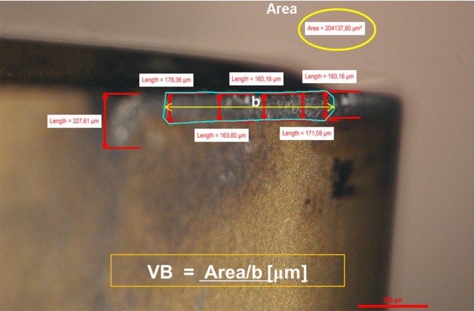

  

  Example for the tool Flank wear detection

In Fig. 10, the VB versus time trends are shown for the investigated conditions.

Fig. 10

Tool Flank wear (VB) versus time for the experimental conditions

The experimental data were used to estimate the function $VB = VB(f,v,t)$, where t represents the tool contact time $t = Y/fv$ (Y is a constant depending on the volume of the material to be removed and other technological parameters, e.g. the depth of cut). The empirical equation found by Linear Regression is:

$$ \begin{aligned} \ln \left( {VB\left( {v,f} \right)} \right) & = 76.6 - 1.763\ln t - 40\ln v - 9.25\ln f \\ & \quad +\, 0.0892\left( {\ln t} \right)^{2} + 5.03\left( {\ln v} \right)^{2} + 0.549\ln v*\ln t + 0.549\ln t*\ln f + 2.095\ln v*\ln f + \theta {\text{ where }}\theta \sim NID\left( {0,\sigma^{2} } \right) \\ & \quad \,\,{\text{and }}\sigma^{2} = 0.02922 \\ \end{aligned} $$

(A1)

Note that the empirical equation is estimated from the experimental data, however we will not use the hat notation because we consider it as if it were perfectly known. This is not an issue because we use the Eq. A1 to sample VB to mimic the real process. Some regression details are reported in the following tables (Tables 6, 7) and the analysis of the residuals is showed in Fig. 11.

Table 6 ANOVA table for regression analysis: Ln VB versus Ln t; LnSpeed; LnFeed

Table 7 Model summary

Fig. 11

Standardized residuals probability (a) and scatter plots (b)

Appendix B: Theoretical optimal conditions

If the Tool wear equation was perfectly known the theoretical optimal solution could be easily derived. Let us consider that the tool wear is a random variate $VB \sim D\left( {\mu \left( {v,f} \right),\sigma_{\varepsilon }^{2} } \right)$ where D is a known probability distribution with ${\text{Expected}}\left( {VB} \right) = \mu \left( {v,f} \right)$ and ${\text{Variance}}\left( {VB} \right) = \sigma_{\varepsilon }^{2}$ The stochastic optimization problem can be transformed into a deterministic one as follows:

$$ \begin{aligned} & \mathop {\hbox{min} }\limits_{v,f} \frac{Y}{v \cdot f} \\ & \Pr \left\{ {VB\left( {v,f} \right) \ge VB_{0} } \right\} \le \alpha \\ & v_{\hbox{min} } \le v \le v_{\hbox{max} } \\ & f_{\hbox{min} } \le f \le f_{\hbox{max} } \\ \end{aligned} $$

(B1)

where VB₀ is the maximum tool wear allowed, in our case it is 0.3 mm. The solution of the problem (B1) is the theoretical optimum $\left( {v_{ott} ,f_{ott} } \right)$, and the corresponding unit optimum tool contact time is equal to $t_{u} = \frac{Y}{{v_{ott} \cdot f_{ott} }}$. The average batch optimal production time can be derived as follows:

$$ t_{opt} = t_{u} B\left( {1 + \alpha } \right) $$

(B2)

Note that Eq. (B2) accounts for the expected proportion of defective parts α (i.e. scraps generated by a tool wear measured at the end of the machining of a feature greater than $VB_{0}$).

Appendix C: Tool wear data

TEST01		TEST_00		TEST_04		TEST05_11
S = 55 m/min F = 0.196 mm/rev		S = 55 m/min F = 0.214 mm/rev		S = 55 m/min F = 0.249 mm/rev		S = 55 m/min F = 0.285 mm/rev
Time	Average VB	Time	Average VB	Time	VB Average	Time	VB Average
(s)	(mm)	(s)	(mm)	(s)	(mm)	(s)	(mm)
10	0.142	10	0.129	10	0.135	10	0.134
30	0.163	20	0.138	20	0.157	20	0.153
50	0.172	30	0.148	30	0.175	30	0.164
70	0.202	40	0.152	40	0.188	40	0.181
90	0.202	50	0.168	50	0.217	50	0.201
110	0.205	60	0.179	60	0.251	60	0.220
130	0.227	70	0.181	70	0.273	70	0.256
150	0.234	80	0.184	75	0.302	80	0.271
170	0.259	90	0.190	80	0.337	85	0.303
190	0.263	100	0.199	85	0.385
210	0.292	110	0.204	90	0.405
230	0.291	120	0.208
250	0.330	130	0.247
		140	0.248
		150	0.273
		160	0.283
		170	0.291
		180	0.301

TEST14		TEST_03		TEST_12		TEST_08
S = 65 m/min F = 0.196 mm/rev		S = 65 m/min F = 0.214 mm/rev		S = 65 m/min F = 0.249 mm/rev		S = 65 m/min F = 0.285 mm/rev
Time	Average VB	Time	VB Average	Time	VB Average	Time	VB Average
(s)	(mm)	(s)	(mm)	(s)	(mm)	(s)	(mm)
10	0.104	10	0.078	10	0.103	10	0.174
20	0.119	20	0.092	20	0.118	20	0.214
30	0.127	30	0.092	30	0.142	30	0.224
40	0.123	40	0.102	40	0.158	40	0.276
50	0.139	50	0.108	50	0.172	45	0.274
60	0.146	60	0.111	60	0.215	50	0.295
70	0.159	70	0.168	70	0.243	55	0.317
80	0.167	80	0.169	80	0.283	60	0.341
90	0.172	90	0.180	90	0.341
100	0.182	100	0.192
110	0.192	110	0.215
120	0.198	120	0.232
130	0.197	130	0.303
140	0.208
150	0.217
160	0.245
170	0.270
180	0.282
190	0.270

TEST09_15		TEST_13		TEST_10		TEST02_07
S = 75 m/min F = 0.196 mm/rev		S = 75 m/min F = 0.214 mm/rev		S = 75 m/min F = 0.249 mm/rev		S = 75 m/min F = 0.285 mm/rev
Time	Average VB	Time	VB Average	Time	VB Average	Time	VB Average
(s)	(mm)	(s)	(mm)	(s)	(mm)	(s)	(mm)
10	0.116	10	0.111	10	0.164	10	0.173
20	0.135	20	0.135	20	0.185	20	0.208
30	0.148	30	0.146	30	0.217	30	0.242
40	0.168	40	0.153	40	0.225	35	0.257
50	0.177	50	0.170	45	0.235	40	0.287
60	0.189	60	0.184	50	0.255	45	0.328
70	0.230	70	0.197	60	0.287	50	0.356
80	0.254	80	0.204	65	0.325
90	0.280	90	0.230	70	0.360
		100	0.239	75	0.456
		110	0.265	80	0.560
		120	0.311
		130	0.412

References

Angün, E., Kleijnen, J., den Hertog, D., & Gürkan, G. (2009). Response surface methodology with stochastic constraints for expensive simulation. Journal of the Operational Research Society,60(6), 735–746.
Box, G. E. P., & Wilson, K. B. (1992). “On the experimental attainment of optimum conditions”. Breakthroughs in statistics (pp. 270–310). New York: Springer.
Costa, A., Celano, G., & Fichera, S. (2011). Optimization of multi-pass turning economies through a hybrid particle swarm optimization technique. International Journal of Advanced Manufacturing Technology,53, 421–433.
D’Addona, D. M., Ullah, A. S., & Matarazzo, D. (2017). Tool-wear prediction and pattern-recognition using artificial neural network and DNA-based computing. Journal of Intelligent Manufacturing,28(6), 1285–1301.
Davim, J. P. (Ed.). (2008). Machining: Fundamentals and recent advances. London: Springer.
Del Castillo, E. (2007). Process optimization: A statistical approach (Vol. 105). New York: Springer.
Devillez, A., Schneider, F., Dominiak, S., Dudzinski, D., & Larrouquere, D. (2007). Cutting forces and wear in dry machining of Inconel 718 with coated carbide tools. Wear,262, 931–942.
Draper, N., & Smith, H. (2005). Applied regression analysis (3rd ed.). New York: Wiley.
Ganesan, H., Mohankumar, G., Ganesan, K., & Ramesh Kumar, K. (2011). Optimization of machining parameters in turning process using genetic algorithm and particle swarm optimization with experimental verification. International Journal of Engineering Science and Technology (IJEST),3(2), 1091–1102.
Kalpakjian, S., & Schmidt, S. R. (2001). Manufacturing engineering and technology (4th ed.). Upper Saddle River: Prentice Hall International.
Klocke, F., Zeis, M., Klink, A., & Veselovac, D. (2012). Technological and economical comparison of roughing strategies via milling, EDM and ECM for titanium- and nickel-based blisks. Procedia CIRP,2, 98–101.
Myers, R. H., Montgomery, D. C., & Anderson-Cook, C. M. (2009). Response surface methodology: Process and product optimization using designed experiments (3rd ed.). New York: Wiley.
Rao, S. S. (2009). Engineering optimization theory and practice. New York: Wiley.
Schorník, V., Zetek, M., & Daňa, M. (2015). The influence of working environment and cutting conditions on milling nickel–based super alloys with carbide tools. Procedia Engineering, 100, 1262–1269.
Taylor, F. W. (1907). On the art of cutting metals. New York: American Society of Mechanical Engineers.
Venkata Rao, R. (2016). Teaching learning based optimization algorithm and its engineering applications. New York: Springer.
Venkata Rao, R., & Pawar, P. J. (2010). Parameter optimization of a multi-pass milling process using non-traditional optimization algorithms. Applied Soft Computing,10, 445–456.
Wang, G., & Cui, Y. (2013). On line tool wear monitoring based on auto associative neural network. Journal of Intelligent Manufacturing,24(6), 1085–1094.
Wang, G., Guo, Z., & Qian, L. (2014). Online incremental learning for tool condition classification using modified fuzzy ARTMAP network. Journal of Intelligent Manufacturing,25(6), 1403–1411.
Yildiz, A. R. (2013). A new hybrid differential evolution algorithm for the selection of optimal machining parameters in milling operations. Applied Soft Computing,13(3), 1561–1566.
Zainal, N., Zain, A. M., Radzi, N. H. M., & Othman, M. R. (2016). Glowworm swarm optimization (GSO) for optimization of machining parameters. Journal of Intelligent Manufacturing,27(4), 797–804.
Zhang, J., Liang, S. Y., Yao, J., Chen, J. M., & Huang, J. L. (2006). Evolutionary optimization of machining processes. Journal of Intelligent Manufacturing,17(2), 203–215.
Zhu, D., Zhang, X., & Ding, H. (2013). Tool wear characteristics in machining of nickel-based superalloys. International Journal of Machine Tools & Manufacture, 64, 60–77.
Acknowledgements
The authors sincerely thank the reviewers for their very helpful comments on earlier drafts of this manuscript, for their time and for their encouragement.
Author information
Authors and Affiliations
Corresponding author
Additional information
Publisher's Note
Springer Nature remains neutral with regard to jurisdictional claims in published maps and institutional affiliations.