
Abstract
We show that the physical principle, “the adjoint associates to each state a ‘test’ for that state”, fully characterises the Hermitian adjoint for pure quantum theory, therefore providing the adjoint with operational meaning beyond its standard mathematical definition. Moreover, we demonstrate that for general process theories, which all admit a diagrammatic representation, this physical principle induces a diagrammatic reflection operation.
1 Introduction
The process theoretic approach [1, 18, 19] provides a novel perspective on the structure of quantum theory by focusing on compositionality. This leads to a diagrammatic representation of quantum processes, simplifying calculations and providing an intuitive way to reason about quantum theory [12, 14]. Furthermore, process-theoretic ideas have been: adopted within other frameworks and corresponding reconstruction theorems [10, 11, 23, 24]; provided a natural setting for theories other than quantum theory [16] which has led to, for example, the study of connections between physical principles and computation [27, 28]; helped solve open problems in quantum computing [7, 22, 25]; and provided a general framework for resource theories [17].
However, one particular diagrammatic ingredient that plays a central role in quantum theory lacks a clear physical interpretation, namely, the diagrammatic counterpart to the Hermitian adjoint. Earlier work has introduced dagger process theories [2, 31] as a generalisation of the adjoint to other theories. However, this is not entirely satisfactory, raising three questions which we answer in this paper.
-
Firstly, why should a theory have have a dagger at all? Section 4 introduces the physically motivated concept of a test structure, associating to each state a test for that state. Section 5 shows that this leads to a dagger.
-
Secondly, why is it always assumed that the dagger should be involutive? Section 5 demonstrates how this is a consequence of the definition of the test structure.
-
Finally, why is the particular dagger of interest in quantum theory the Hermitian adjoint, rather than some other dagger such as the transpose? Section 6 shows that for quantum theory the test structure forces the dagger to be the Hermitian adjoint.
To finish in Sect. 7 we consider process theories with a notion of probabilistic mixing, and show that such theories typically fail to have a test structure. The reason for this is that the notion of ‘testability’ is tightly intertwined with that of ‘purity’. This provides a new perspective on what it means for states to be pure—they are pure if they are ‘testable’.
1.1 Related Work
The physical principle used in this work is closely related to the ‘logical sharpness’ axiom used by Hardy in the generalised probabilistic theory setting [24]. A similar approach to ours was recently suggested by Chiribella [8] who relates the adjoint to time-reversal symmetry. By taking this as an axiom he has shown that the adjoint must be a process theoretic dagger. This however does not uniquely pick out the Hermitian adjoint as a dagger; for example, it also allows for the transpose.
Vicary [32] also characterised the adjoint in process-theoretic terms. However, he required extremely strong assumptions, namely that all dagger-limits exist, which isn’t even the case if one eliminates redundant global phases from quantum theory.
2 Process Theories
A process theory consists of:
-
1.
A collection of ‘systems’, these could represent a physical system such as a photon, but also a mathematical object such as a vector space, or some computational notion such as a data type;
-
2.
A collection of ‘processes’, each of which has an input consisting of a set of systems and another set of systems as an output, these could represent a physical process such as a parametric down converter (this would have a single photon as its input, and a pair of photons as its output), but again, these processes can also be mathematical processes such as a linear transformation, or computational processes such as a sorting algorithm;
-
3.
A composition operation for systems and processes.
This composition operation can be best understood in terms of a diagrammatic notation for systems and processes. In this notation, systems are represented by labelled wires, for example:

Processes are represented as boxes which have a set of input wires at the bottom and a set of output wires at the top. This gives a sense of a ‘direction of time’ as flowing up the page. Dropping system labels for convenience we can denote a process f as, for example:

The shape of this box is irrelevant at this point but the asymmetry will be useful later on.
There are three special types of processes: those with no input, called state preparations (or states for short); those with no outputs, called measurement outcomes (or effects); and those with neither inputs nor outputs, called scalars, which are often taken to be probabilities. Denoted respectively as:

inspired by Dirac-notation [12]. The box around a scalar is often omitted for clarity.
We can now easily define the composition operation of a process theory: given some collection of processes then these can be wired together to form diagrams, which are also processes in the theory. For example:

is a particular wiring together of four processes and must itself be a process in the theory. This composition is subject to the condition that when forming diagrams, any two systems wired together have to be (of) the same (type) and we connect outputs to inputs acyclicaly. Then, essentially, processes in a process theory are closed under forming diagrams.
In order to describe ‘wiring processes together’ explicitly, in particular when the processes are represented by means of standard mathematical models, it is often convenient to consider the following two primitive forms of composition, sequential composition and parallel composition:

which we symbolically denote by \(g\circ f\) and \(h\otimes i\) respectively.
There are also some special scalars for a process theory that are fully characterised by their behaviour under composition. One special scalar is ‘certain’, which is either written as 1 or by the empty diagram, which, of course, when composed with any other process leaves that process invariant:

Another one is ‘impossible’, which is written as 0, and ‘eats’ all other diagrams, in the sense that for each set of input and output wires there is a 0-process, again simply denoted by 0, and when composing any process with the 0-scalar we obtain the corresponding 0-process:

More details on this process-theoretic framework can be found in [18, 19].
Example 1
In the process theory \(\mathbb {C}LM\) the systems are finite dimensional complex vector spaces and the processes are linear maps between these vector spaces. Sequential composition is composition of linear maps and parallel composition is the tensor product. State preparations can be identified with complex vectors, effects with covectors, and scalars with the complex numbers. This ‘mathematical’ process theory will now be used to construct quantum theory as a process theory.
Example 2
We can construct the process theory of pure post-selected quantum processes directly from the process theory \(\mathbb {C}LM\). One way to do so is to consider equivalence classes of linear maps, by ignoring global phases. A more elegant manner of doing the same is by means of doubling, that is, every process is replaced by its double:

where,

represents the conjugate of f, hence obtaining a new process theory \(\mathfrak {D}[\mathbb {C}LM]\) [13]. Composing a state and an effect now gives a positive real number corresponding to the probability of, for example, measuring the effect \(\phi \) given state \(\psi \) according to the Born-rule:

Clearly, processes differing by only a global phase become identical,
Perhaps the most obvious description of \(\mathfrak {D}[\mathbb {C}LM]\) is as a generalisation of ‘Dirac’ notation, when representing states by ket-bras [12].
Remark 1
In category-theoretic terms, process theories can be defined as strict symmetric monoidal categories (SMCs). The systems of the process theory are the objects in the category, the processes are morphisms, and the states for some object are the morphisms from the tensor unit into that object [19, 20].
3 Types of Process Theories
For physical process theories we will always assume that the scalars are the positive real numbers, where the interval [0, 1] corresponds to ‘probabilistic weights’.
Inspired by the physical notion of process tomography, and given the interpretations of states and effects, we can define the following special kind of process theories:
Definition 1
Tomographic process theories are process theories where all processes can be characterised in terms of scalars, see, for example, Eq. 6 in [9]:

Locally tomographic process theories are tomographic process theories which satisfy the stronger condition of ‘local process tomography’ [3, 6, 11, 33]:

Example 3
Quantum theory, in the form of \(\mathfrak {D}[\mathbb {C}LM]\) is a locally tomographic process theory [19, 24].
Previous work on generalising the Hermitian adjoint to the process theoretic setting led to the notion of dagger process theories.
Definition 2
Dagger process theories are process theories which come with a ‘dagger’, \({\dagger _{pt}}\), an operation that assigns to each processes another process as its reflection:

which moreover preserves diagrams, that is, diagrams are reflected ‘as a whole’:

and which, as the notation already suggests, is involutive.
Remark 2
In category-theoretic terms, a dagger process theory is an SMC equipped with a identity-on-objects involutive contravariant monoidal endofunctor [31].
Example 4
Pure quantum theory \(\mathfrak {D}[\mathbb {C}LM]\) involves a dagger structure, namely the Hermitian adjoint. More specifically, for the process theory \(\mathbb {C}LM\) underpinning quantum theory, for a process \(f:X\rightarrow Y\) it is defined by:
by doubling this lifts to \(\mathfrak {D}[\mathbb {C}LM]\).
This raises an important question:
-
Why does it ‘mean’ for quantum theory to have a dagger structure?
and in particular the following two sub-questions:
-
Why does it have to be involutive?
-
Given that there are other candidate dagger structures for quantum theory, most notably the transpose, why is that central role played specifically by the Hermitian adjoint?
4 The New Physical Principle
In what sense can something be considered a state if there is no way to check that it is indeed that state? This suggests the following physical principle:
for each state there exists a corresponding ‘test’.
In the remainder of this paper, after giving formal substance to this principle for general process theories, we will show that the assignment of tests for pure quantum theory is given by the Hermitian adjoint, in doing so we show that for general process theories this principle always gives rise to a dagger.
Definition 3
A test structure, \({\sharp }\), is a mapping from states to effects on the same type subject to the following conditions:
-
1.
Composability of tests:
-
2.
Transformability of tests:

-
3.
Tests produce probabilities:

-
4.
Testability of all states:

-
5.
Sharpness of tests:


Clearly, sharpness constitutes the core of these axioms, the others guaranteeing that test structures are ‘well-behaved’ with respect the interpretation of [0, 1] as probabilities and the structure of process theories. Of course, for pure quantum theory (up to a global phase), there is a unique normalised effect which gives unit probability for a particular normalised state. So it may seem at first like sharpness trivially suffices to single out the Hermitian adjoint (or at least, it’s action on states and effects), however this is not the case, as in quantum theory normalisation of a state itself is defined in terms of the Hermitian adjoint.
Note also that in transformability the use of the notation \({\sharp }\) for arbitrary processes that transform effects is justified, since when we take f to be a state, it can be taken to be the test structure \({\sharp }\).
Remark 3
The above definition is contingent on the assumption that scalars in the theory are positive real numbers with the interval [0, 1] picked out as being ‘physical’ (as these are probabilities). One could generalise the above definition to theories in which the scalars are ordered, with 0 the minimum element and 1 as the order unit.
5 Test Structures Provide Daggers
In this section we show that for general process theories test structures provide daggers, i.e. the reflection operation discussed in Definition 2. Firstly however, we prove some general results regarding test structures, in particular demonstrating that they are involutive which is an essential part of the definition of a dagger and an essential property of the Hermitian adjoint.
Lemma 1
Test structures preserves certainty, \({\sharp }(1)=1\).
Proof
For scalars \(r_1, r_2\) composability implies that \({\sharp }(r_1r_2)={\sharp }(r_1){\sharp }(r_2)\). Let \(r_1=1\) then \({\sharp }(r_2)={\sharp }(1){\sharp }(r_2)\). There are two solutions for this equation, (i) \({\sharp }(r_2)=0\ \forall r_2\) which violates testability leaving just (ii) \({\sharp }(1)=1\). \(\square \)
Lemma 2
Test structures, extended to effects via transformability, are involutive on normalised states, \(\psi ^{{\sharp }^{\sharp }}=\psi \).
Proof
Using transformability and Lemma 1, for normalised states we have,

then, by sharpness, \(\psi ^{{\sharp }^{\sharp }}=\psi \). \(\square \)
Lemma 3
For tomographic process theories, a test structure is involutive on tests for normalised states, \(\psi ^{{\sharp }^{{\sharp }^{\sharp }}}=\psi ^{\sharp }\).
Proof
For \(\psi ^{\sharp }\), a test for a normalised state \(\psi \), we have,

using Lemma 2 for the first equality and transformability twice for the second. Then, by sharpness, \(\psi ^{{\sharp }^{{\sharp }^{\sharp }}}=\psi ^{\sharp }\). \(\square \)
Lemma 4
Test structure preserves probabilities, \({\sharp }(r)=r\).
Proof
Consider,

then tests-produce-probabilities implies that \(0\le p\le 1\) , that is, as the state and the associated test are both physical processes, the resultant scalar should be physical and so be in the unit interval. Now consider,

and again tests-produce-probabilities implies that \(0\le {\sharp }(p) \le 1\), and so, \({\sharp }\) preserves [0, 1]. Now note that Lemmas 2 and 3 imply that,

so the test structure is involutive for [0, 1]. Moreover, composability implies that \({\sharp }\) is multiplicative on all scalars,
The result that \({\sharp }(r)=r\) is an application of standard results regarding functional equations [26]. Multiplicativity and preservation of [0, 1] imply that \({\sharp }(r)=r^a\) where \(a \in \mathbb {R}^+\). Involutivity on [0, 1] demands that \(a=1\) and so \({\sharp }(r)=r\). \(\square \)
Theorem 5
For tomographic process theories, the test structure is involutive.
Proof
Firstly we extend to all states using testability; write an arbitrary state \(\chi = r \psi \) where r is a scalar and \(\psi \) normalised. Then Lemmas 2 and 4 imply that,
Tomography then allows us to extend this to all effects, e,

And finally, using tomography again we can extend this to all processes, f,

\(\square \)
Theorem 6
For test structures of tomographic process theories, the operation \(\sharp \) in transformability can always be chosen in a manner such that it is a dagger.
Proof
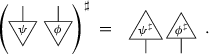
Theorem 5 demonstrates that \({\sharp }\) is involutive, and transformability imposes that if \(f:A\rightarrow B\) then \(f^{\sharp }: B\rightarrow A\), therefore for a test structure to provide a dagger all we need to check is that it preserves diagrams. This is easiest to prove by checking that \({\sharp }\) preserves the two primitive forms of composition, \(\otimes \) and \(\circ \). Consider the action of \({\sharp }\) on the diagram,

there are two ways to apply the composability and transformability axioms to this giving the following constraint,

Next consider applying \({\sharp }\) to the diagram,

here there are again two different ways to apply the transformability axiom, and so we obtain,

The above two conditions (Eqs. 1 and 2) are direct consequences of the test structure axioms and so must be satisfied for the axioms to hold. There is an obvious solution to these:

and so there will always exist an operation satisfying the axioms as well as Eq. 3, and so there is always a test structure which is also a process theoretic dagger. \(\square \)
Theorem 7
All test structures of local tomographic process theories induce daggers.
Proof
The only solution to Eqs. 1 and 2 for a tomographically local theory are Eq. 3 and so \({\sharp }\) must be a dagger. \(\square \)
In the process-theoretic context, daggers have always been taken to be involutive. Now, finally, we have shown that there is a good justification for doing so by demonstrating how this important feature of the Hermitian adjoint follows from the notion of a test structure.
6 Deriving the Hermitian Adjoint for Quantum Theory
In this section we demonstrate that for quantum theory any test structure must be a Hermitian adjoint. In order to do so, we will need to extend the process theory representing quantum theory so that it also includes mixed states, rather than just the pure theory described in the previous sections.
Example 5
We construct the process theory of mixed post-selected quantum processes from the process theories \(\mathfrak {D}[\mathbb {C}LM]\) and \(\mathbb {C}LM\). First note that we have an embedding \(\mathfrak {D}[\mathbb {C}LM]\hookrightarrow \mathbb {C}LM\). This embedding allows us to take sums of arbitrary processes of \(\mathfrak {D}[\mathbb {C}LM]\) within \(\mathbb {C}LM\). These sums, together with the availability of the scalars as processes, allows one to form all linear combinations:

which, in particular, includes all mixtures:

We call the resulting process theory \(\mathfrak {M}[\mathbb {C}LM]\). For notational convenience we denote processes in this theory with bold lines, for example:

We will now assume that transformability applies to \(\mathfrak {M}[\mathbb {C}LM]\), that is:

where now f can now be an arbitrary sum of processes, \(f=\sum _i f_i\). Conceptually, this is a very natural assumption, which states that uncertainty about how a state transforms translates into uncertainty about how the test for that state transforms (see also Sect. 7 below).
Before showing how the test structure provides a Hermitian adjoint we show how another candidate dagger, the transpose, fails to be a test-structure.
Theorem 8
The transpose, T, does not provide a test structure for \(\mathfrak {M}[\mathbb {C}LM]\).
Proof
Consider any states \(\psi \) and \(\phi \) in \(\mathbb {C}LM\) such that \(\mathfrak {D}(\psi )^T\circ \mathfrak {D}(\psi )= 1= \mathfrak {D}(\phi )^T \circ \mathfrak {D}(\phi )\) and, \(\mathfrak {D}(\psi )^T\circ \mathfrak {D}(\phi )=0\) (e.g. the computational basis states). Then \(\mathfrak {D}(\psi + i \phi )^T\circ \mathfrak {D}(\psi +i \phi ) = 1+0+0+i^2= 0\) violating testability. \(\square \)
Theorem 9
The test structure provides a Hermitian adjoint for \(\mathfrak {M}[\mathbb {C}LM]\).
Proof
First note that quantum theory is a locally tomographic additive process theory, and so any test structure provides a dagger. This provides an inner product on the states defined as:

It is simple to check that the inner product axioms are satisfied:
Symmetry:

where the second equality follows by Lemma 4 and the third from the extended form of transformability.
Linearity:

Positivity:

where the second equation uses testability, and similarly positive definiteness follows:
The test structure is therefore the Hermitian adjoint associated to this inner product, defined as \(\langle \cdot ,A\cdot \rangle =\langle A^\dagger \cdot ,\cdot \rangle \). \(\square \)
This explains why the Hermitian adjoint—rather than any other dagger such as the transpose–plays such a prominent role in quantum theory: it has an operational interpretation in terms of a test structure.
7 Test Structures for Additive Theories
Mixed quantum theory \(\mathfrak {M}[\mathbb {C}LM]\) is an example of an additive process theory.
Definition 4
Additive process theories are process theories that come with a notion of ‘sum of diagrams’ that distributes over diagrams:

Remark 4
In category-theoretic terms, additivity of process theories means enrichment in commutative monoids [19]. That the numbers are positive reals means that the morphisms from the tensor unit to itself are the positive reals.
Having both sums and numbers, together with the fact that since numbers have no outputs they can freely move around in diagrams, it also follows that:
Proposition 10
In additive process theories convex combinations (or equivalent, probabilistic mixtures) distribute over diagrams:

where \(\sum _ip_i=1\).
The notion of an additive process theory is similar to the well-studied framework of generalised probabilistic theories [4, 5]. There are many presentations of this framework which are subtly different but in their most recent incarnation they have the structure of an additive process theory [11]. While the usual GPTs have no unique parallel composition operation, the underlying structure of the processes allows one nonetheless to talk about composite systems.
Theorem 11
Additive process theories do not have test structures.
Proof
Consider a state that is a convex mixture of normalised states and assume the existence of a test structure,

where \(\sum _ip_i=1\). Then if we demand that we have a test for that state, \(\psi ^{\sharp }\), then by definition this test must produce probabilities,

which violates sharpness giving a contradiction. \(\square \)
This is not surprising; one cannot deterministically test for a probabilistic mixture of states. However in the previous section we showed that this wasn’t a problem for quantum theory, similarly, Theorem 9 can be extended to additive process theories.
Theorem 12
A process theory with a test structure, embedded within an additive theory, has an inner product defined as:

if we demand that transformability extends to all processes in the additive theory.
Proof
Identical to the quantum case in Theorem 9. \(\square \)
8 Summary and Outlook
In this paper we considered the physical principle of:
for each state there exists a corresponding ‘test’,
in order to gain physical insight into the mathematical structures utilised in quantum theory and more broadly in the process theory framework.
We show that for tomographic process theories this principle leads to a ‘test structure’ which we show provides a process-theoretic dagger. This explains why the dagger should have various properties, involutivity being a particularly surprising consequence. Moreover, for pure quantum theory, we show that the particular dagger provided is the Hermitian adjoint. Therefore explaining why this particular dagger plays such an important role both in the process-theoretic description of quantum theory, and of course, in quantum theory itself in the form of the Hilbert space inner-product.
In the final section we begin to explore the connections between test structures and purity of a theory, showing that theories with mixed states cannot have a test structure. In fact, if we consider process theories that come with a discarding operation—for which we require causality [10, 15]—then we can turn this around and show that a test structure characterises when a process is pure by its testability. Indeed, in forthcoming work [30] we demonstrate that this notion of a test structure, along with a characterisation of pure processes in terms of leaks [21, 29], leads to a reconstruction of quantum theory. The reconstruction is from entirely diagrammatic postulates about quantum processes and quantum-classical interaction, therefore highlighting the primitive role that compositional structures—such as the the test structure defined in this paper—play in quantum theory.
References
Abramsky, S., Coecke, B.: A categorical semantics of quantum protocols. In: Proceedings of the 19th Annual IEEE Symposium on Logic in Computer Science, pp. 415–425. IEEE (2004)
Abramsky, S., Coecke, B.: Abstract physical traces. Theory Appl. Categories 14(6), 111–124 (2005). arXiv:0910.3144
Araki, H.: On a characterization of the state space of quantum mechanics. Commun. Math. Phys. 75(1), 1–24 (1980)
Barnum, H., Wilce, A.: Information processing in convex operational theories. Electron. Notes Theor. Comput. Sci. 270(1), 3–15 (2011)
Barrett, J.: Information processing in generalized probabilistic theories. Phys. Rev. A 75, 032304 (2007)
Bergia, S., Cannata, F., Cornia, A., Livi, R.: On the actual measurability of the density matrix of a decaying system by means of measurements on the decay products. Found. Phys. 10(9), 723–730 (1980)
Boixo, S., Heunen, C.: Entangled and sequential quantum protocols with dephasing. Phys. Rev. Lett. 108, 120402 (2012). arXiv:1108.3569
Chiribella, G.: Teleportation, Time Symmetry, and the Dagger, unpublished
Chiribella, G.: Dilation of states and processes in operational-probabilistic theories. (2014)
Chiribella, G., D’Ariano, G.M., Perinotti, P.: Probabilistic theories with purification. Phys. Rev. A 81(6), 062348 (2010)
Chiribella, G., D’Ariano, G.M., Perinotti, P.: Informational derivation of quantum theory. Phys. Rev. A 84(1), 012311 (2011)
Coecke, B.: Kindergarten quantum mechanics. arXiv:0510032 (2005)
Coecke, B.: De-linearizing linearity: projective quantum axiomatics from strong compact closure. Electron. Notes Theor. Comput. Sci. 170, 49–72 (2007). arXiv:quant-ph/0506134
Coecke, B.: Quantum picturalism. Contemp. Phys. 51, 59–83 (2009). arXiv:0908.1787
Coecke, B.: Terminality implies non-signalling. arXiv:1405.3681 (2014)
Coecke, B., Edwards, B., Spekkens, R.W.: Phase groups and the origin of non-locality for qubits. Electron. Notes Theor. Comput. Sci. 270(2), 15–36 (2011). arXiv:1003.5005
Coecke, B., Fritz, T., Spekkens, R.W.: A mathematical theory of resources. arXiv:1409.5531 (2014)
Coecke, B., Kissinger, A.: Categorical quantum mechanics i: causal quantum processes. arXiv:1510.05468 (2015)
Coecke, B., Kissinger, A.: Picturing Quantum Processes: A First Course in Quantum Theory and Diagrammatic Reasoning. Cambridge University Press, Cambridge (2017)
Coecke, B., Paquette, É.O.: Categories for the practicing physicist. In: Coecke, B. (ed.) New Structures for Physics. Lecture Notes in Physics, pp. 167–271. Springer, New York (2011). arXiv:0905.3010
Coecke, B., Selby, J., Tull, S.: Two roads to classicality. (2017)
Duncan, R., Perdrix, S.: Rewriting measurement-based quantum computations with generalised flow. In: Proceedings of ICALP. Lecture Notes in Computer Science, pp. 285–296. Springer, New York (2010)
Hardy, L.: A formalism-local framework for general probabilistic theories including quantum theory. arxiv:1005.5164 (2010)
Hardy, L.: Reformulating and reconstructing quantum theory. arXiv:1104.2066 (2011)
Horsman, C.: Quantum picturalism for topological cluster-state computing. New J. Phys. 13, 095011 (2011). arXiv:1101.4722
Jung, S.-M.: Multiplicative functional equations. In: Hyers–Ulam–Rassias Stability of Functional Equations in Nonlinear Analysis. Volume 48 of Springer Optimization and Its Applications, pp. 227–251. Springer, New York (2011)
Lee, C.M., Selby, J.H.: Generalised phase kick-back: the structure of computational algorithms from physical principles. New J. Phys. 18(3), 033023 (2016)
Lee, C.M., Selby, J.H.: Higher-order interference doesn’t help in searching for a needle in a haystack. (2016)
Selby, J., Coecke, B.: Leaks: quantum, classical, intermediate and more. Entropy 19(4), 174 (2017)
Selby, J.H., Scandolo, C.M., Coecke, B.: Reconstructing quantum theory from diagrammatic postulates (forthcoming)
Selinger, P.: Dagger compact closed categories and completely positive maps. Electron. Notes Theor. Comput. Sci. 170, 139–163 (2007)
Vicary, J.: Categorical properties of the complex numbers. Electron. Notes Theor. Comput. Sci. 270(2), 163–189 (2011)
Wootters, W.K.: Local accessibility of quantum states. In: Complexity, entropy and the physics of information, pp. 39–46. Avalon publishing, New York (1990)
Author information
Authors and Affiliations
Corresponding author
Rights and permissions
Open Access This article is distributed under the terms of the Creative Commons Attribution 4.0 International License (http://creativecommons.org/licenses/by/4.0/), which permits unrestricted use, distribution, and reproduction in any medium, provided you give appropriate credit to the original author(s) and the source, provide a link to the Creative Commons license, and indicate if changes were made.
About this article

Cite this article
Selby, J.H., Coecke, B. A Diagrammatic Derivation of the Hermitian Adjoint. Found Phys 47, 1191–1207 (2017). https://doi.org/10.1007/s10701-017-0102-7
Received:
Accepted:
Published:
Issue Date:
DOI: https://doi.org/10.1007/s10701-017-0102-7