The Notion of Order in Mathematics and Physics. Similarity, Difference and Indistinguishability

Abstract

The notion of order as a universal and fundamental conceptual category is discussed as being based on sets of similar differences and different similarities. A discussion of relationships between order and disorder is followed by a proposal for a mathematical theory based on non-ordinality which could also have relevance for indistinguishables in physics.

1 Background

The notion of order as a fundamental concept in physical theories was introduced by a series of pioneering papers published by David Bohm [1–5]. These ideas and their relation to quantum phenomena were further developed in discussions with Basil Hiley. A comprehensive survey of these ideas were summarised in their classic book “The Undivided Universe” [7]. For the very latest review of some aspects of this work see the review article by Basil Hiley [6]. The wider relevance of these ideas to philosophy and science will be found in David Bohm’s book “Wholeness and the Implicate Order” [8]. It is important to emphasize that these notions were fundamentally seen as dynamic, so ordering would be the general concept while order is a particular static aspect. Implicate order is thus unfolding into an explicate order and the explicate order enfolding into an implicate order. The verbs unfolding and enfolding are stressing the dynamic nature of order and also how these orders are dynamically related in an overall process.

In [7] (p. 350) Bohm and Hiley write:

“The basic idea is to introduce a new concept of order, which we call the implicate order or the enfolded order. This is to be contrasted with our current concepts of order which are based on the ideas of Descartes who introduced coordinate systems precisely for the purpose of describing and representing order in physical process. The Cartesian grid (extended to curvilinear coordinates), which describes what is essentially a local order, has been the one constant feature of physics in all the fundamental changes that have happened over the past few centuries. In the quantum domain however this order shows its inadequacy, because physical properties cannot be attributed unambiguously to well-defined structures and processes in space-time while remaining within Hilbert space. Thus, for example, the uncertainty principle implies that it is not in general possible to give a definite space-time order to the motion of a particle in its trajectory.”

D. Bohm took order (and structure) as something more universal and fundamental than most of our basic conceptual categories ([3], p.18). Order is concerned with similar differences, arrangements, organisation and structure. In Bohm’s philosophy all these notions are fundamentally dynamic. The ubiquitous character and significance of order is due to the observation that order is common to all that we conceive and perceive which means relating order both to the order of abstract thought of mind as well as to matter and external reality.

Another quotation is clarifying ([7], p. 353):

“Our notions of order in physics have generally been tacit rather that explicit and have been manifested in particular forms which have developed gradually over the centuries in a somewhat fortuitous way. These latter have, in turn, come out of intuitive forms and common experience. For example, there is the order of numbers (which is in correspondence to that of points on a line), the order of successive positions in the motions of objects, various kinds of intensive order such as pressure, temperature, colour etc. Then there are more subtle orders such as the order of language, the order of logic, the order in music, the order of sensation and thought etc. Indeed the notion of order as a whole is not only vast, but it is also probably incapable of complete definition, if only because some kind of order is presupposed in everything we do, including, for example, the very act of defining order. How then can we proceed? The suggestion is that we can proceed as in fact has always been done, by beginning with our common intuitive notions and general experience of order and by letting these develop so as to extend into new domains and fields of application.”

As order is seen to be common to all perception and conception it does not seem possible to give it some exhaustive formal or verbal definition. The question is then how can we hope to describe order? The suggestion implied above is that one could start to make explicit what we already know and point to certain essential features of what is mostly tacit knowledge. The situation has some similarities to bare concepts in formal theories such as class, element and morphism in set theory and category theory. Bohm’s suggestion was that the essence of order is based on organisation of similarities and differences. This proposal was based on an analysis of how we construct and form categories both in perception and in abstract thought.

The formation of categories in perception has been elucidated in numerous both animal and human studies. These experiments suggest that the gathering of differences is the primary data of vision, which are then used to construct similarities. The order of vision starts with the perception of differences and then proceeds by creating similarities of these differences. In abstract thinking there is an analogous process in the formation of categories. Categorization involves two actions: selection (“to gather apart”) and collection (“to gather together”). The act of selection presupposes the perception of differences from some general background. Some of these different “things” are then selected and collected together by regarding their differences as unimportant. Note that their common difference from the background is however important. In order to establish similarity between A and B we are essentially referring to something third making similarity an externally imposed feature. This is brought out more explicitly in three situations, when similarity is established:

• (i) A and B are similar relative a context or background, C. Similarity is established when the exchange of A for B makes no difference in C which can be written as A:C::B:C.

• (ii) A and B are similar in relation to a third entity C. This is commonly expressed as A:B::B:C. The introduction of C gives the possibility of creating similarity.

• (iii) Similarity in a process. Let P denote some process. To be a process something must become different. Consider the process P:A becoming B and B becoming C, where B is different from A and C from B. C could then be similar to A which could represent a process with an aspect of sameness over time.

Thus Bohm proposed that order could be based on organisation of differences and similarities i.e. order is “basically a set of similar differences” ([8], pp. 115–116), which means that differences are insufficient for developing a description of order. In a basic sense similarity and difference are two poles which always go together. However, they are not symmetrical as difference is the most basic of the two. Why? Difference is logically prior to similarity, to establish similarity there must be difference in the first place. Similarity is a consequence of disregarding differences between two things. Furthermore, one could say that difference is an intrinsic feature while similarity is not. To say that A is similar to B only makes sense if we consider A and B relative something different from A and B. As mentioned above, one cannot establish similarity in one step process A→B because if there is no difference, i.e. only similarity, it is not a step. However in B→C, C might be similar to A. This means that in two steps or more there can be some reflexive process in the sense that A refers to C as something similar to A. Having observed that difference is more basic, similarity is still important. They make a pair that always go together. The reason for regarding difference and similarity as a complementary pair is that any concept or category means bringing together different things. This must also apply to the concept “difference”. Difference presupposes similarity in the sense that “differences” are all similar in being different.

2 Order and Mathematics

It was Bohm’s contention that also in mathematics order is more fundamental than relationship and class. For instance, when two things are related they are comprehended within some totality of similar or common order, [3], p. 19. Some order is implicit or explicit always in the background which is logically prior to the notion of relationship or context, apparently implying that order is prior to the notion of relationship. Now the question is: How to develop a mathematics based on order (and structure)? This could entail creating a new set of axioms which treat order and structure as basic concepts. This is customary in mathematics exemplified in axiomatic geometry by point and line as bare concepts. Creating such axioms will no doubt involve a considerable amount of development and refinements of ideas and this goes far beyond the beginnings to be discussed in this paper. The main focus here will be on examples of some simple mathematical order, structures in terms of similarity and difference, and finally a first attempt to formalize a basic aspect of difference expressed as indistinguishability.

2.1 Equivalence Classes

One of the most basic and ubiquitous orders in mathematics is that of an equivalence class, based on an equivalence relation, written as ∼ and defined by:

• 1. a∼a

• 2. a∼b iff b∼a

• 3. a∼b and b∼c implies a∼c

The relation ∼ then defines a class of objects, C, called an equivalence class. We will now look at this in terms of differences and similarities. The main idea behind equivalence classes is to be able to treat objects in the same class as “not different” and to use any such object as a representative for all objects of this class. We are here dealing with two kinds of similarities, itemized as (i) and (ii) in Sect. 1.

• (i) Similarity relative a context, i.e. the equivalence class C. Two objects, a and b, are seen as similar relative C as a and b can be exchanged for each other as representatives of the class C, disregarding all other differences.

• (ii) The similarity between the objects: The equivalence relation ∼ can be seen as denoting a difference between two objects: a∼b. In this sense all objects in a class have similar or the same difference to each other via the relation ∼. By the reflexion condition (1), we have a∼a, so the difference between a and b is the same as the “difference” between a and a. We could express this as a is to b as a is to a or a:b::a:a. Written in this way it becomes explicit that we “cancel” all differences between the objects in the same class.

Furthermore, the equivalence relation ∼ establishes different equivalence classes. These classes can now in turn be treated as differences. It is now possible to establish similar differences between these classes.

2.2 Sequential or Successive Orders Based on Similarity and Difference

Following Bohm’s own presentation and illustration in various contexts ([8], Chap. 5), we first discuss geometrical curves in terms of different orders. The proposal is that (due to D. Bohm) order is based on the organisation of differences and similarities, or somewhat more precise: sets of similar differences and sets of different similarities to be explained below. Orders can further be classified or characterized by two main features; by different classes and by different degrees. Discussing this, I follow D. Bohm’s own examples based on various geometrical curves ([8], pp. 116–117). It should be pointed out that the geometrical curves are assumed to be constituted by different connected chords. Sequential orders can be characterized by two main aspects, accounting for the level of complexity: the class and the degree of an order, which is illustrated by the examples below. Orders of the so called first degree are represented by

• (i) A straight line, being of the first class with one independent difference.

• (ii) A circle, being of the second class with two independent differences.

• (iii) A spiral, being of the third class with three independent differences.

The order of a second degree will be represented by a chain of straight lines, each line of a first class order. Before going into each example it is essential to make some comments: The curves are made up by connected chords where each chord is seen as a set of independent differences. From a suggestion by Arleta Ford [9] similarity denoted by S=(D ₁,D ₂,…,D _n ) relates a set of differences, in this context, different chords. The differences D _i could in turn consist of one, two or more independent differences. The number of these constitutive differences determines the class of the order. When different similarities S ₁,S ₂,… are in question there is the possibility to form a second, or higher, degree of difference. This means that orders of higher degree can be formed. This is because S ₁,S ₂,… are now seen as differences allowing for a new similarity and thus describing order of orders, based on these differences. As indicated, geometrical curves can be analysed as a set of ordered elements: as small intervals of equal length which represent a set of independent differences. Each interval is not only similar to the others in lengths but also different in locations and orientations.

2.3 An Example from Algebra

Before discussing geometrical curves to illustrate various orders, it might be appropriate to give some simple examples from algebra.

A group with the elements a,b and c where a ^m=b ⁿ=c ^p=⋯=e can be seen as having a set of three similarities represented by (S ₁,S ₂,S ₃,…)=(a,b,c,…). Now one could try to relate these different similarities by establishing a second degree similarity. It would now be possible to regard the product ab to represent a difference between a and b and the corresponding difference between b and c would be bc. Similarity thus suggests: ab=bc and it should hold that c=b ⁻¹ ab. This example illustrates a basic feature of structure. Structure is based on orders which have a connection (or link) which “holds the structure together”, [8], p. 119. A group with a ^m=b ⁿ=e where two orders are connected by e, i.e. having a common element. Further examples of structure would be:

• Ex 1 Logic is clearly an ordered structure. If a structure must have connections between orders, this connection is displayed in a proof in logics where the link or connection is established by rules of necessity i.e. necessity directly connects: It gives necessary connection in necessary relationships.

• Ex 2 Quaternions

  Each element i,j and k generates an order of similar differences:

  i,i ²,i ³,…; j,j ²,j ³,…; k,k ²,k ³,… where each i,j and k generates an order which is the constitutive difference of respective order. We have the relations: i ²=j ²=k ²=−1;i⋅j=k etc. which shows that i,j and k are connected by the number −1 i.e. two elements of two different orders turn out to be the same and therefore form a link between different orders. This also shows that the parts are connected to each other in an organized system, structure, via some common element etc.

2.4 Orders of Increasing Degree Represented by Geometrical Curves

2.4.1 Orders of First Degree: A Straight Line

From Fig. 1 we have a:b::b:c::c:d: etc. which constitutes the similarity. This ratio defines a curve of the first class: that is a curve with only one independent constitutive difference denoted as d ₁. The similarity could be denoted S=(a,b,c,…)≡(D ₁,D ₂,…,D _k ) where each difference D _k consists of one constitutive difference in position (d _1(k)).

Fig. 1

A straight line

2.4.2 Orders of the First Degree, Second Class: A Circle

The difference between a and b is both in position and direction. We have two independent differences (d ₁,d ₂). The curve could be said to be of the second class (Fig. 2).

Fig. 2

A part of a circle

We still have a:b::b:c etc. Note that there is only one similarity or ratio, which could be denoted S ¹=(a,b,c,…)≡(D ₁,D ₂,…) and each difference D _k consists of two constitutive differences (d _1(k),d _2(k)) where d _1(k) represents difference of position and d _2(k) represents difference of direction.

2.4.3 Orders of the First Degree, Third Class: A Spiral

In the case of a spiral (see Fig. 3) we get a:b::b:c::c:d:: etc. or i.e. S ¹=(a,b,c,…) with three constitutive differences representing position, length and direction (d _1(k),d _2(k),d _3(k)).

Fig. 3

A spiral

Note that we still have only one similarity as the lengths of the segments are progressively decreasing. However the similarity (or ratio) between successive steps remains invariant. Independence in this context only means that one difference cannot be derived from the other.

2.4.4 Orders of the Second Degree, First Class

To illustrate this, here follows a direct quotation from “Wholeness and the Implicate Order”, [8], p. 116. He writes:

“Thus far we have considered various kinds of similarities in the differences, to obtain curves of the first, second third classes, etc. However, in each curve, similarity (or ratio) between successive steps remains invariant Now we can call attention to curves in which this similarity is different as we go along the curve. In this way, we are led to consider not only similar differences but also different similarities of the differences.”

We can illustrate this notion by means of a curve which is a chain of straight lines in different directions (see Fig. 4). On the first line (ABCD), we can write

The symbol S ¹ stands for “the first kind of similarity”, i.e. in direction along the line (ABCD). Then we write for the lines (EFG) and (HIJ)

where S ² stands for “the similarity of the second kind” and S ³ for “the similarity of the third kind”.

Fig. 4

Straight line segments in different directions

We can now consider the difference of successive similarities (S ¹,S ²,S ³,…) as a second degree of difference. From this, we can develop a second degree of similarity in theses differences. S ¹:S ²::S ²:S ³”, [8], p. 116. This is the beginning of generating a hierarchy of similarities and differences, i.e relating lower levels of order to describe order of orders.

By considering geometrical curves involving differences and similarities of a third, fourth, and so on degree, Bohm introduces the concept of what he calls orders of higher degree.

Each straight line in this illustration is as in the case of a straight line represented by one independent difference:

Bohm now takes the similarities (S ¹,S ²,S ³,…) and constructs from these new differences between successive similarities S ¹,S ²,… , which form a new set of differences, which are denoted differences of a second degree. It is then possible to relate these differences to get a second degree of similarity. A. Ford has suggested a simplification, [9]: Instead of considering the difference between the successive similarities (S ₁,S ₂,S ₃) as a second degree of difference it is expedient to take the very similarities (of a first degree) as the differences of a second degree. The very idea of order of higher degree implies that the similarities (of a first degree) are different, and as they are different it is natural to regard them directly as differences of a second degree. This facilitates both a symbolization and an algebraic approach for the notation and development of multi-level orders.

D. Bohm’s own view of the relationship between order and mathematics was essentially that the current aspects of order in mathematics were insufficient. So for instance, the order relation < tacitly presupposes that each element is considered as completely constituted, i.e. the order of elements is external to the elements themselves, referring to how the elements are different from each other and then being related. This is thus contrasted by the above discussion where the order of differences of the chords, etc actually was seen as constituting the curve, not only describing it. The more general challenge as Bohm saw it was ([3], pp. 23–24):

To develop a new structure of mathematical symbolism that takes into account:

• The hierarchical potentialities of order.

• Not assuming that a mathematical structure is composed of separate elements where orders and relationships are external to what these “elements” are.

• Explicitly differentiate between constitutive and descriptive order/difference. To be able to exhibit how these orders are related in a vast set of cross-references of one aspect of structure to another.

3 Order–Disorder

The notion of absolute disorder is a non-category. Some kind of order is common to everything we can perceive and conceive. There is also a general problem in defining a fundamental concept (like disorder) only by negation. The reason is that the core meaning of a definition is to keep something within certain limits. This is not equivalent to a definition by negation as this means going outside these limits. It is not a problem when the definition is made in a limited context. But universal and basic concepts are not in a limited field and a negation will be without limits: saying disorder is everything which order (which notion itself cannot be exhaustively defined) is not which makes it unclear what is being referred to, [4], p. 308. Furthermore, to define absolute lawlessness and featurelessness or disorder positively as well as negatively we will inevitable refer to some kind or order, rule, law, feature etc. which leads to the absurd concept of law of lawlessness, feature of featurelessness etc. which makes it contradictory. Instead we can talk about relative disorder, relative non-regularity etc. We are free to talk about order of an indefinitely high degree, or of infinite degree. Instead of equating randomness with absolute disorder, we can approach this concept differently by referring to orders of infinite degree. Disorder in the “absolute sense” can be exchanged with an order of infinite degree, from which we in principle could abstract any suborder or particular order, [11], pp. 137–141.

3.1 Related Orders: Causality–Determinism

When two orders are related and when given one, we can more or less determine the other. This has been a necessary condition for prediction and causality in science. Prediction is based on the relation between the order of physical events and the order of time. Long before modern science, astronomers were able to relate the positions of planets, moon etc with the clock-time order and from this the time order make predictions of future positions. Determinism and causality are based on the fact that two orders determine each other. In physics determinism as predictability is based on a close relationship between the sequential order of time and an order of physical events. Seen in the general context of order, predictability is then a particular relationship between the order of time and events, where a few steps in time determine the whole order of events. The concept of implicate order as proposed by Bohm can be regarded as such an example where a basic order of physical processes is not related to time-order but to an order of transformations of an algebra, denoted as an order of enfoldment.

3.2 Unrelated Order: Relative Disorder and Randomness

A classical example of a random series based on physical events is the flipping of coins. The relevant two orders are: The succession in time of throws and the outcomes. These two orders are almost independent which means that given the time-order, one cannot determine the throws and given the throws one cannot determine the time-order. This is what is called a random sequence. This does not mean complete disorder relative time order because the outcomes are not irregular in respect to initial conditions, of position and velocity of the coin. Even if given a series of random events with no known law like dependence on anything else, two such series would be distinguished from one another. In this elementary sense they have some order. The point is that total lack of order has no real meaning.

3.2.1 Unrelated Orders

In statistical physics, thermodynamics, the movements of the individual particles depend on a very large number of other particles. There is almost a complete unrelatedness between the individual particles, the micro order. This independence is a necessary condition for the application of probability theory which in turn gives rise to a statistical relationship, or a macro order which is expressed by laws like pV=nRT which represents a large scale order relating pressure, volume and temperature of a gas. This order is of a much lower degree than the microscopic order of movements of independent molecules and almost insensitive to the order of the microscopic level and where the order of time has disappeared completely. This illustrates that in the limit of large numbers, random orders can approximate regular and simple orders of low degree. In the given example the gas law does not even make sense at the microscopic level. Another example related to physics is Brownian motion. This case illustrates that the independence of the micro order and the macro order is only relative. A small particle is exposed to random collisions. The statistical analysis (random walk) gives that the distance from some original position is proportional to the time passed times the square root of time: $\mathit{constant}\cdot\sqrt{t}$. This means that we have not lost a relation to time-order completely and we can use this statistical relation for predictions. Therefore this example displays a situation somewhere in between complete loss of a relationship between a microscopic order, appearing in the dynamics of the particles, and macroscopic order.

3.2.2 Disorder and Randomness; Context Dependence

Relative disorder is not only to be found in physical events. As a simple illustration, take the square root of 2. Express $\sqrt{2}$ as a string of symbols, representing the digits in some base. If now part of this string is presented to someone who does not know its origin, the person would find it fulfilling all criteria of randomness and “lack of order”, and as a consequence could in no way predict the next digit from the previous ones. In the context, when the appropriate algorithm is given, it is perfectly determined. So we have clearly a context dependence of randomness.

An analogous situation is the generation of random numbers by a computer. In a context that does not include the computer and the algorithm, the number series produced will clearly exhibit randomness. Again in a context including the program the numbers are generated by an algorithm of a quite low degree of order. The two notions order and disorder have been seen to be not mutually exclusive but rather complementary. Science is in fact exploring new orders between chaos and simple kinds of order as is seen in turbulence, chaos theory, fractals etc. Prigogine has demonstrated that regular orders can emerge in certain chaotic systems. This means that these systems must move through a whole spectrum of orders between chaos and regular orders of quite low degree. Furthermore, Mandelbrot has shown the existence of set with fractal dimensions, between spatial dimensions. Such sets can be of almost infinite complexity of almost infinite degree of orders as exemplified by Julia sets. This situation is also reflected in modern chaos theory. Incorporating order as a fundamental category in our thinking could give new perspectives to perceive and conceive new laws and regularities in Nature.

3.3 Indistinguishables: Different but not Distinct

We have now been discussing mainly sequential orders. What could be said about non-sequential orders? The most basic sequential order is based on differences which can be ordered or indexed, i.e. having ordinality in a mathematical or set theoretic sense. This way of thinking leads rather directly to a notion of non-ordinality or indistinguishability.

The motivation behind studying indistinguishables is here three-fold. As mentioned earlier D. Bohm suggested that order is basically described as a set of similar differences and different similarities. Difference is seen as more basic than similarity. The reason is that similarity presupposes difference which makes difference logically prior to similarity. In fact, similarity is a consequence of disregarding difference. In such a context difference becomes fundamental. It is therefore natural to ask if there are different kinds of basic differences, i.e. is there really only one difference, usually expressed as in a≠b? It is conceivable that two different objects comprise of two aspects of difference: one collective and one individual. The collective aspect refers to some collective totality, whereby different objects are different because they are differently contributing to the whole, or collective. One could say that each object is defined collectively by being different from all others in the shared context or collective. The individual difference then concerns a direct relation between two individuals. This difference is always used when some object is named, labelled, indexed to identify each object uniquely. A “collective” difference is then reflecting that objects are different in the sense that they, by the very being part of some whole or collection, are differently contributing to this whole. If they were not, they would not be different at all. If cardinality represents the collective aspect of difference, ordinality would represent the individual. It is hard to see any reason why these two aspects necessarily should be identical. This motivates a proposal of two basic kinds of differences where non-ordinality will imply indistinguishability. Another reason for a discussion of indistinguishables is that there are very few systematic attempts to deal with id:s (here after I use the shorthand id for indistinguishable). Indirectly, any limitation in the scope of the subtlety of mathematics could entail limitations in aspects of our understanding of reality. Thirdly an obvious example of collective difference but not of individual difference comes from physics. In quantum theory we have the notion of Bose-Einstein statistics describing bosons, which are treated as indistinguishables. Moreover Fermi-Dirac statistics deals with indistinguishable fermions. Even in “classical” physics the notion of id turns up in discussions of Gibbs paradox in the context of statistical thermodynamics. There is no basic mathematical treatment available in these situations but rather general rules of thumb.

What would a theory based on non-ordinality but only on cardinality look like? There is something reminding of this, namely multisets, where elements are allowed to repeat in a class, thus being identical, but still contributing to the cardinality. Examples are found in combinatorics; in repeated roots of polynomials, multisets or prime factors etc. However, multiset theory does not really treat non-ordinality but rather only multiple occurrences of identicals. Instead I like to explore a possible framework of a theory based on objects which are different but lacking ordinality. This suggests:

• (i) The introduction of a third pairity relation between objects (to differ from multiset theory), denoted as α⊻β.

• (ii) Relaxing ordinality, necessarily implies that such objects cannot be individually labelled, named or indexed.

• (iii) Taking the “collective” aspect of difference, as fundamental. This means that the objects are differently contributing to the cardinality of a class, but not to the ordinality. Differently put: Each object contributes to the whole by contributing (differently) to the cardinality of some class where the class represents a “whole”.

The original source of inspiration was Parker-Rhodes work on id:s in [10]. Many ideas and notions in this discussion derive from this work. However, the path taken here is not faithful to that theory being triparitous at a semantic level, which builds on a non-transparent notion of information.

[Some notations: In α⊻β, α and β are called id:s. A class containing id:s is called a Sort denoted as S. To avoid confusion with Set-theory “β in S” means β belongs to S.]

4 A Novel Parity Relation ⊻, Representing a New Difference Between Objects Which Lack Ordinality

4.1 Preliminaries

A theory of id:s is a theory about a novel category of items, which entails a new kind of difference between them. This kind of difference reflects a “collective” difference, where such objects cannot be ordered in any unique way, or cannot individually be contrasted to each other by some unique indexing or labelling procedure. On the other hand we want each object to contribute differently to some totality or more precisely here, to a cardinality. To deal (more systematically) with this situation a novel parity relation, denoted as α⊻β, between id:s is introduced. This difference can naively be said to lay “in between” identity and ordinary distinction (here written as ⊥). Thus we arrive at six parity relations based on =, ⊻ and ⊥ (Table 1).

Table 1 Parity relations

All relations are symmetrical. It should be emphasized that while being triparitous a theory of id:s is fundamentally different from a many-value logic on one hand and from a theory of multisets (allowing for a number of identical elements in a set) on the other. This will become more clear below. Each negation of =, ⊻ and ⊥ is defined as the disjunction of the other two. This is important to stress as, for instance a † b could mean that neither =, nor ⊻ can be excluded.

Below follows an outline of a theory of a (quasi) class of indistinguishables (id:s). It should be pointed out that a formal Sort-theory is still under construction and the axioms below can be subjected to modifications at a later stage. These (quasi) classes are called Sorts and have members and parts that might be id:s. Parenthesis are used to denote contexts, such as $[\mathcal{A}]$ which can be read as “in the context of $\mathcal{A}$”. A “collection” is a specific context, written as (A) and provides to some extent an analogy to {M} in set theory. A collection, (X), has the main function of “enclosing” which is inside, entailing a separation from what is outside, thus creating a collective context or a whole. A part of a Sort is called subsort or member.

Definition 4.1

(Sort)

• (i) A Sort is a (quasi) class of objects which might contain id:s.

• (ii) A Sort is called pure iff a ⊥ b does not hold for any two objects in the Sort. Otherwise it is named mixed.

Axiom 4.1

(Existence of Sorts)

∃x, ∃y and ∃S (Sort) such that x in S & y in S, where x⊻y.

Axiom 4.2

(Axiom of cardinality)

Every Sort is associated with a unique cardinal number, which is identical to a natural number.

Axiom 4.3

(Pairity relations of Sorts)

• 1. Two Sorts, or their parts or members, must have one of the possible six pairity relations.

• 2. S and T two Sorts: if there is no object α in S and β in T such that α⊥β and if S and T have equal cardinality, either S=T or S⊻T.

Comment: If for some α in S and some β in T α⊥β, this will imply that S and T can be indexed by α and β respectively and can thus be ordered, hence S⊥T.

Axiom 4.4

(Axiom of extensionality)

(∀z;z in S⇔z in T)⇔S=T. S is equal to T iff any item in T is an item in S and vice versa.

Axiom 4.5

(Collection Axiom)

For any χ, the collection of χ, denoted (χ), defines a whole comprising the same objects as in χ, while

• (i) χ≠(χ), except when  cardχ=1 or  cardχ=0.

• (ii)  cardχ= card(χ), unless χ itself a collection.

• (iii) ((χ))=(((χ))).

• (iv) Given x in A, and some y in (A) it is generally undecidable whether x=y or x⊻y, without further information.

Axiom 4.6

(Identity Axiom)

χχ=χ (i) and χ=ψ iff  cardχψ=1 (ii).

Definition 4.2

(Empty Sort)

An empty Sort ∅, for any x ⇒x not in ∅.

Definition 4.3

(Singleton)

A singleton is a Sort, s, for which there is only one object in s: x in s and y in s⇒x=y.

Axiom 4.7

(Existence of singletons)

There exists singletons according to Definition 4.3 such that

• (i)  cards= card(s)=1.

• (ii) s=(s).

Comment: The second criteria makes Sort-theory very different from set theory where members and sets are clearly separated, M≠{M}.

Axiom 4.8

(Existence of Empty Sort)

There exists an empty Sort denoted ∅ according to the Definition 4.2 such that  card∅=0 and it holds that: ∅=( ) and (∅)=( ).

Comment: The uniqueness of ∅ follows from Axiom 4.4 (axiom of extensionality) by assuming ∅₁ and ∅₂ and observing ∅₁≠∅₂ cannot be falsified.

Postulate 4.1

An element or set in the category of Set can only have the parity relation ⊥ (distinction) with an object in a pure Sort.

Postulate 4.2

Given aRb and bRc where R is one of the parity relations R∈{=,⊻,†}. It can never be the case that any pair of a,b,c is distinct (such as a⊥c).

Postulate 4.3

Given aRb and b⊥c where R∈{=,⊻,†} implies distinction between a and c, i.e. a⊥c.

Postulate 4.4

(Invariance to permutation of id:s)

In any relation or expression where two id:s are permuted or interchanged, provided that there is no ambiguity that the same token, say x, or y refer to the same object, for every occurrence of the same, the relation or the expression remains invariant.

Comment: “Postulate” reflects a more temporary status than “Axiom”.

4.1.1 Id:s Form Equivalence Classes of Sorts

From the transitivity implied by Postulate 4.2 it is seen that the pairity relation a†b is an equivalence relation. It holds that: a†a (as † is the disjunction of ⊻ and =) and also: a†b and b†c⇒a†c as a⊥c is impossible due to Postulate 4.2. The term “class” is not used in a set-theoretic way. Moreover a in E ₁ and b in E ₂ where E ₁ and E ₂ are two different sort-classes of id:s. The only possible relation is a⊥b as otherwise a and b would be related by = or ⊻, i.e. they would be equivalent.

Definition 4.4

The equivalence sort-classes of id:s define pure Sorts.

4.2 Introduction of “Ordered” Pairs; Non-Ordinality

The basic ordering of two objects is commonly defined as an ordered pair P(a,b)=(a,(a,b)). The parenthesis ( ) denote a collection of items as defined above i.e. a Sort seen as a collective whole. To be consistent with a notion of non-ordinality as formulated in the axiom above, the natural choice is P(a,b)=P(b,a).

Axiom 4.9

(Non-Ordinality)

P(a,b)=(a,(a,b))=(b,(a,b))=P(b,a).

4.2.1 Fundamental Ambiguity

Consider P(a,b)=P(b,a) written as (a,(a,b))=(b,(a,b)). If the first objects a and b in respective pairs would be well defined it would imply a=b. To avoid this an alternative is to say that the first object is not well defined. The proposal here is that the first element only represents one of the two elements in (a,b), and does not refer to a particular one. To be consistent with this approach it is further assumed that in expressions like ((a,b),(a,b,c)) we can only say that the first “collection” of objects appears in the second (a,b,c) and cannot make a difference between this expression and the expressions ((a,c),(a,b,c)) or ((b,c),(a,b,c)). To deal with this kind of ambiguity a special quantifier $\hat{U}$ is called for: $\hat {U} \ a \ b \ c$ , meaning one of a,b,c but no one in particular. This will be discussed separately below.

4.2.2 Context Dependence

The ambiguity caused by the non-ordinality axiom P(a,b)=P(b,a) (Axiom 4.9) means that in general one cannot demonstrate that two identical symbols refer to the same object like the two symbols a in P(a,b)=(a,(a,b)) appear in different contexts. When the contexts are different there is no guarantee that we can unambiguously refer to the same item or object. To have a consistent theory, this is then generalized: Given some collection (α,β,γ) of id:s. If now one or more are duplicated or “taken out” of the collection these symbols cannot unambiguously refer to the same objects as being in the original collection. To bring this out more explicitly: Consider the “collection” C of unordered pairs: C=((x,z),(y,w)). Now permute x↔y giving C′=((y,z),(x,w)) which by the Postulate 4.4 leaves C unchanged that is: C=C′. If we now try to identify say x and z in both C and C′ i.e. set x=z in both C and C′. We would get ((x,x),(y,w)) for C, and as (x,x)=(x), according to the identity axiom (Axiom 4.6), we have the equality: ((x),(y,w))=((x,y),(x,w)) (for C′), which obviously is false. The mistake is to identify two elements x,z being in different contexts or collections and having different pairity relations in C: x⊻z while in C′: x†z. This is because x and z are in different contexts in C′, i.e. the contexts of (x,w) and (y,z) respectively. Without further information it could be that x=z and hence we can only say x†z. This kind of context dependence calls for particular rules when we can relate two id:s.

4.3 Existential and Universal Quantification

4.3.1 Existential Quantification

In a standard approach existential quantification of a predicate is generally expressed as ∃x; Q x is true, where x belongs to some class C and asserts that there are some members in C which have the property Q. It is assumed that it is possible to select the appropriate items by some (unspecified) procedure. However, in the case of Sorts, the nature of id:s does not allow for selecting a particular item as this would imply some labelling, naming or indexing. Even to say that some particular item in a Sort has the property Q is to assert something that cannot be proven by any algorithmic approach. By testing one by one we cannot identify if one item has been tested or not. To assert that some member of a Sort has the property Q is something that cannot be disproven. If we test some x in a Sort to see if Q x is true and find that it is not, we have to go on testing every member in S. However, we cannot label which ones have been tested so we could end up in indefinitely examining the same individual. There is however one exception. In a definition one could demand that something having a property Q shall exist. Such a statement is not open to test. However, it may turn out in some other context that the definiend is proven not to exist if due care is not taken. Generally this is avoided by explicitly only taking the cardinality of the individuals having property Q. More precisely: as any Sort has a unique cardinal number one should be able to assert that in a given Sort a certain subsort with definite cardinality has the property Q x, as the subsort is only specified up to cardinality.

4.3.2 Universal Quantification

The situation is different regarding universal quantification i.e. using all, every or any. As no particular selection is involved, universal quantification does not create problems. We can write this as: ∀x; x in C⇒P x=( ) where C some (Sort) class. No testing procedure is required in universal quantification: we can arbitrarily pick any one.

4.3.3 Conditional Quantification

From the observation that we can consistently deal with universal quantification, it can be argued for a limited form of quantification

$$\forall x;\quad Q\ x=(\ )\quad \Rightarrow\quad P\ x=(\ ) $$

where accordingly P x is true for anything that holds for Q x. That Q x is true could be the result of some definition or else unproblematically given.

4.3.4 Negation of Universal and Conditional Quantification

The negation of a universal quantification: ¬(∀x;x in C⇒P x=( )) “destroys” the universal quantifier ∀ as it means that there are some x in C for which P x is false, or (not P) is true, turning the statement into an existential quantification. This does not mean that we cannot negate P, but we have to use some conditional quantification ∀x;Q x=( )⇒(not P)=(/), which says that P does not hold for any x such that Q x is true. This discussion is now expressed in the following axioms.

Axiom 4.10

(Forbidden existential quantification)

Unconditional existential quantification is forbidden, except when demanded so by (reasonable) definitions. Reasonable should be read as non-inconsistent or non-incoherent.

Moving on to the negation of conditional quantification to consider ¬(∀x; Q x⇒P x). This means that there exists some x for which Q x is true, but P x is false i.e. (∃x; P x=(/) and Q x=( )). This is existential quantification and forbidden. This does not mean that “not P” (¬P) is meaningless. We can say that ¬P does not hold for any x such that Q x is true. As “any x” is universal quantification it is allowed for and we write ∀x; Q x=( )⇒¬P x=(/).

Axiom 4.11

Universal quantification is allowed for.

Axiom 4.12

Conditional existential quantification is generally allowed for: P holds for any x such that Q x is true.

Axiom 4.13

(Existential quantification involving cardinality)

∃x in S;  card(x in Sforwhich P x istrue)=n, n∈N and n ≤ card S.

This defines a subsort h of S: $\forall x \ \mathrm{in}\ h \Rightarrow P \ x \mathrm{\ and\ card}(h)=n$.

5 Subsorts, Unions and Other Things

A subsort of a Sort a part of S which is defined as usual:

Definition 5.1

(Subsort)

h⊆S⇔∀x(x in h⇒x in S) and  cardh≤ cardS.

Definition 5.2

(Proper subsort)

$\exists x \ \mathrm{in}\ S\mbox{ and $x$ not in }h$ and  cardh< cardS. (Due to the existential quantifier ∃ we demand the existence by definition.)

Some comments:

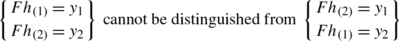
• 1. Writing x in h, y not in h says that only one of two elements x,y,((x,y) in S), one belongs to h, the other does not. It is not meaningful to assign a certain property to x in particular (in this case “x in h”) as this would entail a “labelling” of x and y which is forbidden. Consequently x in h,y not in h cannot meaningfully be distinguished from y in h,x not in h.

• 2.  cardh ₁≠ cardh ₂⇒h ₁⊥h ₂; (see Axiom 4.3); The reason is that h ₁ and h ₂ can be assigned two different unique cardinal numbers.

• 3.  cardh ₁= cardh ₂ gives without further information the pairity relation h ₁†h ₂ as h ₁ and h ₂ have equal cardinality. If they are known not to be identical we will get h ₁⊻h ₂.

• 4. Given a Sort S,  cardS=N each n<N will entail an equivalence (Sort) class of subsorts each with cardinality n. It is seen from this that we get N distinct classes of subsorts of S, one for each cardinality.

As cardinality is fundamental we state:

Theorem 5.1

Given a subsort h of a (pure)  SortS, h⊆S it holds that:  cardh= cardS⇔h=S.

Proof

(⇒): From Axiom 4.3  cardS= cardh⇒h⊻S or h=S. If h⊻S we can permute h and S in h⊆S i.e. S⊆h and according to Axiom 4.4 it follows h=S. The implication in the other direction is immediate. □

5.1 Relative Complement

Given h, a subsort in S we need to construct the complement of h in S. We do this by the following

Definition 5.3

(Relative Complement in S)

Every h in S defines a subsort Ch in S

• (i)  cardh+ cardCh= cardS.

• (ii) ∀x in S it holds that x in h or x in Ch.

• (iii) From (ii) follows immediately that C[Ch]=h. Consider Ch and C[Ch] where every x either in Ch or C[Ch], so if x not in Ch⇒x in C[Ch]. While (ii) gives also x in h. If x in h⇒x not in Ch and thus x in C[Ch] which gives the equality (Axiom of extensionality).

5.2 Intersection of Sorts

Definition 5.4

(Intersection of Sorts)

The intersection of S ₁ and S ₂: S ₁∩S ₂⇔x in S ₁ and x in S ₂.

5.3 The Union of Sorts

Considering the usual definition:

Postulate 5.1

• (i) x in S ₁∪S ₂⇔x in S ₁ or x in S ₂. This reveals a difficulty: If we want to identify the members in S ₁∪S ₂ there is no clear way to associate an element x uniquely with S ₁ and not with S ₂. This would imply a labelling of the elements: say x in S ₁, x not in S ₂ while y not in S ₁, y in S ₂. This is indistinguishable from x in S ₂, x not in S ₁ and y in S ₁, y not in S ₂. Therefore (i) calls for a modification: It is clear that S ₁∩S ₂ and  cardS ₁∩S ₂ does not create the same problem because every element x in S ₁∩S ₂ has the same “label” namely “x in S ₁ and x in S ₂ ” or is indexed by  cardS ₁∩S ₂. Using intersection and relative complement, union can be expressed and defined by: S ₁∪S ₂=C[CS ₁∩CS ₂] where S ₁ and S ₂ belong to the same equivalence class (Sort), and CS _i denotes the complement of S _i in S.

• (ii) S ₁∪S ₂=C[CS ₁∩CS ₂].

• (iii)  cardS ₁∪S ₂= cardS ₁+ cardS ₂− cardS ₁∩S ₂.

Now, take the complement of each side of (ii): CS ₁∪S ₂=CS ₁∩CS ₂, as CCS=S. For any x in S ₁⇒x not in CS ₁⇒x not in CS ₁∩CS ₂⇒x not in CS ₁∪S ₂⇒x in S ₁∪S ₂ and analogously for x in S ₂. This demonstrates that we can work comfortably with the usual definitions of union under the restrictions given. This also gives S _i ⊆S ₁∪S ₂, (i=1,2).

Theorem 5.2

 cardS ₁∩S ₂= cardS ₁ if and only if S ₁⊆S ₂

(⇒):  cardS ₁∪S ₂= cardS ₁+ cardS ₂− cardS ₁∩S ₂= cardS ₂. Assume the contrary: ∃x;x in S ₁ and x not in S ₂ implying  cardx∩S ₂=0. x in S ₁⇒x in S ₁∪S ₂ as well as x∪S ₂⊆S ₁∪S ₂ (by definition of union). Hence,  cardx∪S ₂≤  cardS ₁∪S ₂, as x∪S ₂ is a subsort of S ₁∪S ₂. But then  cardx+ cardS ₂− cardx∩S ₂≤ cardS ₁∪S ₂ i.e. 1+ cardS ₂≤ cardS ₂ which is a contradiction ⇒ for all x in S ₁ it holds that x is in S ₂.

(⇐): x in S ₁⇒x in S ₂⇒x in S ₁∩S ₂⇒S ₁⊆S ₁∩S ₂⇒ cardS ₁≤ cardS ₁∩S ₂ and obviously:  cardS ₁∩S ₂≤ cardS ₁ which implies  cardS ₁= cardS ₁∩S ₂. The theorem gives immediately that  cardS ₁∩S ₂= cardS ₁= cardS ₂⇔S ₁=S ₂.

5.4 Partitioning of a Sort

Definition 5.5

A partitioning of Sort S is a class H of subsorts and is denoted as H=|h ₍₁₎,h ₍₂₎,…,h _(k)| where

• (i) x in h, h subsort of H⇒x in S.

• (ii) Any two subsorts h′,h″ of H⇒h′∩h″=∅. (∅ is here the empty sort.)

• (iii)  cardh ₍₁₎+ cardh ₍₂₎+⋯+ cardh _(k)= cardS.

These conditions imply

• 1. h′, h″ subsorts of H:  cardh′∩h″= card∅=0.

• 2. S=⋃h _(k).

As every h _(k) in ⋃h _(k) and as h _k is a subsort of S this implies that ⋃h _(k) in S.

Furthermore,

(1)

From Axiom of cardinal extensionality it follows that ⋃h _(i)=S. Note that the partition defines a multiset { cardh ₍₁₎,…, cardh _(k)}. We need further to postulate the existence of partitioning.

Postulate 5.2

(Partition postulate)

Given any Sort, S with  cardS=N. For every integer partitioning of N={n _i }, there is a corresponding partitioning of S into subsorts h _(i), where  cardh _(i)=n _i such that S=⋃h _(i) and h _(i)∩h _(j)=∅ for h _(i)≠h _(j).

As has been observed before, such a partitioning is only unique up to cardinality, any permutation of id:s between the subsorts leaves the partitioning invariant.

6 Blur: A Novel Ambiguity Quantifier

No property of id:s is more basic than being subject to confusion. As was seen from discussing “ordered pairs” one would need some consistent notation to deal with situations like P(a,b)=(a,(a,b))=P(b,a)=(b,(a,b)), where the first element does not refer to a particular element in (a,b) but to one of the two elements. Given (a,(a,b)) we want to express something that represents one of (a,b), but indecisive which, and consequently not the two taken together as a collective. This is written as $P(a,b)=(\hat{U} \ a \ b,(a,b))$ where $\hat{U} \ a \ b$ denotes and represents one of (a,b) but not one particular. If we exclude distinction, a⊥b, the only possible pairity relation between $\hat{U} \ a \ b$ and the elements a,b could be: $a \dag\hat {U} \ a \ b$ and $b \dag\hat{U} \ a \ b$. To restrict $\hat{U} \ a \ b$ to the collection (a,b) we would also need to say that $\mathrm{card}(a,b,\hat{U} \ a \ b)=2$. We will now formulate a definition of $\hat{U}$.

Definition 6.1

(Blur $\hat{U}$)

The blur of two entities, x and y, denoted as $\hat{U}xy$ yields undecidably either x or y but not both together. Two necessary conditions must be fulfilled: For any predicate or property P it holds that:

• 1. $P\ \hat{U}xy\Rightarrow Px$ and Py.

• 2. Px and $Py\Rightarrow P\ \hat{U}xy$.

$\hat{U}xy$ is then generalized in the obvious way to several entities $\hat{U}xyz\cdots\,$. The notion $\mathop{\hat{U}}_{n} h$ can be used for the blur of n elements in some subsort h. From 2, when x and y also are singletons with cardinality one we have:  cardx=1 and  cardy⇒ $\mathop{\mathrm{card}}\hat{U}xy=1$. (Here card is substituted for P.)

6.1 Some Relations Involving Blur

Definition 6.2

$\hat{U} \hat{U} = \hat{U}$.

For a union $z\ \mathrm{in}\ \hat{U}h \cup\hat{U}g$ could be written ¬(z not in h∨z not in g)=¬(z not in h∪g).

Definition 6.3

$\hat{U}h \cup\hat{U}g = \hat{U} h\cup g;\hat{U}h \cap\hat {U}g=\hat{U}h\cap g$.

As an illustration we evaluate $\hat{U} | \hat{U}h \cup\hat{U}g |$: from the Definition 6.3 $\hat{U}|\hat{U}h \cup\hat{U} g|=\hat {U}|\hat{U} h\cup g|=\hat{U}\hat{U}h\cup g=(\mbox{by Definition~\protect{6.2}})=\hat{U}h\cup g$. Applying associativity gives $\hat{U}a \hat {U}ab = \hat{U} \hat{U}aab = \hat{U}ab$ which also is easily generalized.

6.2 Distributivity

Consider any reasonable relator/operator/Q and function fx, where function is used in the most general sense assigning anything (entity, Sort) to x.

(2)

(3)

where Qf is seen as a predicate. It is reasonable to assume that there is no difference between Q(fx) and (Qf)x and from this conclude that (2)=(3). As Q is arbitrary it follows.

Distributivity

$f[\hat{U}xy]= \hat{U} fx fy$.

6.3 Complement of Blur

• 1. $C \hat{U}xy=\hat{U}CxCy$, given that  cardx= cardy=1.

• 2. $\mathop{\mathrm{card}}\hat{U}Cxy=\mathop{\mathrm{card}}S-1$.

An easy way to see this is to use distributivity: Put f≡C and we get $C\hat{U}xy=\hat{U}CxCy$ directly. Now, put p= card in the first necessary condition for blur (1): $\mathop{\mathrm{card}}C\hat{U}xy= \mathop{\mathrm{card}}\hat {UCxCy}$, now $\mathop{\mathrm{card}}Cx=\mathop{\mathrm{card}}S-1\Rightarrow \mathop{\mathrm{card}}C\hat{U}xy=\mathop{\mathrm{card}}S-1$ according to (1) above. An example: $C[\hat{U}CxCy]=C[C\hat {U}xy]=\hat{U}xy$.

7 The Collection Operator

A collection is a class/subtotality, C, which defines a context of its own. This concept is illustrated by comparing a subsort h≡S (S is a pure sort for the sake of argument), and the collection of h, written as (h). Taking any object in h, say α and any object β in (h) we cannot without further information decide whether α≠β or α=β. The collection, ( ), separates C from whatever is “outside” in this respect. To copy or duplicate some subsort E by selecting objects (id:s) is not possible due to the problem with existential quantification. As id:s can not be labelled or indexed in order to know which of the objects have been copied and which have not. This calls for some procedure corresponding to “sorting out” or “collecting” id:s. One way to deal with this is to define an operator which acts as copying and “collecting together”. By letting such an operator Ω act on some sort S, we distinguish some collection from the sort. If h is a subsort of S, we write Ω _h S≡(h). This means that Ω _h S=(h) defines a duplication of the objects in the subsort h in S. One could say that Ω _h is copying and “lifting out” part of S to form a Sort denoted by (h). By the operation Ω or ( ), the items “lose contact” with the original Sort. A consequence of this is that in a Ω a b c⋯ or a,(a,b,c,…) the two symbols a do not necessarily refer to the same item. This is axiomatised as

Axiom 7.1

(Axiom of Collection Operator)

A collection Ω _h S also denoted (h) is an operation on the Sort which duplicates and separates a subsort h from S in the sense that any a in S and b in (h) will generally have the pairity a † b.

Given two subsorts k and h such that k∈h∈S there exist collection operators such that

• (i) Ω _h S=(h)

• (ii) Ω _k (Ω _h S)=Ω _k (h)=((k))

• (iii)  cardx=1⇒Ωx=x=(x).

This implies directly that Ω _k Ω _h and $\varOmega_{h}\varOmega _{h}=\varOmega_{h}^{2}$ in particular produces a singleton ((k)) or ((h)) as these collections have only one member, (k) and (h) respectively. We can now operate once more Ω((h)) which can only yield the collection of (h) i.e. ((h)) in accordance with (iii). We can therefore unambiguously write $\varOmega_{h}^{3}S=\varOmega_{h}^{2}S$ or simplified as $\varOmega_{h}^{3}=\varOmega_{h}^{2}$. These axioms imply: that we do not necessarily get something different when writing $\mathcal{X} \rightarrow(\mathcal{X})$, i.e. allowing for $(\mathcal{X})=\mathcal {X}$ while demanding that $(((\mathcal{X})))=((\mathcal{X}))$.

8 Functions to and from a Sort

We will consider two kinds of functions: collective functions (to be defined) and functions as operators.

8.1 I Functions as Collection of Pairs: “Business Not as Usual”

A function can generally be defined as a new class of ordered pairs from a direct product, D×R, where D is the domain and R the codomain, with the first component in the pair only occurring once in this class. When sorts are considered special problems arise for two reasons: firstly the id:s cannot be indexed in any unique way and secondly their context dependence described above.

The difficulty to define functions from a “product” Domain × Codomain can be illustrated by mappings to be defined from Sort to Set, i.e. from S to M. To define a function S×M entails selecting a collection of pairs from S×M where each pair is in the form

(4)

The construction of a function S→M amounts to selecting one pair for each argument in S. Select say (α,x ₁). Now we want to choose another pair with a different argument from α. But as we have “taken out” α from its collective context in S when forming (α,x ₁) due to the context dependence of id:s it could be confused with any other id in S. Whatever choice we make next, call it (β,x ₂), there is no way to be sure that we have not selected (α,x ₂) i.e. (α,x ₂)†(β,x ₂). The reason once more: Functions, defined as pairs, must be differently constructed. This failure of a selection of pairs also intuitively follows from the fact that id:s cannot be indexed in any unique way. Abandoning methods based on pair selection it remains to consider other approaches.

8.2 II Collective Functions

We need some approach where the collective nature of the mapping is basic. A function here called collective function from a Sort S, does not act separately on a particular argument but “simultaneously” on every id and subsort of S. We therefore postulate that the function F, representing a general collective mapping, i.e. from Sort to Sort, from Sort to Set or from Sort to mixed Sort defines a context from the whole domain. The arguments in F are directly related in an image of parts/subsorts of the domain: Given Fα and Fβ, α and β can be regarded to be in the same context which means being in the same context of the collective mapping F. The underlying idea is to define functions from and to a Sort as a collective operation acting on the whole domain “simultaneously” in contrast to sequentially on the arguments. This approach requires some further definitions and postulates.

Postulate 8.1

(Collective functions)

The arguments in a collective function F can be given a definite pairity relation without ambiguity i.e. α and β in Fα,Fβ can consistently be seen as different i.e. α⊻β.

Note that this is in contrast to a collection of pairs like [(α,x ₁),(β,x ₂)] where we could only say α†β where α and β are “copied” from some Sort or collection into the context of the collection of pairs. The Postulate 8.1 states that a collective function defines a common context for objects in the domain to yield definite pairity relations between them.

Definition 8.1

(Definition of Collective Functions and Existence Postulate)

A collective function F is defined by:

• (i) F[h ₍₁₎∪h ₍₂₎]=Fh ₍₁₎∪Fh ₍₂₎.

• (ii) F[h ₍₁₎∩h ₍₂₎]=Fh ₍₁₎∩Fh ₍₂₎.

• (iii)  cardFh≤ cardh, where h, h ₍₁₎ and h ₍₂₎ are arbitrary id:s or subsorts (or elements or subsets if D is a set) in the domain, D, of F.

• (iv)  cardx=1, where x is an element in D.

• (v)  cardFh=0⇔h=∅ for which F∅=∅.

Definition 8.2

(Surjective functions)

F is surjective (onto D) if:  cardFD≥ cardR, where D is the domain and R is the codomain.

Definition 8.3

(One-to-one functions)

F is one-to-one if:  cardFD= cardD= cardR, where D is the domain and R is the codomain.

From (iii) it is observed that  cardFx=1 if  cardx=1 as  cardFx>0, unless x=∅. Given a partitioning of the domain D of a collective function: denote the partitioning as

(5)

(where the index might only be notational as subsorts can be id:s when D is a Sort).

From the definitions a number of direct consequences follows:

Theorem 8.1

A partitioning of the domain D=Uh _(i) induce a partitioning of the codomain, R, by the image of F of R: FR, that F is onto (surjective). This induced partition is UFh _(i)=R.

Proof

Given h _(j) and h _(k) in some partition D=Uh _(i) gives Fh _(j)∩Fh _(k)=F[h _(j)∩h _(k)]⇒  cardFh _(j)∩Fh _(k)= cardF[h _(j)∩h _(k)]≤ cardh _(j)∩h _(k)=0 as h _(j)∩h _(k) is empty by definition ⇒F[h _(j)∩h _(k)] is empty. Moreover, FD⊆R and FD= cardR by definition of an onto-function which gives that FD=R by the axiom of cardinal extensionality. Thus R=FD=FUh _(i)=UFh _(i). This demonstrates that UFh _(i) is a partitioning of R. □

Theorem 8.2

For every one-to-one function F, D→R, and for every partition of D;

$$D=Uh_{(i)}, $$

it holds that  cardFh _(i)= cardh _(i).

Proof

From the previous theorem we know that F induces a partitioning of R, by R=UFh _(i) (as F is onto). By definition  cardD= cardR= cardFD= cardFUh _(i)=∑ cardFh _(i)≤∑ cardh _(i)= cardD, whence from  cardFh _(i)≤ cardh _(i) it follows that  cardh _(i)= cardFh _(i) as we cannot have equality if  cardFh _(j)< cardh _(j) for any h _(j). □

We also have:

Theorem 8.3

For every F and every partitioning of the domain D=Uh _(i) it holds that Fh _(i)≠Fh _(j)⇒h _(i)≠h _(j) for arbitrary subsorts/subsets in the partition.

Proof

Assume the statement is false. Then for some F, and partitioning of the domain D: Uh _(i)=D, there are h′, h″ such that Fh′≠Fh″ and h′=h″. Suppose Fh′≠Fh″, while h′=h″.  cardFh′∪Fh″= cardFh′+ cardFh″− cardFh′∩Fh″> cardFh′+ cardFh″ if  cardFh′∩Fh″>0 or  cardF[h′∩h″]>0. But F[h′∩h″]=0 only when h′∩h″=∅ and as h′=h″ this is not possible. Thus  cardF[h′∪h″]= cardFh′∪Fh″≥ cardFh′+ cardFh″. But  cardF[h′∪h″]=(h′=h″)= cardFh′⇒ cardh″<0 which is impossible. □

Theorem 8.4

For F given as an arbitrary one-to-one function D→R with FD=R,  cardD= cardR. For every partition D=Uh _(i) and for any h _(i) and h _(j) in D it always holds that h _(i)≠h _(j)⇔Fh _(i)≠Fh _(j).

Theorem 8.5

For every onto collective function F there is at least one partitioning of the domain D=|H|=Uh _(i), such that  cardFh _(i)=1 for every h _(i) in |H|. The (multi) set { cardh _(i)} is called the characteristic set of F.

Theorem 8.6

Given a collective function F, and characteristic partitioning of the domain D=Uh _(i). It then holds for every objects x ₁ and x ₂ in D that: Fx ₁=Fx ₂⇔x ₁ and x ₂ both in some h in Uh _(i).

8.3 Collective Functions from Sort to Set

In accordance with the previous section each image of the subsorts in some partitioning H of S

is now some Set, M={y ₁,y ₂,…}, where accordingly Fh _(i)=y _i . Again it is observed that when subsorts are under consideration they are

• 1. not uniquely defined (up to permutation of objects between subsorts only)

• 2. when two objects are id:s themselves they can only be indexed for notational purpose.

  

  when h ₍₁₎⊻h ₍₂₎.

We have seen that  cardFS≤ cardS with equality when F is one-to-one

(6)

This can be explicitly written as  cardS= card|α,β,…|= card|Fα,Fβ,…|=n. We can now formulate a simple and useful “Cardinality-Function” theorem.

Theorem 8.7

(Cardinality Function)

For every  SortS and every  SetM there exists a unique natural number n, only depending on S, denoted  cardS=n such that

• I for every  SetM with  cardM≤n, there exists at least one onto function S→M fulfilling the criteria of  Sort→ Set functions.

• II for any  SetM with  cardM=k>n there is no such onto function.

• III this defines the same cardinal number as has been axiomatised for every Sort, choosing  cardM=n. For any such onto function F when  cardM= cardS it holds that a in S, b in S, a≠b⇒Fa≠Fb.

Some comments:

• I is just the existence Postulate 8.1 applied when the domain is a Sort and the codomain a set.

• II is a direct consequence of condition (iii) in the definition of collective functions.

• III For F one-to-one:  cardD= cardFD=M=n by definition (n unique follows obviously from I and II).

8.4 Number of Functions Sort to Set

For functions based on sets the number of mappings from M→N equal n ^m, where  cardM=m and  cardN=n. Due to invariance to permutations etc. the number of functions Sort → Set, Set → Sort and Sort → Sort are greatly reduced. Given the Sort S,  cardS=n and Set M,  cardM=k. A mapping F was determined by

• (i) A multiset of integers {n _i } representing a partitioning of S into subsorts h _(i) where  cardh _(i)=n _i and $\sum_{i=1}^{k} n_{i} = n$.

• (ii) The image {Fh _(i)}={y _i },  card{Fh _(i)}≤k where the integer n _i is assigned to y _i . Two functions will be different if either the multisets {n _i } differ or the sets {y _i } differ or both.

  • (a) The number of into functions from S to M. Thus the problem is equivalent to finding the number of partitions of the integer n into k parts, which from combinatorics is known as being $\binom{n + k - 1}{k - 1} = \binom{n + k - 1}{n}$.

  • (b) The number of functions from S onto M follows now from a) by demanding that  card{Fh _(i)}=k i.e. every y _i ∈M is the image of some h _(i). This is seen by writing n=(n ₁−1)+1+⋯+(n _k −1)+1=(n ₁−1)+⋯+(n _k −1)+k and the problem becomes equivalent to a) by putting n→n−k which gives $\binom{n-1}{k-1}$.

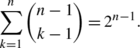
  • (c) Consider now all possible functions from S to M. The largest possible k is obviously k= cardS=n representing the cardinality mapping of S. From (b) we will then sum over 1≤k≤n giving

    

  • (d) An injection, card(S)=card(FS), from S to M where k≥n will mean the conditions  cardh _(i)=1, α≠β in S⇒Fα≠Fβ (where α and β represent any two id:s, not two in particular). This is easily seen to give $\binom{k}{n}$ possible functions as each mapping defines a subset in M with  card=n.

  From physics we recognize that the number of mappings in case b above, $\binom{n-1}{k-1}$ is equivalent to the number of states in Bose-Einstein statistics.

8.5 Collective Mappings Set to Sort

A novel feature of possible mappings to Sorts is that the image of an element could be an unspecified (fundamentally unspecified) member of some subsort/subcollection of S,h⊆S. The notion for such unspecified element is the blur of the elements in $h, \ \hat{U} h$. Given an element x in the domain (x∈M) we could assign the value $\hat{U} h$ to x. In contrast to mapping Sort → Set the ambiguity is now found in the codomain with id:s as members. Again the definition of collective functions Sort → Set will be the approach. It is important to point out when dealing with Sorts, care must be taken when something is defined that the definition will not be inconsistent with the basic axioms regarding id:s.

Definition 8.4

A Collective function F: M→S is characterized by

• (i) F(m ₁∪m ₂)=Fm ₁∪Fm ₂ where m ₁ and m ₂ are subsets of M.

• (ii) Fx ₁≠Fx ₂→x ₁≠x ₂ or as Fx _i in S, Fx ₁≠Fx ₂ means Fx ₁⊻Fx ₂. As before the cardinality of the image is less than or equal to the cardinality of the domain.

• (iii)  cardFm≤ cardm.

• (iv) The image of a subset m⊆M defines in general a subsort in S

  

  (7)

  with the usual meaning x∈m⇒Fx in h and for every α in h there is some y∈m such that Fy=α.

• (v) F can be specified by a partitioning of M into subsets M= ⋃^k m _i where for each m _i : Fm _i in S, FM=F[ ⋃^k m _i ]=h in S,  cardh=k. From this follows

  

  (8)

• vi Any permutation of the id:s in h leaves the collective function invariant.

8.6 Number of Distinct Functions Set to Sort

It was observed that the defining partitioning of the domain M= ⋃^k m _i is the only cause for distinction between two collective functions M→S. A partitioning of the set M is different from that of a Sort as we now have to have set-partitionings and not partitions of integers. As was seen each partition of M into k subsets will define an image of FM which defines a subsort of cardinality between 1 and k in S. Different subsorts will not give different functions if they have the same cardinality. Let us therefore determine the number of mappings for  cardFM=k defining subsort h _(k) in S. This must then equal the number of set-partitions of M into k subsets. This number is known as a Stirling number of the second kind denoted S(n,k) with a recursive formula S(n,k)=S(n−1,k−1)+kS(n−1,k), k≤n. This gives the number of onto functions from M→S. Next to get the number of into functions M→S is directly given from summing over all possible images each defined by  cardFM= cardh=i giving $\sum_{i=1}^{k} S(n, i)$. Finally to find the number of functions from a set M→S when  cardM=n we will sum over all functions from M _k →S from k=1 to k=n, where M _k denotes any set with cardinality k, which sum is given by the Bell number $B(n) = \sum_{k=1}^{n} S(n, i)$ recursivity given by $B(n + 1) = \sum_{i=0}^{n} \binom{n}{i} B(i)$.

8.7 Sort to Sort Functions

It is clear by now that the partitioning of the domain is crucial in the definition of collective functions S→T. Each partitioning H of S is then defined to be mapped into another Sort via a corresponding collective function F

where FH defines a subsort in the Sort T. As before  cardFh _(i)=1⇒  cardFH=k, for a partitioning into k subsorts of S,  cardS=n,  cardT=k. Each partitioning of S into k subsorts corresponds to the partitioning of the integer n into k sums corresponding to one onto function to T (any permutation in the codomain leaves the function invariant). The number of partitions of the integer n into k sums will therefore correspond to the number of onto functions to T. This number is denoted as p _k (n). The number of all into functions S _n →T _k is given by summation over k. For each p _i (n) we have $\sum_{i=1}^{k} p_{i}(n)$. All possible functions S→T,  cardT≥n is then given by $\sum_{i=1}^{n} p_{i}(n) = p(n)$ which has the estimate $p(n) = \frac{1}{4 \sqrt{3}} \mbox{exp} \ (\pi\sqrt{\frac{2n}{3}})$. The focus on the number of functions has been justified by the direct connection with statistics in physics, particularly quantum theory.

9 Functions as Operators from and to a Sort

In the context of Sorts there is a clear difference between functions defined as classes of ordered pairs and as operations. Collective functions being some analogue to class of pairs were associated to sets of cardinal numbers. A function regarded as an operation on an argument to give a certain value can “naively” be seen as an operation of “exchanging something for something else”, assuming we can give some meaning to functions as operations defined when Sorts are in question. If two such functions have values in some Sort, they can never be distinct, for in that case there must be some x in the domain for which fx⊥gx which cannot happen when the range is a Sort. As there is no way to select a particular value in the range R, it seems as the only possibility is to say that the value fx in R is completely undetermined, which is equivalent to saying $fx=\hat {U}R$ (the blur of R), whose value then can be seen as a “constant value” for f i.e. f a “constant function”.

9.1 Endomorphisms

A special class of functions from and to a Sort are endomorphisms. Considering endomorphisms of Sorts. where the argument and the value are in the same Sort, reveals some more possibilities for defining values of a function. The basic reason is that for fx=y, x and y in a Sort S, x and y can be related to each other in the common context of S. To take advantage of this we should try to create as much “structures” in S as possible. For instance, we have different subsorts in S, determined up to cardinality. As an illustration, let us look at possible values for an endomorphism (as an operator):

• (1) fx=x is a legal value as we have not changed anything, i.e. seeing f as an operator “exchanging something for something else”, fx=x represents “no exchange”. One can further impose the condition fx=x when x in h, h some subsort which accordingly is defined up to cardinality. This subsort then defines an invariant subsort relative f:s domain. Such an invariant subsort in f:s domain is then determined up to cardinality: fx=x when x in h,  cardh=n say.

• (2) Relating fx to some subsort h (if x in h does not involve a forbidden selection i.e. if we do not choose a particular value in h). Thus defining $fx=\hat{U}h$ is an allowed value when x in h. The reason why we can consistently demand that x is in h is that x already is in the context of h and can thus relate to id:s in h, meaning that x cannot be confused with some x′ not in h. We could also “assign” the value $\hat{U}Ch$, where Ch is the complement to h as x≠ all id:s in Ch. Continuing in similar ways to operators on two arguments fxy, one can define a limited number of different operators/functions. In this case one can create an analogue to binary operations. These operators can in turn be treated as new id:s forming Sorts of operators, etc. forming certain hierarchies of these.

10 Conclusion

In the second part of this paper I have been discussing consequences of introducing a weaker form of difference. This was called collective difference, characterized by lacking the normal individual difference when two objects are contrasted to each other, while being different in the sense of differently contributing to some common collective context, whole, collection etc. It was seen in the first part that the notion of order could be based on the basic notion of difference and similarity. To establish similarity between two things, reference to something third was seen as necessary. Therefore when regarding items with any collective difference this third item must be some collective common context expressed as: a is to C as b is to C, C representing some collective context. An example of this can be seen in the definition of a collective mapping F from a Sort: Fa=Fb where a and b are similar in relation to the common context of F which could be written as: a is to F as b is to F.

To form more mathematical structures working with Sorts, an important notion we have not been discussing at any length is operators, transformations etc. Due to non-ordinality such concepts will generate much poorer structures than in set theory, but might have aspects which are not naturally seen in a set-theoretical context. Certain classes of operators of Sorts representing endomorphisms could themselves be regarded as id:s, thus generating new Sorts. This procedure could then be repeated to yield hierarchies of Sorts, the structure of which might not easily be visible in a set-theoretic framework.

As a speculation, it is conceivable that not only particles could be indistinguishable in physics but also other aspects of a physical reality, such as physical states.

References

Bohm, D.: Quantum theory as an indication of a new order in physics part A: the development of new orders as shown through the history of physics. Found. Phys. 1(4), 359–371 (1971)
Bohm, D.: Quantum theory as a new order in physics, part B: implicate and explicate order in physical law. Found. Phys. 3(2), 139–155 (1973)
Bohm, D.: Some remarks on the notion of order, further remarks on order. In: Toward a Theoretical Biology, vol. 2, pp. 18–60 (1969)
Bohm, D.: Problems in the basic concepts of physics. In: Satyendranath Bose 70th Birthday Commemoration Volume, Part II, Calcutta, pp. 279–318 (1965). (an inaugural lecture delivered at Birkbeck College, February (1963))
Bohm, D.: Space, time and the quantum theory understood in terms of discrete process. In: Proc. of the Int. Conf. on Elementary Particles, Kyoto, Japan, pp. 252–286 (1965)
Hiley, B.J.: Process, distinction, groupoids and Clifford algebras: and alternative view of the quantum formalism. In: Coecke, B. (ed.) New Structures for Physics. Lecture Notes in Physics, vol. 813, pp. 705–750. Springer, Berlin (2011)
Bohm, D., Hiley, B.J.: The Undivided Universe. Routledge, London (1993)
Bohm, D.: Wholeness and the Implicate Order. Routledge and Kegan Paul, London (1980)
Ford, A.: Unpublished paper (2011)
Parker-Rhodes, A.F.: The Theory of Indistinguishables. Reidel, Dordrecht (1981)
Bohm, D., Peat, D.: Science, Order and Creativity. Bantam Books, New York (1987)
Open Access
This article is distributed under the terms of the Creative Commons Attribution License which permits any use, distribution, and reproduction in any medium, provided the original author(s) and the source are credited.
Author information
Authors and Affiliations
Corresponding author
Rights and permissions
Open Access This article is distributed under the terms of the Creative Commons Attribution 2.0 International License (https://creativecommons.org/licenses/by/2.0), which permits unrestricted use, distribution, and reproduction in any medium, provided the original work is properly cited.
About this article
Cite this article
Wikman, G. The Notion of Order in Mathematics and Physics. Similarity, Difference and Indistinguishability. Found Phys 43, 568–596 (2013). https://doi.org/10.1007/s10701-012-9688-y
Received:
Accepted:
Published:
Issue Date:
DOI: https://doi.org/10.1007/s10701-012-9688-y